Research on the Follow-Up Control Strategy of Biaxial Fatigue Test of Wind Turbine Blade Based on Electromagnetic Excitation

1  Introduction

To reduce the use of traditional fossil fuels and ensure sustainable energy development, there is an urgent need to develop renewable energy sources. Wind energy is regarded as one of the most promising renewable energy sources. However, since wind turbine blades are generally located in a complex working environment, the load of blades is larger in the actual operation, with a high change rate. The study shows that nearly 40% of blade failure is caused by fatigue damage. According to the latest detection standards for blade production, the blades must be carried out fatigue test [1]. At present, the mainstream methods of full-scale fatigue testing at home and abroad include forced displacement type and pendulum resonance type [2]. However, these two excitation methods are only suitable for loading in the vertical plane. When performing fatigue excitation test, only one axial surface of the blade can be loaded first, and the blade is rotated by 90 degrees. Then the other axial surface can be loaded. In fact, according to the test outline, a more accurate fatigue loading test should be the composite force in the biaxial direction of the blade. Under actual working conditions, the blade is subjected to a composite load in the two directions of flapwise and edgewise [3]. The biaxial electromagnetic excitation method is new compared to the traditional single-axis pendulum and other excitation methods. The biaxial electromagnetic excitation method can simultaneously carry out measurements loading in the flapwise and edgewise direction, which solves the above problems [4–7]. The effect produced by this composite loading method is more in line with the working conditions of the blade in actual service. Therefore, this dual-axis composite loading method is worth studying. However, in the fatigue test, the loading system is a high-order nonlinear time-varying system [8–10]. And it is difficult to ensure the real-time follow-up effect of the actual load and the target load during the fatigue loading process of the blade using traditional control methods. For example, the PID algorithm overshoots and responds slowly. Although the accuracy of RLS has improved, the magnitude of computation required is large; as a result, its response in high-frequency time-varying systems needs to be more sensitive.

The above traditional algorithm results in the system being unable to accurately apply the required load to the measured blade. This will affect the electromagnetic pulse excitation force applied to the blade, which in turn affects the steady-state amplitude of the blade. Finally, the fatigue test accuracy decreases, affecting the blade life prediction.

In terms of the following dynamic algorithm, several scholars at home and abroad have studied it. Ren et al. [11] used a terminal sliding mode controller to realize trajectory tracking control. Huang et al. [12] proposed a one-way fatigue following control strategy for blade sub-components based on LMS (Learning Management System) algorithm. Rigney et al. [13] used a combination of model predictive control and PI control to dynamically track known trajectories. Hou et al. [14] applied the control strategy of a single-neuron PID algorithm to intelligent vehicle trajectory tracking. Yasin et al. [15] designed an optimal dynamic following algorithm based on the penalty function. Chan et al. [16] used neural networks to realize steady-state tracking based on chiller stability problems. Zhang et al. [17] have applied fuzzy theory to the static loading test of wind turbine blades.

It has achieved corresponding control effects in its corresponding fields, but it is not suitable for the biaxial electromagnetic excitation test of wind turbine blades. For example, the research field of Ren et al. [11] and Hou et al. [14] is the trajectory recognition of intelligent vehicles. However, it is the field of trajectory tracking, focusing on non-high-frequency time-varying systems. For example, the following algorithm used by Rigney et al. [13], Chan et al. [16] is to predict its steady state. In this experiment, an adaptive tracking system needs to be developed to gradually reach the steady state of the experiment. Huang et al. [12] applied the LMS algorithm to the blade sub-component test, but its convergence speed was limited and was not suitable for the high-frequency scenario of this test. Zhang et al. [17] adopted a fuzzy control strategy in the static test, and the fuzzy control can better realize the adaptive change of output. Still, its static load scenario is to maintain the constant force, which is quite different from the time-varying system in this paper. However, the algorithm introduced by the above methodologist provides certain ideas for this paper in dynamic prediction and following effect, and this paper improves the idea of its following strategy to meet the needs of biaxial fatigue testing of electromagnetic excitation of wind turbine blades.

To solve the above problems, the FTRLS adaptive control algorithm of fuzzy forgetting factor is applied to the program design of the control system to realize the following load control. Since the forgetting factor in the FTRLS algorithm has a great influence on its convergence speed and accuracy, the larger the forgetting factor, the better its convergence speed and stability. But the tracking effect will become worse, and it is necessary to reduce the forgetting factor if you want to improve the tracking effect. To solve this contradiction, this paper uses fuzzy logic to control the forgetting factor in the FTRLS algorithm to achieve the adaptive change of the forgetting factor and it always maintains the optimal solution. Simulation and experimental results show that the algorithm can make the blade amplitude follow the set value, and the sampling accuracy is good, thereby shortening the test cycle.

2  Overview of the Design Scheme

The control system, actuator, and sensor constitute the wind turbine blade electromagnetic excitation fatigue loading equipment. The control system is composed of PC upper computer and electrical cabinet lower computer, and the upper computer is equipped with a human-computer interaction interface based on LabVIEW development. The actuator includes electromagnetic excitation equipment in two directions, flapwise and edgewise. The exciter in the flapwise and edgewise directions can operate simultaneously to achieve composite loading of the blades. And they can provide different excitation forces by controlling the magnitude and frequency of the current. The electromagnetic exciter is connected with the frequency conversion speed regulation system through the power cable and control cable, the load and other data are collected through the sensor, the feedback data of the sensor is transmitted to the control system, and the real-time tracking is realized by combining the adaptive algorithm. The main working parameters of the excitation system are adjusted through the frequency converter. The testing machine is shown in Fig. 1.

Figure 1: Design diagram of electromagnetic excitation fatigue testing machine

In this scenario, the wind turbine blades to be measured are fixed to the base by roots. A fixture is installed at the blade’s tip and connected to the exciter by a connecting mechanism. The electromagnetic pulse output beat of the exciter is controlled by the upper computer. And the fatigue test of different excitation forces is realized on the blades. At the same time, sensors are installed on the blades and in the output device to transmit the test data back to the host computer in real-time to realize the above series of control schemes.

3  Control System Design

3.1 Overview of Fast Transversal Recursive Least Squares (FTRLS) Adaptive Algorithm

An adaptive algorithm is an algorithm that automatically adjusts the processing method, order, parameters, boundaries, or constraints according to the data characteristics of the processed data to achieve the best processing effect. Traditional RLS has a small gradient estimation error and convergence speed, mainly because it can input both past and current signal vectors; this is shown in Fig. 2a. But too much calculation data at the same time leads to its large amount of operation. But because of this, the amount of data that needs to be processed at the same time will become larger, which will increase the amount of computation it needs at the same time. Its single iteration of the calculation magnitude is N2 (N represents the number of taps of the transverse filter, which is the storage space required to implement the filter), when the order N increases the corresponding amount of computation significantly increases, directly affecting the real-time response speed [18–20].

Figure 2: Algorithm flowchart of RLS and FTRLS, (a) Flow chart of RLS algorithm, (b) Flow chart of FTRLS algorithm

In view of the large computational amount of the RLS algorithm, many fast RLS algorithms have been proposed to overcome the contradiction between convergence speed and accuracy. Among them, the Fast Transversal Recursive Least Squares (FTRLS) algorithm is the most attractive and has been widely used. This paper combines the FTRLS algorithm with an electromagnetic excitation biaxial fatigue test. Finally, the dynamic quantities required for this experiment, such as input and output, are derived.

The FTRLS algorithm introduces forward prediction error and backward prediction error εb(k,n), which reduces the calculation amount of the iterative update formula and reduces the calculation amount to N [21], and the specific flow chart is shown in Fig. 2b.

As shown in Fig. 2b, the fast algorithm needs to solve both forward and backward linear prediction problems, which are completed by two predictors represented by and wb(k,n), and the predictors are composed of instantaneous posterior error ε(k,n) (using the filter coefficient of k to estimate the output at k), instantaneous a priori error e(k,n) (estimating the output of k-time using the filter coefficient of k-1) and least squares sum ξd(k,n). They exchange parameters with each other and finally make joint estimates. From the above process, the FTRLS is obtained.

Start with the forward prediction:

According to the biaxial fatigue test, the instantaneous input of k moment is x(k,n), and the performance parameter of k moment is A(k,n). Here the variable k is a time variable, and its unit is ‘s’. And the variable n is the output of the k moment, combined with the scenario used in this article, and its unit is ‘kN’.

The prior estimation error is:

ef(k,n)=AT(k−1,n)x(k,n)(1)

The posterior estimation error is:

εf(k,n)=γ(k−1,n)ef(k,n)(2)

The sum of the least squares is:

ξfmind(k,n)=λξfmind(k−1,n)+ef(k,n)εf(k,n)(3)

Because in practical use, new data is often more valuable than old data, a forgetting factor λ is less than or equal to 1 is introduced in Eq. (3), making the weight of old data smaller and smaller. However, referencing old data can increase the stability of algorithm operation, so the weight occupied by old data needs to be adjusted in real-time according to the actual situation, and it needs to be achieved by real-time changes in the forgetting factor λ, which will be studied in the next chapter.

where conversion factor

γ(k,n+1)=λξfmind(k−1,n)ξfmind(k,n)γ(k−1,n)(4)

where gain vector

ϕ(k,n+1)=[0ϕ(k−1,n)]+ef(k,n)λξfmind(k−1,n)A(k,n)(5)

where performance parameter

A(k,n)=[1−wf(k−1,n)](6)

Then the final forward prediction coefficient vector wf(k,n) is:

wf(k,n)=wf(k−1,n)+ϕ(k−1,n)εf(k,n)(7)

Then make a backward prediction:

The prior estimation error is:

eb(k,n)=λξbmind(k−1,n)ϕ(k,n)(8)

The posterior estimation error is:

εb(k,n)=γ(k,n)ef(k,n)(9)

The sum of the least squares is:

ξbmind(k,n)=λξbmind(k−1,n)+eb(k,n)εb(k,n)(10)

The updated equation for ϕ(k,n) is:

[ϕ(k,n)0]=ϕ(k,n+1)−eb(k,n)λξbminb(k−1,n)[−wb(k−1,n)1](11)

The backward prediction coefficient vector update equation is:

wb(k,n)=wb(k−1,n)+ϕ(k,n)εb(k,n)(12)

Then the joint process estimation is carried out: The parameters are set according to the biaxial fatigue test: d(k) is the desired load signal and x(k,n) is the actual input load signal.

The a priori error between the input signal and the desired signal can be expressed as:

e(k,n)=d(k)−wT(k−1,n)x(k,n)(13)

The relationship between the a priori error and the a posteriori error is:

ε(k,n)=e(k,n)γ(k,n)(14)

The relationship between the a priori error and the a posteriori error is:

w(k,n)=w(k−1,n)+ϕ(k,n)ε(k,n)(15)

Therefore, the final FTRLS-based adaptive weight control strategy is shown below:

{y(k,n)=wT(k−1,n)x(k,n)e(k,n)=d(k,n)−y(k,n)w(k,n)=w(k−1,n)+ϕ(k,n)ε(k,n)(16)

In Eq. (16): y(k,n) is the system output; x(k,n) is the system input; e(k,n) is the system estimation error; ϕ(k,n) is the gain vector at time k; w(k,n) is the weight vector at time k, d(k,n) is a reference signal, and the following uses y(k), x(k), ϕ(k), e(k), w(k), d(k) to simplify the description.

Among them, the weight vector w(k) plays a major role in the convergence speed and accuracy of the algorithm, and the weight vector is mainly affected by the forgetting factor λ in ϕ(k).

3.2 Fuzzy Forgetting Factor FTRLS Algorithm

Fuzzy logic consists of four steps, namely: (1) Fuzzy sets of design parameters; (2) Design fuzzy rules; (3) Design fuzzy operators; (4) Defuzzing [22–25]. The fuzzy control logic used in this paper uses two inputs, i.e., the residual and residual change rate of the controlled dynamics, and one output, the forgetting factor.

The purpose of using the forgetting factor in the FTRLS algorithm is to guarantee that the impact of previous data on the present is as low as possible. So that in an unsteady state environment, the filter can still work, and has a strong dynamic tracking capability. At the same time, fuzzy logic is used in this article to adjust the forgetting factor of the control signal in real time instead of using a fixed forgetting factor.

3.2.1 Fuzzy Sets of Design Parameters

The absolute value of the residual E(k) reflects the gap between the measured system dynamic value and the identification model value. In the identification process, the larger the absolute value of E(k), the larger the gap between the measured system dynamic value and the identification model value; in this case, to guarantee that the algorithm identification results quickly converge to the actual dynamic value, the value of the forgetting factor λ should be reduced, on the contrary, the absolute value of the residual E(k) becomes smaller, the forgetting factor λ strain is large, so as to enhance the robustness of the system.

In order to avoid the error caused by the system response being too sensitive to a single measurement result, we use the residual average of the shorter time series as the evaluation function V(k) to identify the degree of compatibility between the identification value and the dynamic value of the system, then select ΔV(k) that can reflect the changing trend of the evaluation function. Finally, using V(k) and ΔV(k) as the input variables of the system, the expressions of the two inputs at k time are shown in Eqs. (17) and (18).

V(k)=1L∑i=k−Lk|E(i)|(17)

ΔV(k)=1t[V(k)−V(k−t)](18)

Therefore, the fuzzy input used in this control strategy is the average value of the residual time series V and the residual change rate ΔV, and then stably identifies the dynamic loading time-varying model. The block diagram of the algorithm based on fuzzy logic is shown in Fig. 3, where y(k) is the actual output, x(k) is the actual input, E(k) is the residual, and d(k) is the ideal input. The controlled object is the target load to be output to the blade.

Figure 3: Block diagram of the fuzzy-FRLS algorithm

3.2.2 Design Fuzzy Rules and Fuzzy Operators

The specific idea is: ① Determine the input and output and its fuzzy set, ② Define the input and output membership function, and ③ Establish fuzzy control rules through the fuzzy control table.

Firstly, the V, ΔV, λ signals are blurred, and the fuzzy sets of V and ΔV are determined to be {NE, ZO, PE} (NE is negative, ZO is zero, PE is positive), and the fuzzy domain of the forgetting factor is {NB, NS, ZO, PS, PB} (NB is negative big, NS is negative small, ZO is zero, PS is positive small, PB is positive big). Then select the trigonometric function as the membership function of the controller, as shown in Fig. 4.

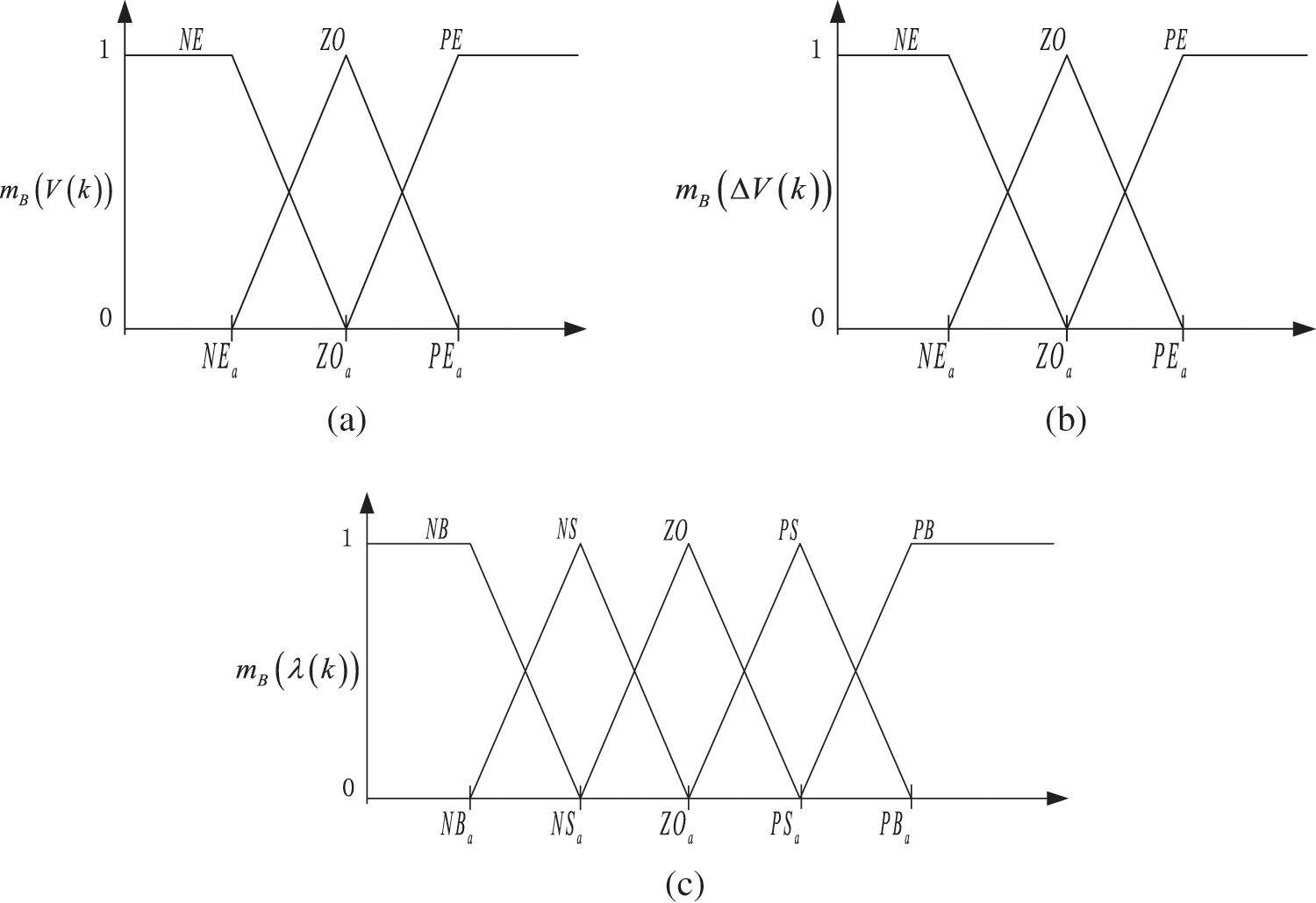
Figure 4: Distribution range of each member function, (a) Residual mean V, (b) Residual rate of change ΔV, (c) Variable forgetting factor λ

When both V and ΔV are PE, the identification result and the actual result deviate greatly and the deviation increase gradually, and the forgetting factor λ should be NB to ensure that the identification result converges quickly near the actual result. When V is PE and ΔV is NE, it means that the deviation between the identification result and the actual result is large, but the gap is gradually narrowing, and the forgetting factor λ is NS. When both V and ΔV are NE, it means that the deviation between the identification result and the actual result is small, the deviation is gradually narrowing, and the forgetting factor λ should be PB to suppress the influence of noise disturbance on the recognition accuracy of system parameters. Correspondingly, when V is NE, ΔV is PE, the forgetting factor λ should be PS.

Guided by the above knowledge, fuzzy control rules are established, as shown in Fig. 5.

Figure 5: Fuzzy control rules

3.2.3 The Defuzzification Adopts the Center of Gravity Method

The output is shown in the following equation:

λ[k]=∑i=1qλi[k]mB(λi[k])∑i=1qmB(λi[k])(19)

where q is the approximate number of member functions, and mB(x) represents the value of the member function at the x position.

3.3 Fuzzy Logic-Based Filtering and Amplitude Control Policy

The inputs and weights of the system loading are shown in Eqs. (20)–(23), respectively, where x(k) is the system input at moment k, y(k) is the system output at moment k, and w(k) is the vector of weights at moment k.

Flapwise direction input:

x1(k)=[x1(k),x1(k−t)]T=[A1sin⁡(ω1k),A1cos⁡(ω1k)]T(20)

w1(k)=[w2,w3](21)

Edgewise direction input:

x2(k)=[x2(k),x2(k−t)]T=[A2sin⁡(ω2k),A2cos⁡(ω2k)]T(22)

w4(k)=[w5,w6](23)

Substituting Eqs. (20)–(23) into Eq. (16), respectively, the final output function of the system is:

y1(k)=w2A1sin⁡(ω1k)+w3A1cos⁡(ω1k)=A1w22+w32[w2⋅sin⁡(ω1k)w22+w32+w3⋅cos⁡(ω1k)w22+w32](24)

y2(k)=w5A2sin⁡(ω2k)+w6A2cos⁡(ω2k)=A2w52+w62[w5⋅sin⁡(ω2k)w52+w62+w6⋅cos⁡(ω2k)w52+w62](25)

Let cos⁡φ1=w2w22+w32, sin⁡φ1=w3w22+w32, Ay1=A1w22+w32, cos⁡φ2=w5w52+w62, sin⁡φ2=w6w52+w62, Ay2=A2w52+w62 and substitute them into Eqs. (24) and (25) to obtain the simplified system output as shown in Eqs. (26) and (27), respectively.

y1(k)=Ay1sin⁡(ω1k+φ1)(26)

y2(k)=Ay2sin⁡(ω2k+φ2)(27)

From Eqs. (26) and (27), it can be seen that the system output can be compensated by adjusting w2, w3, w5 and w6 in the weight vector w1(k) and w4(k). The weight vector w is mainly affected by the forgetting factor λ, and the forgetting factor will be obtained in real-time through the fuzzy controller, and finally the optimal weight at k time is selected, so as to realize the real-time follow-up of the actual load to the expected load.

4  Simulation Analysis

In MATLAB/Simulink, a simulation model of the testing machine is constructed to verify the effectiveness of the control strategy. Firstly, taking the flapwise direction as an example, the load and amplitude response of blades under the traditional RLS and fuzzy FTRLS algorithms are explored. The simulation results are presented in Fig. 6.

Figure 6: Load and amplitude response under traditional RLS algorithm

Fig. 6 shows the load and steady-state response curves of the system when the blades are excited by electromagnetic pulses, and the four curves are the results of the target response and traditional RLS simulation. It can be seen that the traditional RLS algorithm has a very serious hysteresis effect and overshoot problem for the following of the pulse signal of the step, and the peak can only be reached after 0.15 s, and the overshoot is −9%, which leads to amplitude attenuation and phase hysteresis of the amplitude, and a large steady-state error with the target.

The simulation results after using the fuzzy FTRLS algorithm to control the strategy are shown in Fig. 7. The problems of hysteresis and overshoot are significantly improved, and the actual load can stably follow the expected load, which achieves the expected following effect.

Figure 7: Load and amplitude response under fuzzy FTRLS algorithm

Next, the biaxial fatigue simulation is carried out [26], and its parameters are determined according to the field test of biaxial electromagnetic fatigue loading, and the sinusoidal excitation force is input in the flapwise and edgewise direction, and the amplitude of the flapwise direction is between ±0.15 m, and the frequency is 1.0 Hz. The edgewise direction amplitude is between ±0.08 m, and the frequency is 1.5 Hz. Based on the above model, the dual-axis following effect is shownin Fig. 8.

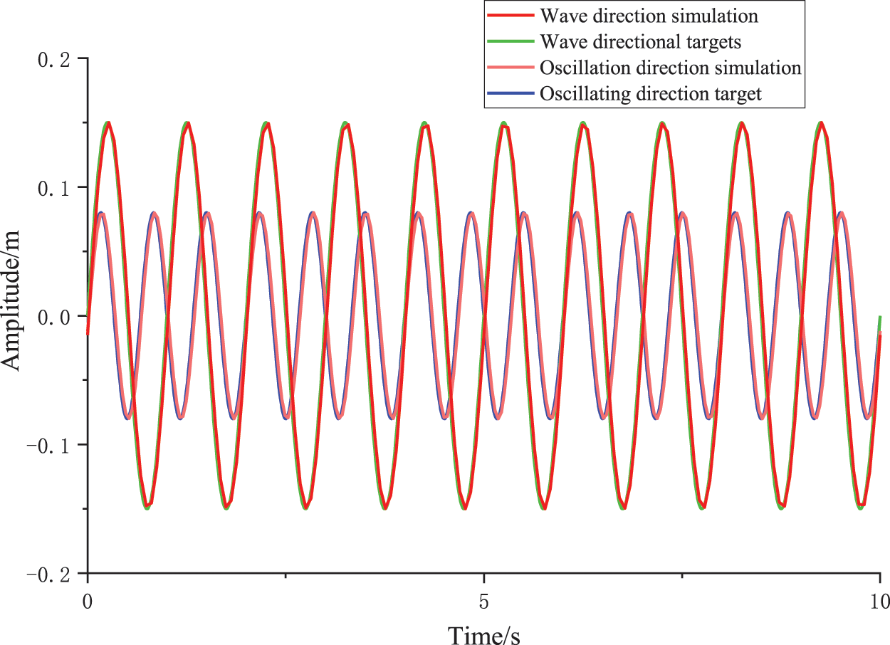
Figure 8: Biaxial fatigue following effect under fuzzy FTRLS control strategy

As shown in Fig. 8, in the whole process, except for a small range of amplitude attenuation at the peak, the overall following effect meets the requirements of the algorithm design. However, the simulation is ideal, so field tests are required for further verification.

5  Test and Analysis

Through the above design, a blade electromagnetic fatigue test platform was built in this unit, and the sinusoidal force of biaxial loading was analyzed according to the test requirements, and the following effect of the blade and the loading source was analyzed, and the test parameters were shown in Table 1.

The whole test loading system includes the blade, electromagnetic fatigue, test base, upper computer, control cabinet, sensor, etc. The test system is shown in Fig. 9.

Figure 9: Field trial

The experimental subject is a two-m-long model of wind turbine blades. This blade is made with the same process as the actual large blade now in service. The main beam and web body are made of glass fiber composite, the web and core are sandwich structures, and the middle sandwich layer uses PVC foam board. This model uses the same structure and materials as the current mainstream large service blades, which ensures the reliability of this test result.

The blade model is fixed on the test base through the root, the electromagnetic excitation device in the biaxial direction is fixed close to the tip of the blade, and the blade output suitable excitation force is fatigue loaded through the iron core, connecting rod, etc.

Taking the flapwise direction as an example, the actual load and amplitude following response when using different algorithm control strategies are collected by the strain acquisition system in the actual experiment, and the results are presented in Fig. 10.

Figure 10: Load and amplitude response using traditional RLS algorithm

In the case of using the traditional RLS algorithm, the acquisition curve of the strain acquisition system is shown in Fig. 10. The actual load response and the target impulse response do have certain lag and overshoot problems, resulting in the blade fatigue curve cannot form simple harmonic vibration and cannot achieve the steady-state response, so the experimental data using this algorithm cannot accurately calculate the strain. In the actual test, the blade cannot achieve resonance in this state, which will cause serious damage to the blade itself and mislead the calculation of the fatigue life of the blade.

Fig. 11 shows the fatigue test response following the introduction of the fuzzy FTRLS algorithm. It can be seen from the figure that the actual load is basically the ideal pulse load, and the blade has a stable accumulation process in the initial stage and finally enters the steady state when the excitation force and the vibration energy consumption of the blade are equal. The actual test blade finally achieves the resonance effect, which verifies the feasibility of the algorithm.

Figure 11: Load and amplitude response using fuzzy FTRLS algorithm

Next, the blade is subjected to biaxial fatigue loading because the hetero frequency loading is more practical than the same frequency. The experimental parameters are the flapwise frequency is 1 Hz, and the edgewise frequency is 1.5 Hz. Under the excitation of the two axes’ respective frequencies, the flapwise and edgewise direction fatigue test curve is shown in Fig. 12.

Figure 12: Biaxial fatigue loading test results, (a) Flapwise direction amplitude. (b) Flapwise direction amplitude error. (c) Edgewise direction amplitude. (d) Edgewise direction amplitude error

As shown in Fig. 12a, the direction of flapwise has a following effect at the beginning, and a stable resonance is reached in 10 s. As can be seen from Fig. 12c, the edgewise direction begins to follow in about 0.5 s and reaches resonance in about 7 s.

It can be seen from Fig. 12 that whether it is oscillating or flapwise direction when using the traditional RLS algorithm, the strain curves in both directions are difficult to maintain stability, and the phenomenon of overshoot between the actual strain curve and the target strain frequently occurs. Combined with the fuzzy FTRLS algorithm, the key point strain of the blade flapwise and edgewise direction can reach a stable and recommended value, indicating that the control system can accurately control the strain in real time so that it can continue to approach the recommended value and finally reach steady state.

This is shown in Figs. 12b and 12d, and it can be seen from the error curve that after the fuzzy FTRLS algorithm is adopted, the bidirectional loading error is controlled within 4%, which achieves the expected following effect. Therefore, the effectiveness of the design scheme and the following algorithm is fully verified.

6  Conclusion

Based on the biaxial fatigue test of the electromagnetic force of wind turbine blades, this paper first designs a set of control schemes from the computer to the adaptive controller to the actuator and then develops an FTRLS algorithm based on fuzzy forgetting factor for the real-time tracking of dynamic quantities in the experiment, and finally builds a test platform to verify the feasibility of the algorithm, and concludes the following:

1) Through the analysis of the electromagnetic force biaxial fatigue test data, it is found that the biaxial fatigue test system for the electromagnetic force of wind turbine blades requires a high frequency of loads and rapid changes. The traditional RLS algorithm conflicts between convergence speed and accuracy, and it is necessary to develop a control strategy with fast response speed and strong robustness to meet the needs of the biaxial fatigue test.

2) In this paper, an FTRLS control strategy based on the fuzzy forgetting factor is adopted, and the field test data show that the dynamic tracking error of flapwise and edgewise direction is controlled within 4%, which meets the test requirements. Therefore, this control strategy can better control the controlled object and realize the real-time follow-up of its dynamic quantity. At the same time, this control strategy also provides valuable experience for electromagnetic excitation biaxial fatigue testing.

Acknowledgement: The authors would like to acknowledge the Institute of Wind Power Blade New Technology Industrialization of Shandong University of Technology for providing technical guidance for this project.

Funding Statement: This research was funded by the National Natural Science Foundation of China (Grant Number 52075305).

Author Contributions: The authors confirm contribution to the paper as follows: study conception and design: Leian Zhang, Wenzhe Guo; data collection: Weisheng Liu; analysis and interpretation of results: Chao Lv, Jiabin Tian; draft manuscript preparation: Wenzhe Guo. All authors reviewed the results and approved the final version of the manuscript.

Availability of Data and Materials: The data used in this research are available upon the request from the corresponding author. Some data is not available because of the confidentiality of the industry.

Conflicts of Interest: The authors declare that they have no conflicts of interest to report regarding the present study.

References

1. Zhang, L., Guo, Y., Wang, J., Huang, X., Wei, X. et al. (2019). Structural failure test of a 52.5 m wind turbine blade under combined loading. Engineering Failure Analysis, 103(11), 286–293. [Google Scholar]

2. Zhang, M., Tan, B., Xu, J. (2018). Smart fatigue load control on the large-scale wind turbine blades using different sensing signals. Renewable Energy, 87(4), 111–119. [Google Scholar]

3. Liao, G., Wu, J., Zhang, H. (2019). Wind turbine blades biaxial inertia vibration fatigue loading system and control. Acta Energiae Solaris Sinica, 40(2), 356–362. [Google Scholar]

4. Eder, M. A., Belloni, F., Tesauro, A., Hanis, T. (2017). A multi-frequency fatigue testing method for wind turbine rotor blades. Journal of Sound and Vibration, 388(2), 123–140. [Google Scholar]

5. White, D., Desmond, M., Gowharji, W., Beckwith, J. A., Meierjurgen, K. J. (2011). Development of a dual-axis phase-locked resonant excitation test method for fatigue testing of wind turbine blades. ASME International Mechanical Engineering Congress & Exposition, 54907, 1163–1172. [Google Scholar]

6. Lu, L., Zhu, M., Wu, H., Wu, J. (2022). A review and case analysis on biaxial synchronous loading technology and fast moment-matching methods for fatigue tests of wind turbine blades. Energies, 15(13), 4881. [Google Scholar]

7. Zhang, L., Yu, X., Wei, X., Liu, W. (2018). Joint excitation synchronization characteristics of fatigue test for offshore wind turbine blade. AIP Advances, 19(1), 5512–5525. [Google Scholar]

8. Li, D. (2023). Wind turbine blades load matching method under biaxial fatigue test. Journal of Engineering Mechanics and Machinery, 8(1), 1–11. [Google Scholar]

9. Wang, X., Li, W., Liu, Y., Wen, Z. (2021). Constant tension control of umbilical cable tension-bending combined fatigue testing machine. Journal of Harbin Engineering University, 42(5), 632–640. [Google Scholar]

10. Dreidy, M., Mokhlis, H., Mekhilef, S. (2017). Inertia response and frequency control techniques for renewable energy sources: A review. Renewable & Sustainable Energy Reviews, 69, 144–155. [Google Scholar]

11. Ren, D., Zhang, J., Zhang, J., Cui, S. (2011). Trajectory planning and yaw rate tracking control for lane changing of intelligent vehicle on curved road. Control and Dynamics, 54(3), 630–642. [Google Scholar]

12. Hang, X., Tao, L., Yao, J., Zhang, L., Wei, X. (2017). Research on following control strategy of wind turbine blade bolt sleeve fatigue testing machine. Journal of Solar Energy, 38(8), 2106–2111. [Google Scholar]

13. Rigney, B., Pao, L., Lawrence, D. (2009). Nonminimum phase dynamic inversion for settle time applications. IEEE Transactions on Control Systems Technology, 17(5), 989–1005. [Google Scholar]

14. Hou, Y., Zhu, Z. H. (2015). Application of single-neuron PID control algorithm in intelligent vehicle control system. Control and Instruments in Chemical Industry, 42(2), 134–138. [Google Scholar]

15. Yasin M., Hussain M. J. (2016). A novel adaptive algorithm addresses potential problems of blind algorithm. International Journal of Antennas and Propagation, 5, 1–8. [Google Scholar]

16. Chan, T., Chang, Y., Huang, J. (2017). Application of artificial neural network and genetic algorithm to the optimization of load distribution for a multiple-type-chiller plant. Building Simulation, 10(2), 711–722. [Google Scholar]

17. Zhang, L., Huang, X., Yuan, G. (2015). Control algorithm of static loading test for wind turbine blade based on fuzzy theory. International Journal of Smart Home, 9(4), 107–116. [Google Scholar]

18. Paleologu, C., Benesty, J., Ciochina, S. (2008). A robust variable forgetting factor recursive least-squares algorithm for system identification. IEEE Signal Processing Letters, 15, 597–600. [Google Scholar]

19. Elisei-Iliescu, C., Dogariu, L. M., Paleologu, C., Benesty, J., Enescu, A. A. et al. (2020). A recursive least-squares algorithm for the identification of trilinear forms. IEEE Transactions on Signal Processing, 13(6), 135. [Google Scholar]

20. Zhang, R., Zhao, H. (2021). A novel method for online extraction of small-angle scattering pulse signals from particles based on variable forgetting factor RLS algorithm. Sensors, 21(17), 5759. [Google Scholar] [PubMed]

21. Wan, C., Chen, D., Yang, J. (2022). Pulse rate estimation from forehead photoplethysmograph signal using RLS adaptive filtering with dynamical reference signal. Biomedical Signal Processing and Control, 71(B), 1746–8094. [Google Scholar]

22. Liang, H., Zou, J., Zuo, K., Muhammad, J. K. (2020). An improved genetic algorithm optimization fuzzy controller applied to the wellhead back pressure control system. Mechanical Systems and Signal Processing, 142, 888–3270. [Google Scholar]

23. Precup, R. M., David, R. C., Petriu, E. M. (2016). Grey wolf optimizer algorithm-based tuning of fuzzy control systems with reduced parametric sensitivity. IEEE Transactions on Industrial Electronics, 64(1), 527–534. [Google Scholar]

24. Zakharov, Y. V., Nascimento, V. H. (2013). Dcd-RLS adaptive filters with penalties for sparse identification. IEEE Transactions on Signal Processing, 61(12), 3198–3213. [Google Scholar]

25. Pan, Y., Wu, Y., Hak-Keung, L. (2022). Security-based fuzzy control for nonlinear networked control systems with dos attacks via a resilient event-triggered scheme. IEEE Transactions on Fuzzy Systems, 30(10), 4359–4368. [Google Scholar]

26. Huang, X., Zhang, L., Yuan, G., Wang, N. (2015). Coupling mechanism of dual-excitation fatigue loading system of wind turbine blades. Journal of Vibroengineering, 17(5), 2624–2632. [Google Scholar]