
 Submit a Paper
 Propose a Special lssue
 Open Access
ARTICLE

Diagnosis of Disc Space Variation Fault Degree of Transformer Winding Based on K-Nearest Neighbor Algorithm
1 Department of Power and Electrical Engineering, Northwest A&F University, Yangling, 712100, China
2 NARI Group, Beijing Kedong Electric Power Control System Co., Ltd., Beijing, 100000, China
3 Huangling Mining Group Co., Ltd., Shanxi Coal and Chemical Industry Group, Huangling, 716000, China
* Corresponding Author: Song Wang. Email:
(This article belongs to the Special Issue: Advances in Modern Electric Power and Energy Systems)
Energy Engineering 2023, 120(10), 2273-2285. https://doi.org/10.32604/ee.2023.030107
Received 22 March 2023; Accepted 01 June 2023; Issue published 28 September 2023
 View Full Text
 Download PDF
Abstract
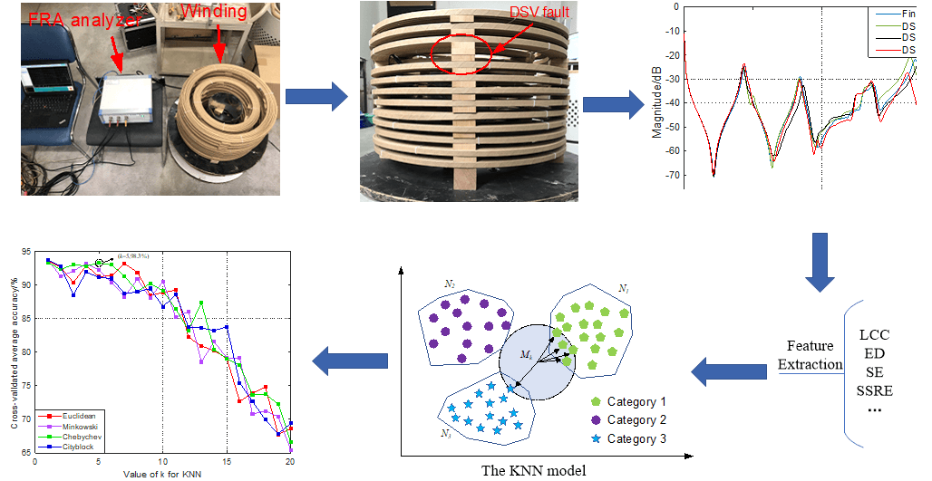
Winding is one of the most important components in power transformers. Ensuring the health state of the winding is of great importance to the stable operation of the power system. To efficiently and accurately diagnose the disc space variation (DSV) fault degree of transformer winding, this paper presents a diagnostic method of winding fault based on the K-Nearest Neighbor (KNN) algorithm and the frequency response analysis (FRA) method. First, a laboratory winding model is used, and DSV faults with four different degrees are achieved by changing disc space of the discs in the winding. Then, a series of FRA tests are conducted to obtain the FRA results and set up the FRA dataset. Second, ten different numerical indices are utilized to obtain features of FRA curves of faulted winding. Third, the 10-fold cross-validation method is employed to determine the optimal k-value of KNN. In addition, to improve the accuracy of the KNN model, a comparative analysis is made between the accuracy of the KNN algorithm and k-value under four distance functions. After getting the most appropriate distance metric and k-value, the fault classification model based on the KNN and FRA is constructed and it is used to classify the degrees of DSV faults. The identification accuracy rate of the proposed model is up to 98.30%. Finally, the performance of the model is presented by comparing with the support vector machine (SVM), SVM optimized by the particle swarm optimization (PSO-SVM) method, and random forest (RF). The results show that the diagnosis accuracy of the proposed model is the highest and the model can be used to accurately diagnose the DSV fault degrees of the winding.Graphic Abstract
Keywords
Power transformers play an important role in voltage transformation and energy transmission for power systems [1,2]. As the essential equipment within the power station and substation, the reliable operation of power transformers is of great importance for the safe and stable operation of the energy internet. A research report on the failure data of transformers shows that winding deformation has been one of the main causes of transformer failures [3]. Because the transformer winding is slightly deformed and difficult to detect in the early stage of a failure, minor failure accumulates over a long period of time, while the winding insulation ages and the ability to resist short circuit decreases [4]. Once the transformer winding is impacted by the short circuit current, its powerful electro-dynamic poles may cause serious damage to the transformer. Therefore, accurate fault prognostic is essential for preventing slight winding deformation developing into catastrophic accidents and ensuring the healthy operation of the power system.
To accurately detect winding deformation, lots of detection methods have been developed, such as the short circuit impedance method [5], the low voltage pulse method [6], and the frequency response analysis (FRA) method [7–9]. Among these diagnostic methods, the FRA method has emerged as a very powerful and effective off-line detection tool due to its simple operation, good stability, and high sensitivity. The FRA method relies on the interpretation of the deviation between the reference FRA curve and the subsequently measured one. To date, several approaches have been proposed to extract the features of FRA curves and assess the fault of the transformer winding, such as transformer winding modeling [10], statistical index method [11], and transfer function method [12]. However, due to the indispensability of expertise knowledge and complexity of the FRA results, it is still difficult to identify and diagnose the fault type, fault location, and fault degree of the windings based on the above analysis methods.
With the rapid growth of artificial intelligence, machine learning (ML) algorithms have been widely and successfully used in the FRA field to identify the faults of winding. By using ML algorithms, the diagnosis and interpretation results based on FRA curves are made accurately and automatically without relying too much on expert experience. Therefore, some misdiagnoses can be effectively avoided. In reference [13], a support vector machine (SVM) is employed to identify fault types and degrees. In reference [14], a SVM model is used to locate and quantify the radial buckling fault. Mao et al. [15] use SVMs to accurately identify the winding type. In reference [16], Luo applies the artificial neural network (ANN) to recognize the extents of the deformation of winding by using some statistical indicators. In addition, the hierarchical clustering method has also been successfully introduced to explore the winding fault types [17].
As a supervised method, the K-Nearest Neighbor (KNN) algorithm has the advantages of high accuracy, insensitivity to noise, and low complexity. It has been used to address classification and regression. Especially, since KNN is only concerned with a small number of adjacent samples when making classification decisions and it does not rely on the method of discriminating the category to which it belongs, it has a good classification effect for different sample sets that cross or overlap more. However, until now, the application of KNN based on FRA for the identification of the typical winding fault degrees is rare. Therefore, in this paper, a diagnosis model combining the FRA method and KNN is proposed to identify the disc space variation (DSV) fault degrees of the transformer winding. First, plenty of FRA tests are conducted on a winding model with four different degrees of DSV fault to acquire the FRA dataset. Second, several different numerical indices are selected to extract the characteristics of the FRA curves caused by DSV faults. Third, the 10-fold cross-validation method is employed to determine the optimal k-value of KNN. To realize the optimal performance of the KNN model for fault classification, the relationship between the accuracy of the KNN model and the k-value is compared under different distance functions. Then, the KNN model is established by using the selected k-value and the best distance function to identify the DSV fault degrees of the transformer winding. Finally, the diagnostic performance of the proposed model, including accuracy rate and running time, is compared with that of traditional SVM, SVM optimized by the particle swarm optimization (PSO-SVM), and the random forest (RF).
The rest of this paper is structured as follows. Section 2 is the principle of the FRA test and DSV fault settings. The features existing in the deviation of the FRA curves caused by faults are extracted by using numerical indices described in Section 3. Section 4 is the diagnosis of DSV fault degrees by KNN. The application procedure of the proposed model, results analysis, and comparison with SVM, PSO-SVM, and RF are all shown in this section. Section 5 is the conclusion.
2 Principle of FRA and DSV Fault of Winding
2.1 Fundamentals of the FRA Method
FRA is a non-destructive detection method that is capable of detecting mechanical deformation of the core and winding. The diagram of FRA tests is shown in Fig. 1. In the FRA method, the low-voltage sweep frequency excitation signals are injected into one terminal of a winding, and corresponding response signals are measured from the other terminal of the winding. Then, by calculating the amplitude of the ratio of response voltage to the input voltage, the amplitude of the frequency response can be obtained, as described in Eq. (1). Finally, the FRA curve can be got by plotting the amplitude of the frequency response with respect to frequencies. Since the winding can be equivalent to a passive linear two-port network consisting of resistance, inductance, mutual inductance, conductance, and capacitance, any change of the geometry of the winding caused by fault will lead to the change of the FRA curve. Then, by analyzing and interpreting the deviation of the current FRA curve and initial FRA curve, the state of the winding will be diagnosed.
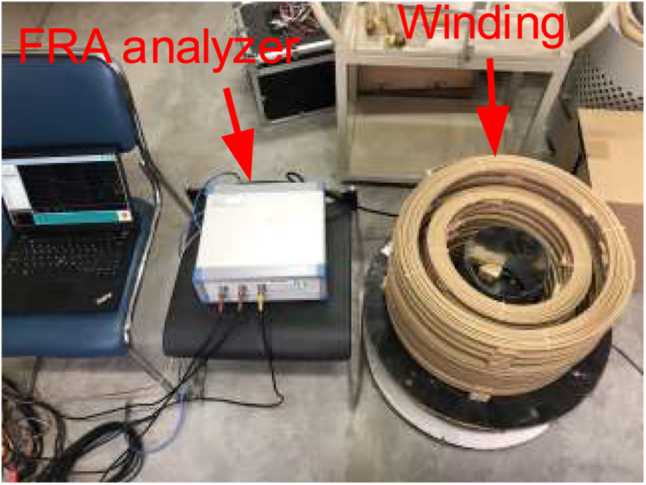
Figure 1: Diagram of FRA tests
where,
In IEEE [18] and IEC [19] standards, four typical FRA test connection ways are introduced. They are end-to-end voltage ratio (EE), end-to-end short-circuit (EES), capacitive inter-winding (CIW), and inductive inter-winding connections (IIW), as shown in Fig. 2. In Fig. 2a, the sweep frequency signals are injected into one terminal of a winding while the response signals are received from the other terminal. At the same time, the secondary winding of the same phase is left open during the test. Because this way can obtain the frequency response of each winding separately, so it is the most widely used connection. In this paper, the EE connection is used.
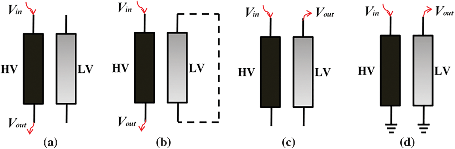
Figure 2: FRA test configurations. (a) EE, (b) EES, (c) CIW, and (d) IIW
The laboratory winding with the type of continuous discs is shown in Fig. 3. The height of the winding is 230 mm and the winding has 12 discs. The inner and outer diameters of a disc are 370 and 530 mm, respectively. There are four different DSV fault degrees in this study. By altering the height of the spacer between adjacent discs, the DSV faults with different levels are achieved, namely ∆h, 2∆h, 3∆h and 4∆h, as shown in Fig. 3. ∆h is 10 mm. It needs to state that the DSV faults with different degrees that occurred in different locations of the winding are all taken into consideration to acquire more FRA results.
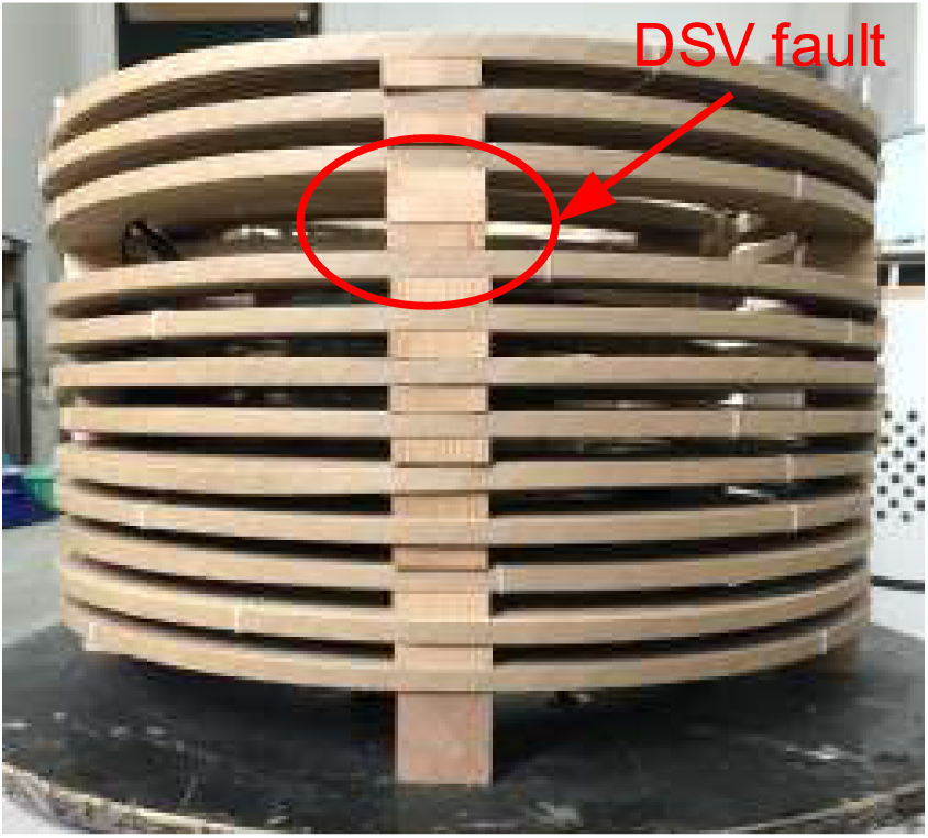
Figure 3: Winding with a DSV fault
The measured FRA curves with four different DSV fault degrees at different locations of the winding are shown in Fig. 4. It needs to state that since the number of FRA curves is very large, only a part of them are shown in Fig. 4.
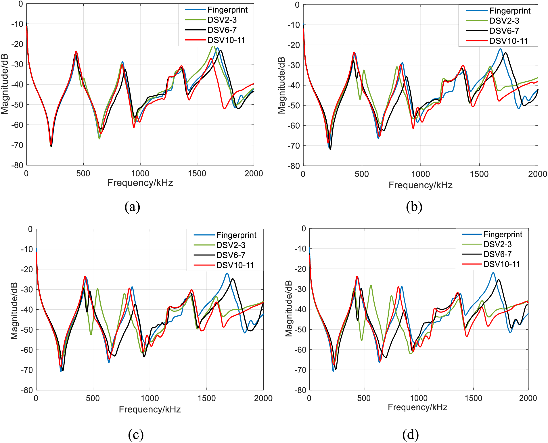
Figure 4: The FRA curves under different DSV fault degrees. (a) Fault degree 1; (b) Fault degree 2; (c) Fault degree 3; (d) Fault degree 4
3 Feature Extraction of FRA results
3.1 Selection of Numerical Indices
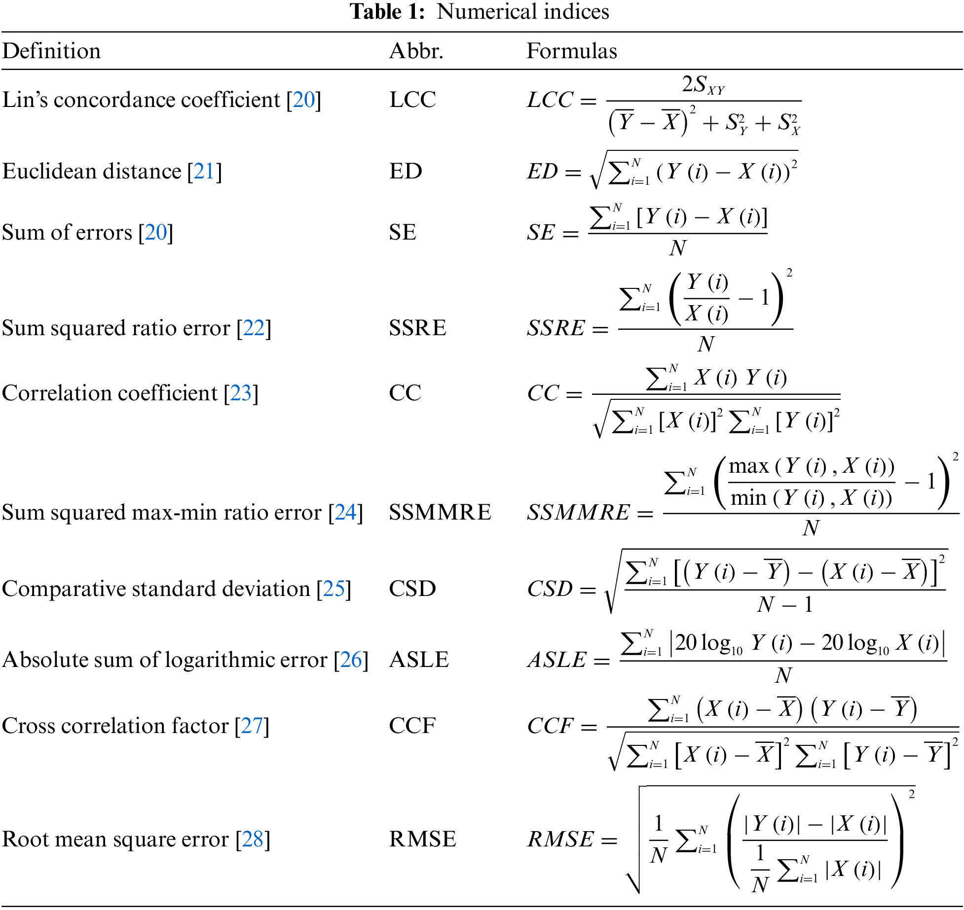
To accurately classify the DSV fault degrees of the winding, the features existing in the deviation of the FRA fingerprint and current FRA curves should be precisely obtained. In this study, according to the contributions of references [20–28], ten different types of numerical indices are selected, as shown in Table 1. All of the indices in Table 1 are calculated based on the magnitude vectors.
To eliminate the influence of the dimension of different numerical indices, the Min-Max method is used to normalize the indices. The normalization equation is expressed as:
where, x represents the feature variable that needs to be normalized.
4 Diagnosis of DSV Fault Degrees by KNN Algorithm
The KNN is one of the most widely used algorithms in ML. It is perspicuous and simple, and it can be used to solve classification and regression problems. KNN does not have to define mathematical models in advance during the calculation, but assumes that there is a correlation between all similar data. Therefore, KNN does not be trained to build a classification model before applying test data to the model. Instead, it is trained to build a classification model while testing, so it is a negative learning method.
As shown in Fig. 5, samples are divided into the following three categories based on the characteristics of each sample in a feature space and each sample has two eigenvectors. For a new sample Mk, if most of its k most similar samples in the feature space (that is, the closest samples in the feature space) belong to a certain category, the sample Mk will be considered to belong to this category as well. Obviously, the decision to classify a new sample should follow the principle that the minority is subordinate to the majority.
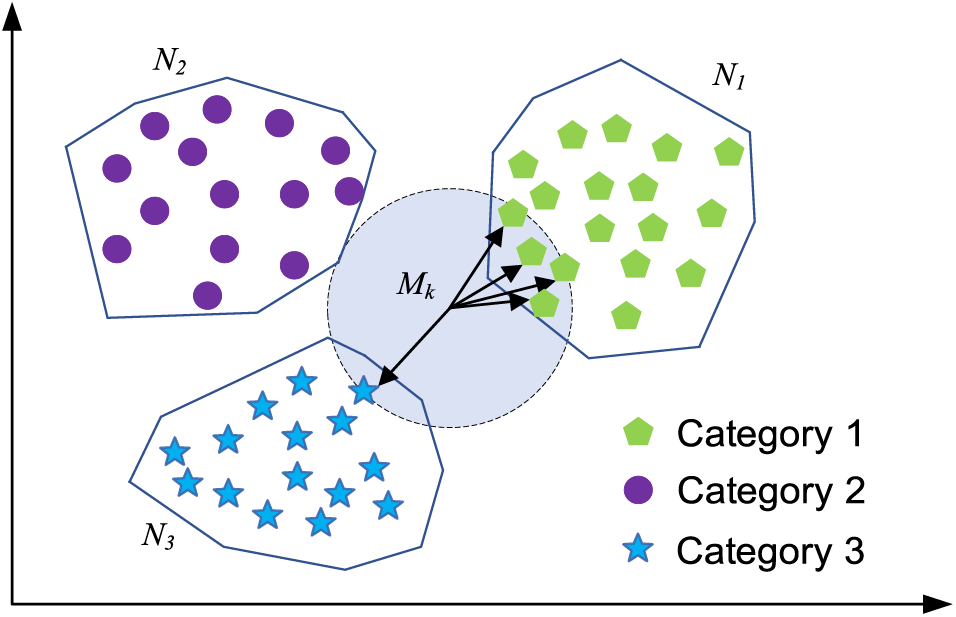
Figure 5: Schematic diagram of the KNN algorithm
According to the basic idea of KNN, determinations of the appropriate k-value and the distance between samples are the core elements of the application of the KNN to address the classification problem.
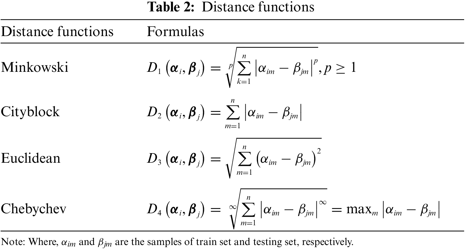
In KNN, the degrees of similarity between the two sample points are usually represented by calculating their distance by using distance function. The shorter the distance, the higher the similarity. Many different types of distance functions are developed, such as Minkowski distance, Euclidean distance, and Chebyshev distance. The selection of the distance function is of utmost importance for achieving high classification accuracy. To investigate the impact of different distance metrics on the KNN classification model, four distance functions are selected to study their influence on the classification results. The selected distance functions are shown in Table 2.
4.1.3 Determination of the K-Value and Distance Function by Cross-Validation Method
The k-value is the only hyperparameter in the KNN algorithm, which has an important influence on the prediction results. When the k-value is small, it means that the classification results are determined only by the categories of the nearest samples in the neighborhood. However, when the training set contains “noise samples”, the model is also susceptible to these noise samples. Then, it may reduce the training error and easily result in overfitting. When the k-value is large, it may reduce estimation errors, but can also easily lead to an increasing of the approximation errors of learning. In practical application, the k-value generally takes a relatively small integer which is not greater than 20.
To determine an optimal k-value, the 10-fold cross-validation method is used. First, the sample data is randomly and equally divided into 10 parts. Then, nine parts of them are treated as training set and one part as a test set on a rotational basis. Finally, the average of the cross-validation accuracy rate of the ten results is treated as the classification accuracy of the KNN algorithm. To reduce the influence of the random division of samples under a 10-fold cross-validation, one hundred 10-fold cross-validations are made and the average accuracy rates of the one hundred 10-fold cross-validations for classification of the DSV fault degrees are obtained. By analyzing the variation law of cross-validations with respect to the k-value and the basic principle of selection of the k-value, the optimal k-value will be determined. The relationship between 10-fold cross-validation average accuracy, k-value, and distance functions is shown in Fig. 6. It can be seen that k = 1 has the highest accuracy rate for each distance function. However, although the accuracy rate of k = 1 is the highest, to avoid the influence of noise, k = 1 will not be selected. As shown in Fig. 6, when k = 5 and the distance function is Chebyshev, the KNN model achieves the second-highest average classification accuracy rate. Based on the above reasons and the results in Fig. 6, to ensure high accuracy of test results and reduce the impact of noise, k = 5 is determined and the Chebyshev distance function is selected.
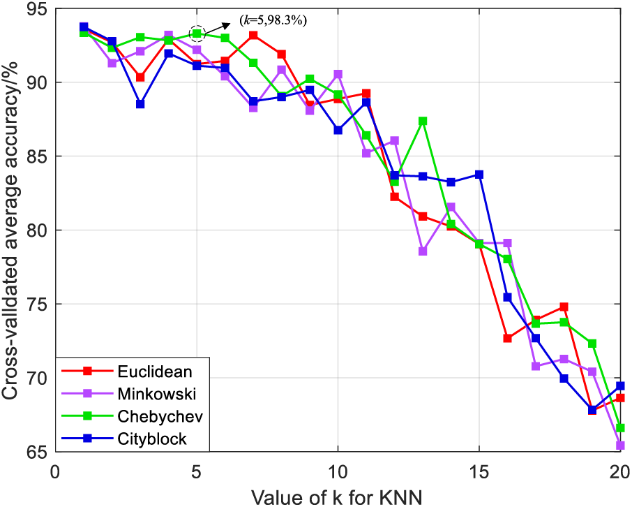
Figure 6: Relationship between 10-fold cross-validation average accuracy, k-value, and distance functions
4.2 Fault Diagnosis and Results Analysis
4.2.1 Application Steps of KNN for Diagnosis of DSV Fault Degrees
In this paper, the KNN model is used to classify the four different degrees of DSV fault. The flow chart of KNN for diagnosis of DSV fault degrees is shown in Fig. 7 and the detailed application procedures are as follows:
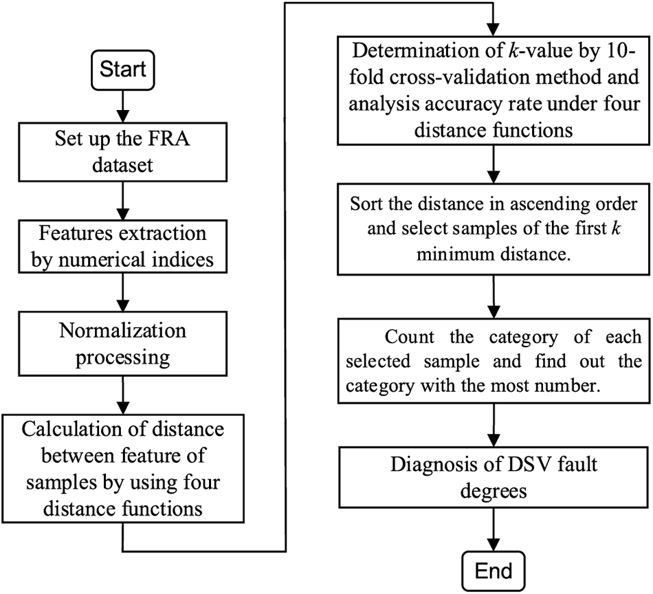
Figure 7: Flow chart of the KNN for diagnosis of DSV fault degrees
1. Set up the FRA dataset. By using the FRA test setup, the FRA fingerprint of healthy winding and the FRA curves of winding with different degrees of DSV fault are measured.
2. Feature extraction. The features existing in the variation of the FRA curves caused by DSV faults are obtained by using the selected numerical indices.
3. Normalization of Features. To eliminate the influence of the dimension of different numerical indices, the Min-Max method is used to normalize the features extracted by numerical indices.
4. Calculation of distance between features by using four distance functions.
5. Determination of the optimal k-value and the best distance function. By evaluating the average accuracy rate of the KNN model under different k-value and distance functions based on the 10-fold cross-validation method, the optimal k-value and the best distance function are determined.
6. Sort the distance in ascending order and select samples of the first k minimum distance.
7. Count the category of each selected sample and find out the category with the most number.
8. Diagnosis of the DSV fault degrees.
9. End.
4.2.2 Results Analysis and Comparison with SVM Algorithm
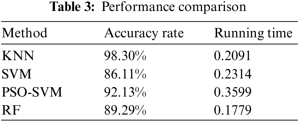
The diagnosis accuracy rate has been obtained in Section 4. The average accuracy rate of the KNN model for the classification of the DSV fault degrees is 98.30%, as shown in Fig. 6. To show the performance of the proposed method, the accuracy rate and running time of the traditional SVM, PSO-SVM, and RF methods are calculated to compare with those of KNN.
The DSV fault degree of the winding model belongs to a small sample, nonlinear, and high-dimensional pattern recognition problem. As a typical machine learning algorithm, SVM has a very strong ability to address this problem and it has good generalization ability in the case of limited samples. In addition to SVM, since the RF algorithm can deal with unstructured data, it can better capture the complex relationship between data, so as to improve the prediction accuracy. Meanwhile, RF is a flexible, easy-to-use machine learning algorithm that produces, even without hyper-parameter tuning. Therefore, to show the performance of the KNN for the classification of DSV fault degrees, it is necessary to compare KNN with SVM, PSO-SVM, and RF algorithms. The radial basis function is used in the SVM and PSO-SVM methods. The number of decision trees and leaf nodes in the RF model are both three. The performance comparison results are shown in Table 3. Although RF is faster than that of KNN, the accuracy rate of RF is the lowest. It can be seen that KNN has the highest accuracy rate among these methods. It means that the KNN is particularly suitable for dealing with multi-classification problems and it performs better than the SVM, PSO-SVM, and RF for the classification of the DSV fault degrees of winding. In addition, since the number of fault samples is relatively small, the running time of the KNN is also better than that of the SVM and PSO-SVM. It needs to state that the running time of the SVM and PSO-SVM models shown in Table 3 also contains the operation time of the 10-fold cross-validation.
In the paper, a diagnosis model which combines KNN and FRA is proposed to diagnose the DSV fault degrees of transformer winding. A lot of FRA tests are performed on a transformer winding model which is set with different degrees of DSV faults to acquire the FRA dataset. A series of numerical indices are selected and used to extract the features existing in the FRA curves. After determining the optimal k-value of KNN and best distance function by using the 10-fold cross-validation method and the distance between features of samples, the KNN model is built and it is used to diagnose the DSV fault degrees of winding. The diagnostic accuracy rate of the proposed model is up to 98.30% which is better than the SVM, PSO-SVM, and RF methods. Additionally, the running time of the proposed model for the classification of the DSV fault degrees of winding is also better than the SVM and PSO-SVM. The diagnosis results show that the proposed model has a good ability to diagnose the DSV fault degrees of winding. The proposed diagnosis method provides a quantitative approach for the fault diagnosis of transformer winding. It has an important practical significance for technical personnel to detect winding deformation and quickly develop a related maintenance strategy. Meanwhile, the contribution of this paper is beneficial to the development of a standard interpretation algorithm for the fault detection of the transformer winding.
In a further study, if conditions permit, the proposed model needs to be applied to some real transformers to further validate its accuracy. In addition, fault types and fault locations of transformer winding both need to be researched based on the proposed model in the future.
Acknowledgement: The authors would like to thank T.L. and C.L. for providing the technical support.
Funding Statement: This work is supported in part by Shaanxi Natural Science Foundation Project (2023-JC-QN-0438), and in part by Fundamental Research Funds for the Central Universities (2452021050).
Author Contributions: Study conception and design: T.L. and C.L.; data collection: F.Y.; analysis and interpretation of results: S.Q.; draft manuscript preparation: F.X. and S.W.; review and editing: S.W. All authors reviewed the results and approved the final version of the manuscript.
Availability of Data and Materials: Not applicable.
Conflicts of Interest: The authors declare that they have no conflicts of interest to report regarding the present study.
References
1. Hamed Samimi, M., Dadashi Ilkhechi, H. (2020). Survey of different sensors employed for the power transformer monitoring. IET Science, Measurement & Technology, 14(1), 1–8. https://doi.org/10.1049/iet-smt.2019.0103 [Google Scholar] [CrossRef]
2. Wang, S., Wang, S., Feng, H., Guo, Z., Wang, S. et al. (2017). A new interpretation of FRA results by sensitivity analysis method of two FRA measurement connection ways. IEEE Transactions on Magnetics, 54(3), 1–4. https://doi.org/10.1109/TMAG.2017.2743986 [Google Scholar] [CrossRef]
3. Florkowski, M., Furgał, J. (2009). Modelling of winding failures identification using the frequency response analysis (FRA) method. Electric Power Systems Research, 79(7), 1069–1075. https://doi.org/10.1016/j.epsr.2009.01.009 [Google Scholar] [CrossRef]
4. Arispe, J. C. G., Mombello, E. E. (2014). Detection of failures within transformers by FRA using multiresolution decomposition. IEEE Transactions on Power Delivery, 29(3), 1127–1137. https://doi.org/10.1109/TPWRD.2014.2306674 [Google Scholar] [CrossRef]
5. Palani, A., Santhi, S., Gopalakrishna, S., Jayashankar, V. (2008). Real-time techniques to measure winding displacement in transformers during short-circuit tests. IEEE Transactions on Power Delivery, 23(2), 726–732. https://doi.org/10.1109/TPWRD.2007.911110 [Google Scholar] [CrossRef]
6. Dobizha, N. E., Pichugina, M. T. (2014). Checking features of the transformer winding mechanical joint conditions by the method of low-voltage impulse. 2014 9th International Forum on Strategic Technology (IFOST), pp. 382–385. Cox’s Bazar, Bangladesh. https://doi.org/10.1109/IFOST.2014.6991145. [Google Scholar] [CrossRef]
7. Ni, J. Q., Zhao, Z. Y., Tan, S., Chen, Y., Yao, C. G. et al. (2020). The actual measurement and analysis of transformer winding deformation fault degrees by FRA using mathematical indicators. Electric Power Systems Research, 184(6), 1–11. https://doi.org/10.1016/j.epsr.2020.106324 [Google Scholar] [CrossRef]
8. Bagheri, S., Moravej, Z., Gharehpetian, G. B. (2018). Classification and discrimination among winding mechanical defects, internal and external electrical faults, and inrush current of transformer. IEEE Transactions on Industrial Informatics, 14(2), 484–493. https://doi.org/10.1109/TII.2017.2720691 [Google Scholar] [CrossRef]
9. Samimi, M. H., Hillenbrand, P., Tenbohlen, S., Shayegani Akmal, A. A., Mohseni, H. et al. (2019). Investigating the applicability of the finite integration technique for studying the frequency response of the transformer winding. International Journal of Electrical Power & Energy Systems, 110(1), 411–418. https://doi.org/10.1016/j.ijepes.2019.03.015 [Google Scholar] [CrossRef]
10. Sofian, D. M., Wang, Z., Li, J. (2010). Interpretation of transformer FRA responses—Part II: Influence of transformer structure. IEEE Transactions on Power Delivery, 25(4), 2582–2589. https://doi.org/10.1109/TPWRD.2010.2050342 [Google Scholar] [CrossRef]
11. Samimi, M. H., Tenbohlen, S. (2017). FRA interpretation using numerical indices: State-of-the-art. International Journal of Electrical Power & Energy Systems, 89(6), 115–125. https://doi.org/10.1016/j.ijepes.2017.01.014 [Google Scholar] [CrossRef]
12. Rahimpour, E., Jabbari, M., Tenbohlen, S. (2010). Mathematical comparison methods to assess transfer functions of transformers to detect different types of mechanical faults. IEEE transactions on Power Delivery, 25(4), 2544–2555. https://doi.org/10.1109/TPWRD.2010.2054840 [Google Scholar] [CrossRef]
13. Liu, J., Zhao, Z., Tang, C., Yao, C., Li, C. et al. (2019). Classifying transformer winding deformation fault types and degrees using FRA based on support vector machine. IEEE Access, 7, 112494–112504. https://doi.org/10.1109/ACCESS.2019.2932497 [Google Scholar] [CrossRef]
14. Bigdeli, M., Vakilian, M., Rahimpour, E. (2012). Transformer winding faults classification based on transfer function analysis by support vector machine. IET Electric Power Applications, 6(5), 268–276. https://doi.org/10.1049/iet-epa.2011.0232 [Google Scholar] [CrossRef]
15. Mao, X., Wang, Z., Crossley, P., Jarman, P., Fieldsend-Roxborough, A. et al. (2020). Transformer winding type recognition based on FRA data and a support vector machine model. High Voltage, 5(6), 704–715. https://doi.org/10.1049/hve.2019.0294 [Google Scholar] [CrossRef]
16. Luo, Y., Ye, J., Gao, J., Chen, G., Wang, G. et al. (2017). Recognition technology of winding deformation based on principal components of transfer function characteristics and artificial neural network. IEEE Transactions on Dielectrics and Electrical Insulation, 24(6), 3922–3932. https://doi.org/10.1109/TDEI.2017.006655 [Google Scholar] [CrossRef]
17. Mao, X., Ji, S., Wang, Z., Jarman, P., Fieldsend-Roxborough, A. et al. (2020). Applying unsupervised machine learning method on FRA data to classify winding types. Proceedings of the 21st International Symposium on High Voltage Engineering, vol. 1, pp. 969–981. Budapest, Hungary. https://doi.org/10.1007/978-3-030-31676-1_91 [Google Scholar] [CrossRef]
18. IEEE Standard C57.149 (2012). IEEE guide for the application and interpretation of frequency response analysis for oil-immersed transformers. https://doi.org/10.1109/IEEESTD.2013.6475950 [Google Scholar] [CrossRef]
19. IEC Standard on Power Transformers (2012). Part 18: Measurement of frequency response. Standard IEC 60076-18. https://infostore.saiglobal.com/en-au/Standards/Product-Details-1109398_SAIG_VDE_VDE_2578726/?productID=1109398_SAIG_VDE_VDE_2578726 [Google Scholar]
20. Tahir, M., Tenbohlen, S., Samimi, M. H. (2020). Evaluation of numerical indices for objective interpretation of frequency response to detect mechanical faults in power transformers. Proceedings of the 21st International Symposium on High Voltage Engineering, 1, 811–824. https://doi.org/10.1007/978-3-030-31676-1 [Google Scholar] [CrossRef]
21. Pourhossein, K., Gharehpetian, G. B., Rahimpour, E., Araabi, B. N. (2012). A probabilistic feature to determine type and extent of winding mechanical defects in power transformers. Electric Power Systems Research, 82(1), 1–10. https://doi.org/10.1016/j.epsr.2011.08.010 [Google Scholar] [CrossRef]
22. Ghanizadeh, A. J., Gharehpetian, G. B. (2014). ANN and cross-correlation based features for discrimination between electrical and mechanical defects and their localization in transformer winding. IEEE Transactions on Dielectrics and Electrical Insulation, 21(5), 2374–2382. https://doi.org/10.1109/TDEI.2014.004364 [Google Scholar] [CrossRef]
23. Samimi, M. H., Tenbohlen, S. (2016). The numerical indices proposed for the interpretation of the FRA results: A review. VDE High Voltage Technology 2016; ETG-Symposium, pp. 1–7. Berlin, Germany. [Google Scholar]
24. Kim, J. W., Park, B., Jeong, S. C., Kim, S. W. et al. (2005). Fault diagnosis of a power transformer using an improved frequency-response analysis. IEEE Transactions on Power Delivery, 20(1), 169–178. https://doi.org/10.1109/TPWRD.2004.835428 [Google Scholar] [CrossRef]
25. Badgujar, K. P., Maoyafikuddin, M., Kulkarni, S. V. (2012). Alternative statistical techniques for aiding SFRA diagnostics in transformers. IET Generation, Transmission & Distribution, 6(3), 189–198. https://doi.org/10.1049/iet-gtd.2011.0268 [Google Scholar] [CrossRef]
26. Behjat, V., Mahvi, M. (2015). Statistical approach for interpretation of power transformers frequency response analysis results. IET Science, Measurement & Technology, 9(3), 367–375. https://doi.org/10.1049/iet-smt.2014.0097 [Google Scholar] [CrossRef]
27. Kennedy, G. M., McGrail, A. J., Lapworth, J. A. (2007). Using cross-correlation coefficients to analyze transformer sweep frequency response analysis (SFRA) traces. IEEE Power Engineering Society Conference and Exposition in Africa-Power Africa, pp. 1–6. Johannesburg, South Africa. https://doi.org/10.1109/PESAFR.2007.4498059 [Google Scholar] [CrossRef]
28. Karimifard, P., Gharehpetian, G. B., Tenbohlen, S. (2008). Determination of axial displacement extent based on transformer winding transfer function estimation using vector-fitting method. European Transactions on Electrical Power, 18(4), 423–436. https://doi.org/10.1002/(ISSN)1546-3109 [Google Scholar] [CrossRef]
Cite This Article
 Copyright © 2023 The Author(s). Published by Tech Science Press.
This work is licensed under a Creative Commons Attribution 4.0 International License , which permits unrestricted use, distribution, and reproduction in any medium, provided the original work is properly cited.
 Downloads
 Citation Tools