Parallel Integrated Model-Driven and Data-Driven Online Transient Stability Assessment Method for Power System

1  Introduction

Online transient stability assessment is the basis to ensure the safe operation of the power system. In recent years, the large-scale grid connection of high-proportion renewable energy has aggravated the complexity of the power system, which makes the online transient stability assessment face new challenges.

The existing power system transient stability assessment methods are mainly divided into two categories: model-driven methods and data-driven methods.

The model-driven methods first establish the physical mechanism models described by differential-algebraic equations according to the physical characteristics of power systems and then assess the transient stability by solving the mechanism models through mathematical methods, including the time domain simulation method and the direct methods. The time domain simulation method [1] takes the steady-state power flow as the initial value, solves the state equations by numerical integration method to get the disturbed trajectory of the power system, and then determines its transient stability, which is the basic method for assessing the transient stability. The calculation results of the time domain simulation method are accurate and reliable, but the calculation process takes a long time and is slow, so this method is difficult to be applied online. The direct methods (including the energy function method [2], BCU method [3], extended equal area criterion (EEAC) method [4], rate of change of kinetic energy method [5], etc.) are based on Lyapunov stability theory, and the transient stability is determined by distinguishing the time-varying of the constructed energy functions. Because the direct methods do not need the numerical integral calculation of the whole transient process, the calculation speed is quite fast, and it can be applied to the online assessment of transient stability. In addition, it is worth noting that the authors in reference [6] proposed a novel direct method for online transient stability assessment, which combines equal area criterion, corrected kinetic energy, and large change sensitively analysis, and this method not only considers all details of power systems by using network preserving models but also achieves simplicity in implementation and low computational cost.

In recent years, the data-driven methods that learn the transient characteristics of power systems through data statistics and various machine learning algorithms have been successfully applied to transient stability assessment. With the wide applications of new energy technologies (such as electric vehicle charging technology and demand response technology), the power system contains more and more uncertainties, and the traditional model-driven methods cannot cope with these uncertainties well. With the increasing complexity of power system structures and operation modes, the model-driven methods need to adjust the models according to different scenarios, structures, and operation modes. The higher calculation cost and slower calculation speed make their adaptability worse. On the contrary, the data-driven methods employ a series of data tricks (including data preprocessing, data transformation, spatial mapping, etc.), and various modern advanced machine learning algorithms (including support vector machine [7–9], Bayesian method [10], decision tree method [11,12], random forest method [13,14], deep learning method [15–21], active learning method [22], etc.) to seek the valuable information from the data, and obtain the assessment results of the transient stability. The data-driven methods can get rid of the dependence on complex physical mechanism models, and have the advantages of dealing with uncertain factors and fast calculation speed. However, the data-driven methods also have some drawbacks in the application, i.e., the assessment results lack interpretation, and the generalization ability is low.

It can be seen that integrating the model-driven methods and the data-driven methods by taking full advantage of their complementary properties are the future development trends for power system online transient stability assessment. At present, researchers have carried out some research in this area, and almost all of them have adopted the “serial integrated” pattern (that is, using the knowledge rules derived from model-driven methods to modify the objective functions of data-driven methods [23–25]) to achieve the purpose of improving the accuracy of the assessment results. The schematic diagram of these “serial integrated” methods is shown in Fig. 1. These serial integrated methods firstly extract the original high dimensional input features of power systems efficiently through physical mechanism models, and then the data methods are used to directly adjust the output results of physical models, to realize the coordination between model-driven and data-driven methods. The serial integrated methods are relatively easy to implement because the input/output interfaces of data-driven methods are always designed to be open. However, some unavoidable uncertainties still exist in the output results of these serial integrated methods due to the employed framework.

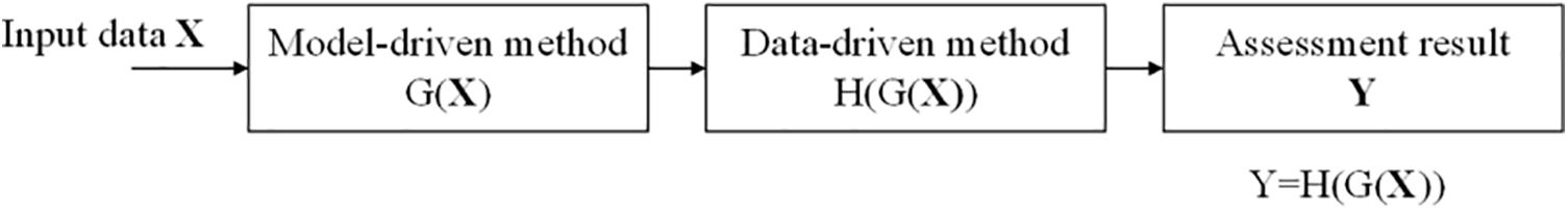
Figure 1: Schematic diagram of the “serial integrated” method

Compared to the “serial integrated” pattern, the “parallel integrated” pattern is obviously more robust and it can obtain a more definite (to some extent, more reliable) transient stability assessment result. The key challenge of parallel integrated methods is to construct a reasonable function that directly links model-driven and data-driven methods. Considering the great robustness of the “parallel integrated” pattern, this paper proposes a new “parallel integrated” method, which combines model-driven methods and data-driven methods to assess the transient stability of the power system. In the model-driven stage, the rate of change of kinetic energy method is used to determine the transient stability by calculating the critical clearing time of faults, because this method does not need the numerical integral calculation of the whole transient process and has a strict theoretical basis, fast calculation speed, and reliable results. In the data-driven stage, the support vector machine algorithm and the extreme learning machine algorithm with different internal principles are respectively used to assess the transient stability. In order to quantify the credibility level of data-driven methods, the credibility index of the output results is proposed. Then the switching function which controls whether the rate of change of the kinetic energy method is activated or not is established based on this index. Finally, a new parallel integrated model-driven and data-driven online transient stability assessment method is proposed.

2  Model-Driven Rate of Change of Kinetic Energy Method

The model-driven rate of change of kinetic energy (RCKE) method is introduced, as below. The classical model is used to analyze the transient stability of a multi-machine power system. For the ith generator, the rotor motion equation is

dδidt=ωi(1)

dωidt=1Mi(Pmi−Pei)(2)

where δi is the angle of the rotor; ωi is the angular velocity of the rotor; Mi is the moment of inertia of the generator; Pmi is the mechanical power of the prime mover; Pei is the electromagnetic power of the generator, which can be expressed as

Pei=Ei2Gii+∑j=1j≠in⁡EiEjYijcos(θij−δi+δj)(3)

where Ei is the voltage behind the transient reactance of the generator; Gii is the self-conductance of the internal node of the generator; Yij is the transfer admittance between internal nodes of the generators; θij is the angle corresponding to Yij; n is the total number of generators.

The kinetic energy Wi of the ith generator can be expressed as

Wi=12Miωi2(4)

The rate of change of kinetic energy Pki of the ith generator can be obtained by taking the derivative of time on both sides of the equation, as follows:

Pki=dWidt=Miωidωidt(5)

Substitute Eq. (2) into Eq. (5) to obtain

Pki=ωi(Pmi−Pei)(6)

When the fault is cleared, according to the power network configuration after the fault, the rate of change of kinetic energy can be expressed as

Pki=ωic(Pmi−Pei)(7)

Eq. (7) describes how the kinetic energy of the generator caused by the fault is absorbed and converted into the potential energy of the system. When the system is about to lose its transient stability, at least one generator will lose synchronization. It can be considered that the instability process of the system is caused by an equivalent “key” generator, and the RCKE of the key generator has a negative maximum at the critical clearing time [26]. Thus, the key generator, together with the rest of the system, constitutes a single-machine infinite bus system.

Therefore, the RCKE method can be used to assess the transient stability of the multi-machine power system, and its steps are as follows [5], and the flow chart is given in Fig. 2:

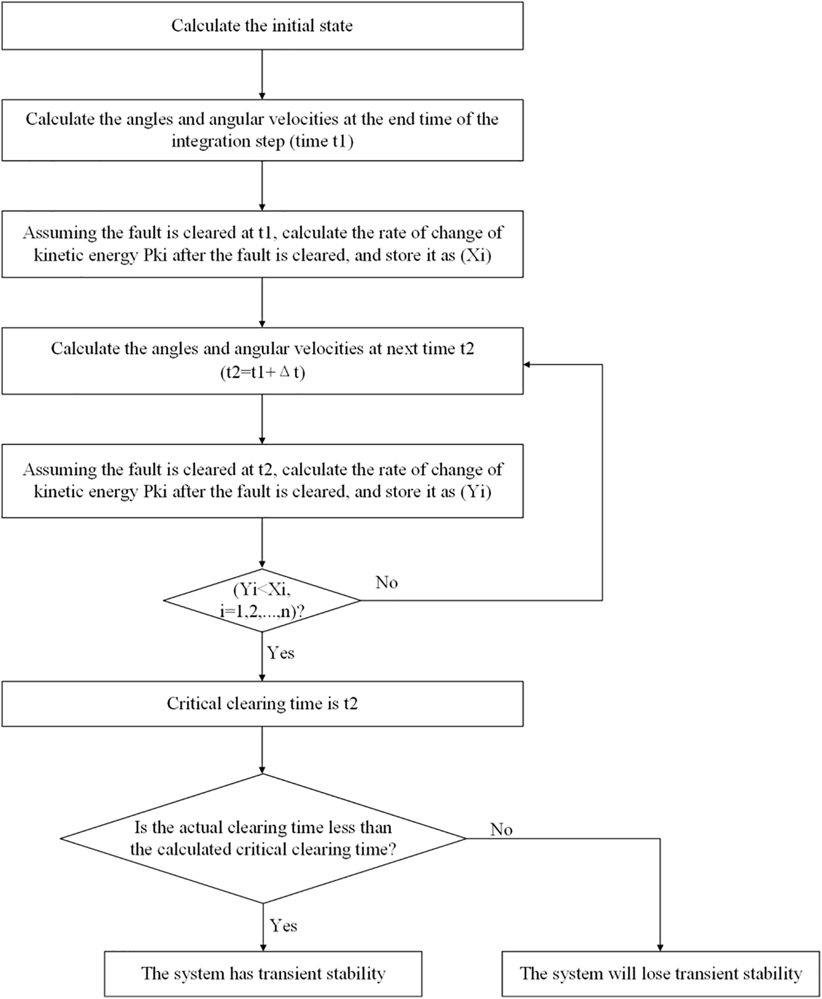
Figure 2: Flow chart of rate of change of kinetic energy method

Step 1. Use the power flow data before the fault to calculate the initial state of the multi-machine power system.

Step 2. The differential-algebraic equations corresponding to the classical model during the fault period are solved by the numerical integration method, and the angles and angular velocities of each generator rotor at the end time of the integration step (time t1) are calculated.

Step 3. Assuming that the fault is cleared at time t1, calculate the rate of change of kinetic energy Pki of each generator after the fault is cleared, i=1,2,…,n and store it as (Xi).

Step 4. Calculate the angle and angular velocity of each generator rotor at the next time t2 (time t2=t1+Δt, where Δt is the integration step) by using the numerical integration method.

Step 5. Assuming that the fault is cleared at the new time t2, calculate the rate of change of kinetic energy Pki of each generator after the fault is cleared, i=1,2,…,n, and store it as (Yi).

Step 6. If there is Yi<Xi, i=1,2,…,n in the amplitude, then the corresponding time t2 is the critical clearing time; otherwise, let Xi=Yi, and perform Step 4 to Step 6 again.

Step 7. If the actual fault clearing time of the system is less than the critical clearing time obtained above, the system has transient stability; otherwise, the system will lose transient stability.

3  Data-Driven Machine Learning Method

3.1 Support Vector Machine

The Support Vector Machine (SVM) classifier is a nonparametric machine learning algorithm, which does not need to assume prior knowledge. The basic idea of SVM is to map the input vector from the sample space to the feature space, find an optimal hyperplane in the feature space, and separate the two types of samples to maximize the separation distance. SVM uses “input-output” (i.e., “feature-label”) data pairs for training to obtain a decision function that can correctly classify a given input quantity into its corresponding label class. This optimal decision function is called the optimal hyperplane and is determined by a small number of vectors in the training data set (called “support vectors”).

For a binary classification problem, given a series of “feature-label” data pairs (xi,yi), i=1,2,…,n, where xi is an m-dimensional column vector which represents the input characteristics of the ith sample; yi∈{1,−1} is the classification label of the ith sample (for example, y=1 indicates transient stability and y=−1 indicates transient instability). Taking the given data pair as the training data set, the SVM can be expressed as the optimization model [7] shown in the following formula:

minw,b,ξ12wTw+C∑i=1nξi

s.t.yi(wTϕ(xi)+b)≥1−ξi,i=1,2,…,n(8)

ξi≥0,i=1,2,…,n

where w is an m-dimensional weighted column vector; b is a constant representing the offset term; ξi is the relaxation variable corresponding to xi, which represents the tolerance of sample classification errors; C is the margin parameter, also known as the penalty factor, which represents the degree of punishment for sample classification errors; ϕ(x) is a high-dimensional function that maps the vector x from the original space to the characteristic space, and is usually called “kernel function”. There are many different types of kernel functions, among which the radial basis function can approximate any function with any error, and there is only one undetermined parameter, which applies to both large and small samples [8]. Therefore, the radial basis kernel function is adopted in this paper, and its expression is

ϕ(xi,xj)=exp(−γ‖xi−xj‖2)(9)

where γ is the kernel parameter.

The values of w, b, and ξi can be obtained by solving the optimization model shown in Eq. (8), while the values of parameters C and γ need to be calculated by grid search or heuristic algorithms.

3.2 Extreme Learning Machine

The Extreme Learning Machine (ELM) classifier is a machine learning algorithm based on a single hidden layer feedforward neural network. When it is used to solve the binary classification problem, the structure of ELM is shown in Fig. 3. As can be seen from Fig. 3, ELM consists of the input layer, hidden layer and output layer. Among them, the input layer has N nodes, corresponding to the dimension of each input vector; there are L nodes in the hidden layer; and the output layer has one node, which corresponds to the output variable. When the network structure is determined in the training stage, ELM does not need to solve it iteratively like the traditional artificial neural network algorithm but only needs to calculate the linear matrix to determine the network structure and parameters, so it has a faster training speed.

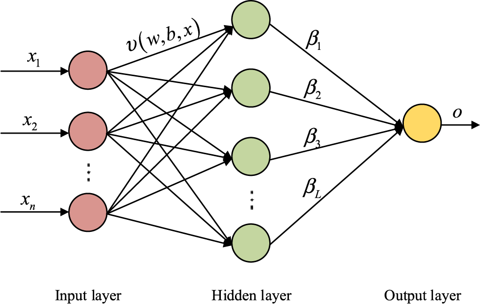
Figure 3: Structure of extreme learning machine

Similar to SVM, a given series of “feature-label” data pairs (xi,yi), i=1,2,…,n (where xi is an m-dimensional column vector; yi∈{1,−1}) as the training data set of ELM, then ELM can be expressed as the following optimization model [21]:

min ∑j=1n‖oj−yj‖s.t.∑i=1Lβiϑ(wiTxj+bi)=oj,j=1,2,…,n(10)

where wi is an m-dimensional weighted column vector, which links the input features represented by the input vector with the ith hidden node; bi is the offset term of the ith hidden node; ϑ(x) is the activation function; βi is the output weight, which links the ith hidden node with the output node.

Because the activation function is infinitely differentiable, βi will be the only parameter to be solved when wi and bi are randomly initialized. Introduce vector β, o and matrix H as follows:

β=[β1,β2,…,βL]T(11)

o=[o1,o2,…,on]T(12)

H=[υ(w1Tx1+b1)υ(w2Tx1+b2)⋯υ(wLTx1+bL)υ(w1Tx2+b1)υ(w2Tx2+b2)⋯υ(wLTx2+bL)⋮⋮⋱⋮υ(w1Txn+b1)υ(w2Txn+b2)⋯υ(wLTxn+bL)](13)

Then, according to the matrix theory, by solving Moore-Penrose generalized inverse matrix H+ of matrix H, the least square solution of vector β can be obtained [27], as follows:

β^=H+o(14)

After the training of the ELM classifier is completed, for a certain sample (x,y) to be classified, x is taken as the input of the ELM classifier, and its output o is obtained. If o≥0, then y=1; If o<0, then y=−1.

3.3 Original Input Features

The selection of original input features has a significant impact on the output results of the machine learning algorithms. In this paper, a large number of samples in different fault scenarios are first generated by time domain simulation. Considering the configurations of Wide Area Measurement Systems (WAMS) in the practical power grids are usually limited, at the same time, in order to correspond to the input information used in the model-driven RCKE method adopted in this paper, the fault information (including fault type, fault location, and fault duration) and the power flow quantities before the fault occurs are taken as the original input features of each sample, which are summarized as follows (as shown in Table 1). It should be pointed out that the fault type and fault location are discrete variables, while all the rest are continuous variables. All these data except the fault duration actually represent the initial state of the transient process of the power system, and the transient stability result can be inferred if all these data are treated as known variables. That is why the power flow information before the fault occurs (other than after the fault occurs) is chosen as the original input feature.

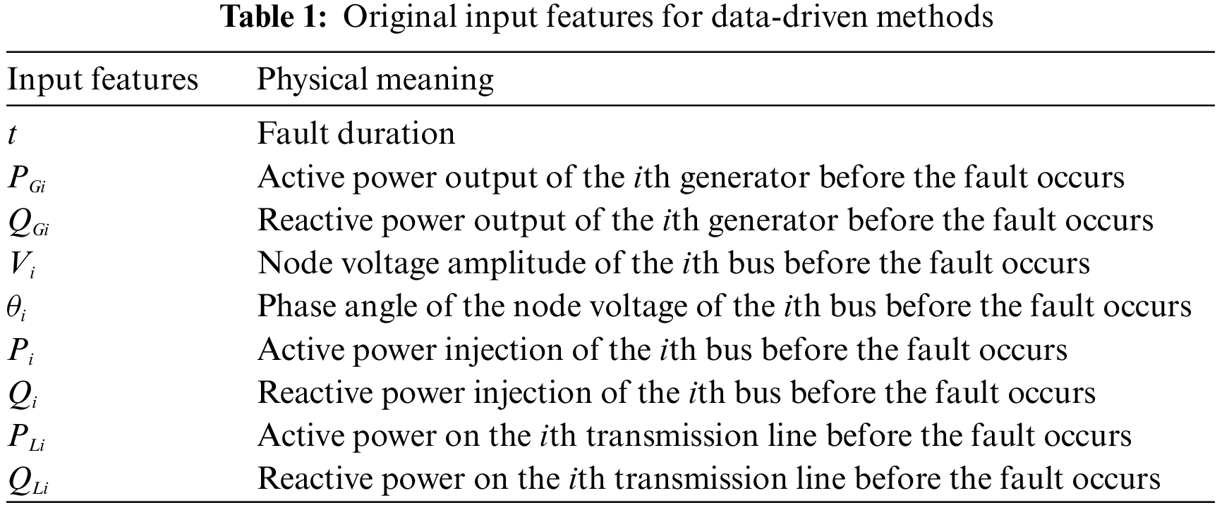
It can be seen from Table 1 that these original input features are directly related to the transient stability of the power system. However, in practical application, the Fisher discriminant method or Pearson correlation coefficient method [28] should be used to calculate the impact coefficient of each original input feature quantity on the final output result, and then only the input feature quantities with significant influence on the output result should be selected so as to improve the robustness of data-driven methods.

Moreover, because the features used above have different dimensions, the features of the order of magnitude difference are relatively large. In order to avoid the model biased in learning large order of magnitude data features, and in order to speed up the convergence of the algorithm, it is necessary to normalize the original input data. Let the sample data matrix D=[xij]n×N, where n is the number of samples, N is the number of features, xij represents the jth feature of the ith sample. Then the normalization formula is as below:

xij∗=xij−mini(xij)maxi(xij)−mini(xij)(15)

The data after normalization is mapped to the range of [0, 1], and can be used as input for the classifiers.

4  Parallel Integrated Model-Driven and Data-Driven Method

As mentioned above, the model-driven methods which are based on mechanism analysis have the advantages of clear mechanism, good interpretability, and high adaptability, while they also have modeling difficulties and low computational efficiency, especially for complex power systems. On the contrary, the data-driven methods which are based on correlation analysis between large data have the advantages of high computational efficiency and a strong ability to deal with complex problems, while their output results lack interpretability. Furthermore, the model-driven methods are deterministic methods, while the output results of data-driven methods always contain some uncertainties inevitably. To be exact, when the model-driven methods and the data-driven methods are respectively used to predict the transient stability of the power system with a certain initial state, the prediction results of the model-driven methods are always definite, while the prediction results of the data-driven methods are uncertain because they are affected by the quality of input data and the trained parameters of classifiers. Roughly speaking, the model-driven methods are trustworthy but inefficient, while the data-driven methods are not trustworthy enough but efficient. Therefore, it is reasonable to combine these two kinds of methods to get better output results by taking full advantage of their complementary properties.

This paper proposes a new “parallel mode” to integrate these two kinds of methods, and the feasibility analysis is given as below. The basic idea of the proposed method is when the output result of the data-driven method is comparatively reliable we do not turn to the model-driven method otherwise we must turn to the model-driven method. More specifically, two independent classifiers (i.e., SVM classifier and ELM classifier) are employed in the data-driven stage to predict the transient stability of the power system, and the model-driven stage employs the RCKE method. For each classifier in machine learning, its credibility level can be evaluated because its output result is determined through the demarcation point. Intuitively, the longer the distance between a sample to be classified and the demarcation point, the higher the credibility level of the output result of this classifier for this sample will be. Based on this observation, a “switching function” which comprehensively reflects the credibility level of these two independent classifiers is established. If the switching function holds, it indicates that the data-driven stage ends in failure because its credibility level does not meet the preset quantitative criteria, and we must turn to the model-driven method, otherwise, we do not turn to the model-driven method. Therefore, it is feasible to combine these two kinds of methods by the proposed parallel mode.

4.1 Accuracy Evaluation of Classifiers

In the practical operation of a power system, the ratio of actual stable samples to actual unstable samples is unbalanced. In order to evaluate the accuracy of the classifiers’ prediction results, it is necessary to introduce the confusion matrix (as shown in Table 2), and then define the relevant indicators of accuracy. In Table 2, TP and TN respectively represent the number of samples accurately predicted by the classifiers as stable and unstable, FP represents the number of unstable samples missed by the classifiers, and FN represents the number of stable samples misjudged by the classifiers. Let NP and NN represent the total number of samples that are actually stable and unstable, respectively, then NP=TP+FN and NN=FP+TN.

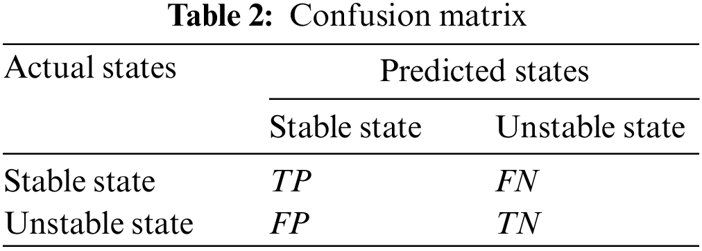
According to Table 2, the following five indexes can be defined to comprehensively reflect the accuracy of the classifiers in predicting transient stability.

The Accuracy Rate (AR) index refers to the ratio of the number of accurately predicted samples to the total number of samples, as follows:

AR=(TP+TN)/(NP+NN)×100%(16)

The Reliability Rate (RR) index indicates the ratio of the number of samples accurately predicted by the classifiers to the total number of samples that are actually unstable, as follows:

RR=TN/NN×100%(17)

The Safety Rate (SR) index indicates the ratio of the number of samples accurately predicted by the classifiers to the total number of samples that are actually stable, as follows:

SR=TP/NP×100%(18)

The Missed Detection Rate (MDR) index indicates the ratio of the number of unstable samples missed by the classifiers to the total number of samples, as follows:

MDR=FP/(NP+NN)×100%(19)

The False Alarm Rate (FAR) indicates the ratio of the number of stable samples misjudged by the classifiers to the total number of samples, as follows:

FAR=FN/(NP+NN)×100%(20)

If we misjudge the unstable samples as stable and do not take any measures, it can lead to disastrous results, which must be avoided. On the other hand, if there is a large number of stable samples which are misjudged as unstable, the assessment results will be too conservative. Therefore, when evaluating the performance of different classifiers, we should first try to reduce the number of unstable samples missed by classifiers FP, and use RR as the main index (the higher the better); use AR as a secondary evaluation index. If a large number of stable samples are judged to be unstable, FP will decrease, but FN will increase which means that the transient stability control devices will be frequently triggered.

4.2 Credibility Evaluation of Classifiers

4.2.1 Credibility Evaluation of SVM Classifier

When the optimization model shown in Eq. (8) is solved, the optimal hyperplane found is

wTϕ(x)+b=0(21)

For a sample (x,y) to be classified, let

g(x)=wTϕ(x)+b(22)

Then the magnitude of g(x) reflects the distance between the sample x and the optimal classification hyperplane, and the sign of g(x) indicates which side of the optimal classification hyperplane the sample x is located on.

The longer the distance between a sample to be classified and the optimal classification hyperplane, the higher the credibility of the classification result of the SVM classifier for this sample will be. When a sample to be classified is closer to the optimal hyperplane, it should be considered that the credibility of the classification result of the SVM classifier for this sample is lower. In this paper, by introducing the Sigmoid function, the distance between the sample to be classified and the optimal hyperplane is mapped into the interval [0, 1], i.e.,

P(C1|x)=1/(1+exp(−g(x)))(23)

P(C−1|x)=1/(1+exp(g(x)))(24)

where P(C1|x) and P(C−1|x) respectively represent the probability that the sample x to be classified is classified into Class 1 and Class -1 by the SVM classifier.

The Eqs. (12) and (13) are added together to obtain

P(C1|x)+P(C−1|x)=100%(25)

Therefore, the credibility index of the classification result of the SVM classifier for the sample x can be defined as

R1=max{P(C1|x),P(C−1|x)}(26)

For the binary classification problem in transient stability prediction, the credibility index R1 ranges from 50% to 100%. When R1 is 50%, it represents that the distance between the sample x and the optimal classification hyperplane is zero, and the probabilities of being classified into Class 1 and Class -1 are equal, i.e., the credibility of the transient stability prediction is 50%.

4.2.2 Credibility Evaluation of ELM Classifier

For a given sample (x,y) to be classified, take x as the input of the ELM classifier, and obtain its output o. Similar to the SVM classifier, when the output o of the ELM classifier is close to the critical point of classification (i.e., 0), its transient stability prediction result will be highly uncredible [29]. Therefore, we can still use the Sigmoid function to evaluate the credibility of the ELM classifier. The credibility R2 of the classification result of the ELM classifier for the sample x can be defined as

R2=max{1/(1+exp(−o)),1/(1+exp(o))}(27)

4.3 Relation between Accuracy and Credibility

The accuracy indexes and credibility indexes of the SVM classifier and ELM classifier have been established, as above. In order to comprehensively evaluate the performance of the classifiers, the relation between accuracy and credibility can be obtained by using statistical analysis for the performance of the classifiers applying to the samples in testing sets. For illustration, the relation between the accuracy rate index and credibility index of the SVM classifier is shown in Fig. 4, as follows.

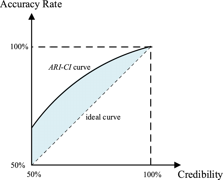
Figure 4: Relation between accuracy rate and credibility of SVM classifier

As can be seen, the abscissa axis is the credibility index (CI) defined in Eq. (26), and the vertical axis is the accuracy rate index (ARI) defined in Eq. (16). The plotted ARI-CI curve can reflect the relation between the accuracy and credibility of the SVM classifier. Under a random guess situation, when CI is 50%, ARI is 50% too (because if ARI is less than 50%, the result is worse than a random guess, which means failed classification). With the increase of CI, ARI of the SVM classifier will also increase. The ideal ARI-CI curve is shown as the plotted dotted diagonal line, which means the classification accuracy of samples (which are 100% credible) should also be 100%.

4.4 Cross-Validation of Classifiers

In the process of applying the classifiers, the data is generally divided into two parts, which are respectively used for training and testing to verify the validity of the classifiers. The common validation methods include simple validation and cross-validation. A simple validation is to take a certain proportion of data from the original data as the number of tests. However, the randomness of test set selection will affect the final results.

Therefore, it is better to use cross-validation, and the basic idea is to divide the data into N groups randomly where each subset of data is used as a test set, and the other N − 1 groups are used as the training sets to build the classifier. A total of N experiments are performed, and the average values of the performance indexes (including accuracy indexes and credibility indexes) are obtained to comprehensively evaluate the classifiers. Cross-validation can eliminate the random selection of training sets, and avoid over-learning and under-learning effectively. In this paper, 5-fold cross-validation is used for applying the classifiers.

4.5 Scheme of Proposed Parallel Integrated Model-Driven and Data-Driven Method

When the model-driven RCKE method is used for transient stability prediction, the prediction result is always determined because the adopted physical mechanism model itself is determined, that is, the accuracy and credibility of the prediction result of the RCKE method can be considered as 100%.

On the contrary, in the process of applying the data-driven methods, because of their “black-box” properties and poor interpretability, the accuracy evaluation and credibility evaluation of their output results must be investigated, respectively.

This paper proposes a new parallel mode to integrate the model-driven and data-driven method, and the mechanism of the proposed method is clarified as below. Generally speaking, the model-driven methods utilize the physical mechanisms of a power system to infer its characteristics, construct corresponding detailed physical models to describe the relationship between the feature domain and the target domain, and establish the mapping from power system features 𝒳1 to output results 𝒴, i.e., ℱ:𝒳1→𝒴. The data-driven methods avoid complex analysis of internal mechanisms, reflect the power system characteristics through a large number of data tests and experiments, and use different data processing algorithms to construct the relationship between the feature domain and the target domain, and establish the mapping from power system features 𝒳2 to output results 𝒴, i.e., 𝒢:𝒳2→𝒴. The diagram of the proposed parallel integrated method is shown in Fig. 5, where ℋ is the proposed “switching function” and it controls whether the model-driven method should be activated or not. Two independent classifiers (i.e., SVM classifier and ELM classifier) are employed in the data-driven stage, because they both output the same transient stability assessment result usually means the output result is quite reliable. More specifically, combined with the credibility evaluation of the single classifier which is given in Sections 4.2 and 4.3, the switching function is constructed by introducing a credibility threshold. Thus, the model-driven method and date-driven method are integrated, and the steps are as follows.

Figure 5: Schematic diagram of the proposed parallel integrated method

Firstly, after collecting data (such as load level, power network structure, and fault set) and generating sample data sets by time domain simulation method, the sample sets are randomly divided into training set 1 and testing set 1 for the SVM classifier. For the ELM classifier, the sample sets are randomly divided into training set 2 and testing set 2. This is to ensure that the SVM classifier and ELM classifier are independent of each other. The five accuracy indexes proposed in this paper are used to comprehensively evaluate the accuracy of the two classifiers. If the accuracy of SVM or ELM does not meet the requirements, it is necessary to reset the parameters, train, and test.

Secondly, after the training of the two classifiers is completed and their accuracy meets the requirements, they can be used for online transient stability prediction. And the prediction result in Z1, credibility index R1, the prediction result in Z2, and credibility index R2 can be obtained, respectively. By setting the credibility threshold Rth (for example, Rth=90%), the case-by-case discussion can be conducted according to the credibility evaluation of the two classifiers.

When the prediction results in Z1 and Z2 are different, the corresponding credibility indexes R1 and R2 have the following four situations.

{R1≥Rth,R2≥RthR1≥Rth,R2<RthR1<Rth,R2≥RthR1<Rth,R2<Rth(28)

It can be seen that when R1≥Rth and R2<Rth, the prediction result Z1 should be adopted; when R1<Rth, R2≥Rth, the prediction result Z2 should be adopted; and the other two situations mean that the data-driven methods fail to predict, and it is necessary to use the model-driven method to predict.

When the prediction results in Z1 and Z2 are the same, the corresponding credibility indexes R1 and R2 also have four situations as shown in Eq. (26). It can be seen that only when R1<Rth, R2<Rth, the model-driven method needs to be used for prediction, while under the other three situations, we can directly output the prediction result Z1 as the final result.

Therefore, the switching function which controls whether the model-driven RCKE method is activated or not can be constructed as follows:

(R1≥Rth&&R2≥Rth)∥(R1<Rth&&R2<Rth)==True(29)

(R1<Rth&&R2<Rth)==True(30)

When Eqs. (29) or (30) is satisfied, it indicates that the data-driven methods end in failure, and the model-driven RCKE method must be used for prediction. Otherwise, it means that the credibility of the data-driven methods meets the requirements, and their prediction results can be directly used as the final output results.

In conclusion, when the model-driven methods and data-driven methods are used to predict the transient stability of a multi-machine power system in the same initial state, the accuracy and credibility of the output results of the model-driven methods are high, but the calculation efficiency is relatively low. The data-driven methods have high computation efficiency, but the accuracy and credibility of their output results are relatively low. Based on the proposed switching function controlling whether the model-driven RCKE method is activated or not, this paper suggests a new parallel integrated model-driven and data-driven online transient stability assessment method, and the flow chart of this proposed method is shown in Fig. 6.

Figure 6: Parallel integrated model-driven and data-driven method for online transient stability assessment

5  Case Study

In this paper, the New England 10-machine 39-bus standard system is used for example analysis. The topology of this system is shown in Fig. 7. This system contains 10 synchronous generators, 39 buses, and 46 transmission lines. The voltage level of the system is 345 kV, the rated frequency is 60 Hz, and the base value of power is 100 MW.

Figure 7: Topology of the New England 39 bus system

In the data-driven stage, the sample data set is generated by the Monte Carlo method, and the load level on each bus is set to randomly range from −20% to 20% of the base value of power. The fault types include three-phase short-circuit grounding faults, two-phase short-circuit grounding faults and, single-phase short-circuit grounding faults. The fault duration is set to follow the normal distribution (its average value is 0.1 s and its standard deviation is 0.01 s). The time domain simulation method is used to assess the transient stability of the generated samples, that is, whether the relative power angle difference between any two generators is less than 360 within 5 s after fault removal is used as the transient stability criterion. Finally, a sample data set with a total of 6,000 samples is generated, including 4,269 stable samples and 1,731 unstable samples.

In the model-driven stage, the time-domain simulation model is built in BPA, in which the generator adopts the fifth-order model and the load model adopts the constant impedance model. The critical clearing time of the system is calculated by the energy function method and RCKE method to assess its transient stability, respectively.

After the sample data set (including 6,000 samples in total) for data-driven methods is generated, the sample set is randomly divided into training set 1 (including 5,400 samples in total) and testing set 1 (including 600 samples in total) for the SVM classifier. For the ELM classifier, the sample set is randomly divided into training set 2 (including 5400 samples in total) and testing set 2 (including 600 samples in total). Therefore, the SVM classifier and ELM classifier are independent of each other in predicting transient stability. It should be pointed out that the sample data set generated in this paper only considers the typical short-circuit fault types, despite the fact that there are also many other large disturbances that can cause transient stability (including generator tripping, sudden load change, open-circuit of transmission lines and cut-off or input of transmission apparatus). In order to cope with these large disturbances, the proposed method needs further procedures, e.g., adjusting the functions of the RCKE method and tuning hyperparameters of SVM and ELM classifiers.

5.1 Performance of Data-Driven Methods

In order to show the performance of data-driven methods, it is necessary to select the features of the generated sample data sets. For each sample, as shown in Table 1, its selectable features include fault duration (1 feature), active output of each generator (10 features), the reactive output of each generator (10 features), the amplitude of node voltage on each bus (39 features), the phase angle of node voltage on each bus (39 features), injected active power of each bus (39 features), injected reactive power of each bus (39 features), the active power of each branch and reactive power of each branch (92 features), which are 269 features in total. The Fisher discriminant method [28] is used to calculate the impact coefficient of each feature on the assessment results when online transient stability assessment is conducted by using a support vector machine and extreme learning machine, respectively, as shown in Figs. 8 and 9. It can be seen that for the two data-driven methods, only the first 177 features have a significant impact on the assessment results, while the last 98 features have little impact. Therefore, the first 177 features should be selected as the feature set.

Figure 8: Feature impact coefficient of SVM

Figure 9: Feature impact coefficient of ELM

For the SVM classifier, the grid search method is used to determine its optimal parameters. For the ELM classifier, the optimal number of hidden layer nodes is determined by 5-fold cross-validation, and the result is shown in Fig. 10. It can be seen that both the results of the training set and testing set indicate that the number of hidden layer nodes of ELM classifier should be set to 300.

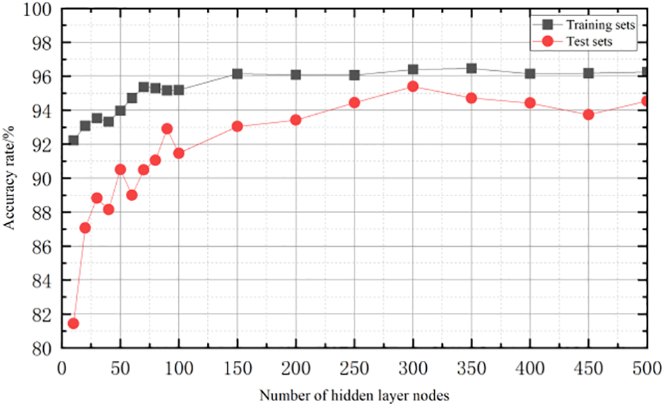
Figure 10: Optimum of hidden layer nodes of ELM

The proposed five accuracy indexes (including AR, RR, SR, MDR, and FAR) are used to comprehensively evaluate the accuracy of the classifiers. If the accuracy of SVM and ELM does not meet the requirements, it is necessary to reset the parameters, train, and test.

After the prediction results in Z1 of SVM and Z2 of ELM are obtained, the credibility of the prediction results made by the two data-driven methods is evaluated by introducing the Sigmoid function, and the credibility index R1 of SVM and the credibility index R2 of ELM are obtained respectively. To illustrate the relationship between the credibility and accuracy of SVM and ELM, the relationship curve between them can be given by setting different credibility thresholds, as shown in Fig. 11.

Figure 11: Relation between credibility and accuracy

5.2 Performance of Model-Driven Method

The model-driven time domain simulation method, energy function method and, RCKE method are used to assess the transient stability of the New England system, respectively. It is necessary to elaborate the steps of the standard energy function method first. Since the classical model of a multi-machine power system has been given in Eqs. (1)~(4), where Eq. (4) represents the kinetic energy of the ith generator, the transient energy function of the system at any time can be expressed as

V=12∑i=1nMiωi2+∑i=1n∫δ0iδi(PeiIII−Pmi)dδi(31)

where the first part corresponds to the kinetic energy of the system and the second part corresponds to the potential energy of the system; δ0i is the reference point of potential energy; PeiIII  corresponds to the electromagnetic power of the ith generator after the fault is cleared. Thus, the steps of the energy function method are as below: firstly, substitute the unstable equilibrium point, i.e., (δu,0), into Eq. (31) and obtain the critical energy of the system Vcr; secondly, substitute the state of the system when the fault is cleared, i.e., (δcl,ωcl), into Eq. (31) and obtain the energy of the system when the fault is cleared Vcl; finally, Vcr>Vcl indicates the system is stable while Vcr≤Vcl indicates the system is unstable.

The transient stability results and calculation time of these three methods are shown in Figs. 12 and 13, respectively. Among them, the fault locations are 2*–3 (indicating that a three-phase short-circuit fault occurred on bus 2, and the system cuts off 2–3 lines after the fault), 4*–14, 6*–11, 15*–16, 24*–23, and 25*–26.

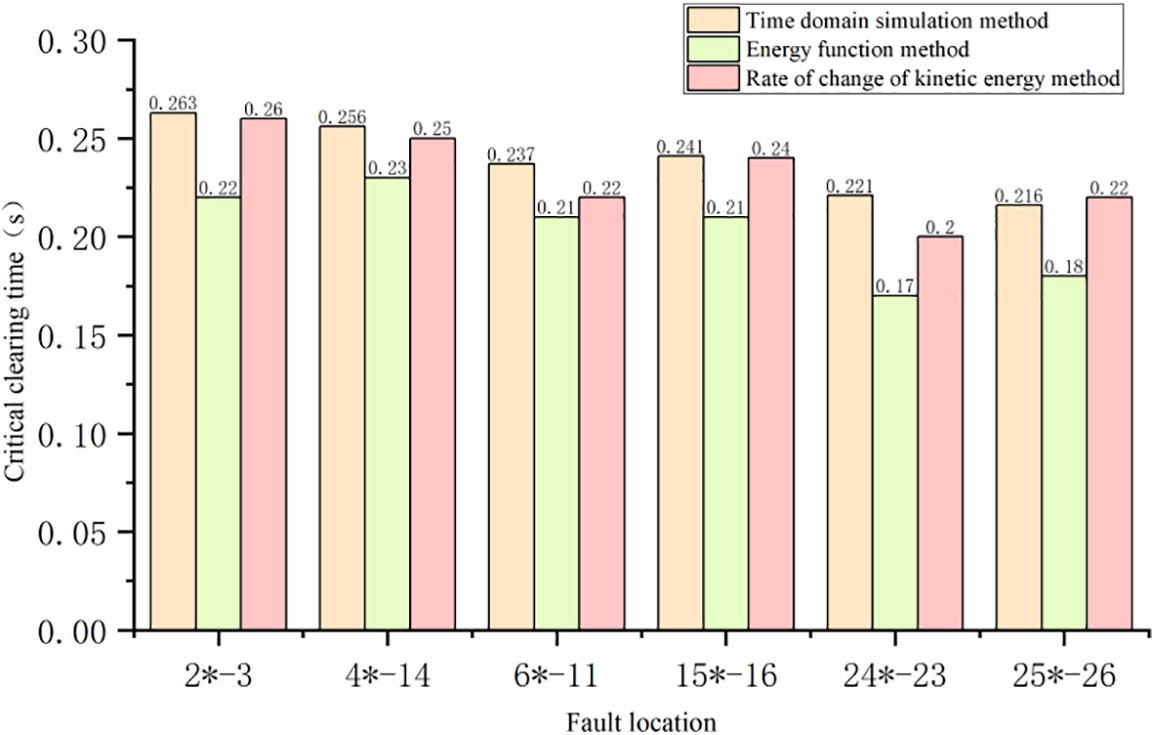
Figure 12: Transient stability assessment results of model-driven methods

Figure 13: Computation time of model-driven methods

It can be seen that, on the one hand, although both the energy function method and the RCKE method belong to the direct methods, the accuracy of the assessment result of the latter method is relatively higher, because the Lyapunov function constructed by the energy function method is usually more conservative than the actual system. On the other hand, when applied to the online assessment of transient stability of multi-machine power systems, the RCKE method is more efficient than the energy function method because it adopts the piecewise solution methods, and the calculation efficiency of the time domain simulation method is not suitable for online because it needs the integral solution of the whole process.

5.3 Performance of Proposed Parallel Integrated Model-Driven and Data-Driven Method

The Monte Carlo method mentioned above is used to generate a sample data set containing 1000 samples, which is used to test the performance of the proposed parallel integrated model-driven and data-driven method and to show the average accuracy and average calculation time of its transient stability assessment.

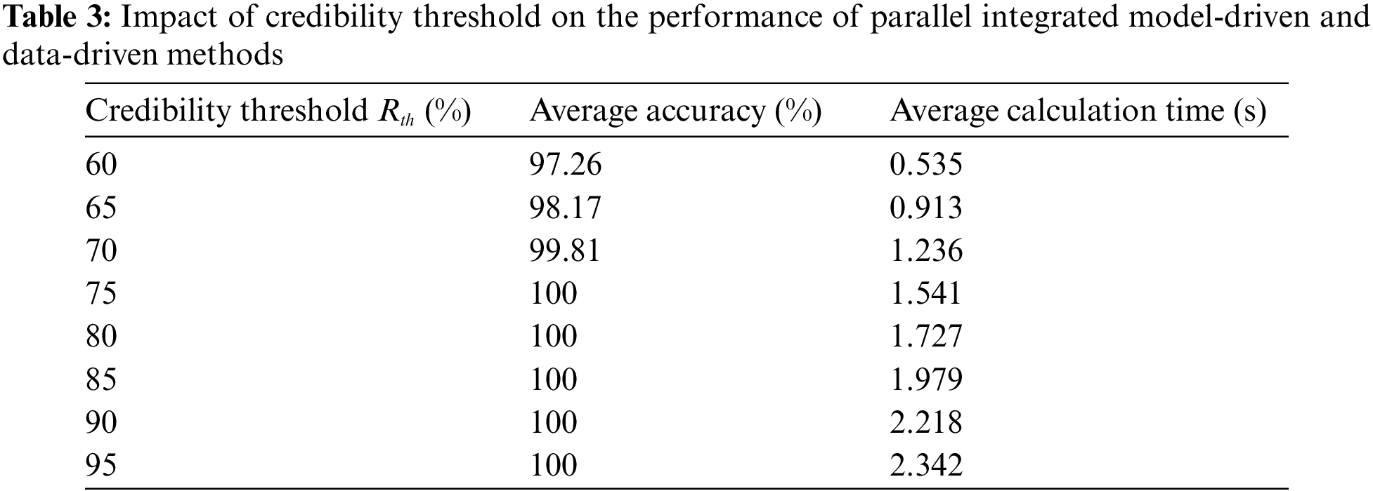
As shown in Section 4.5, there is only one hyperparameter in the proposed method: the credibility threshold Rth. In essence, Rth represents the respective contributions of the model-driven method and data-driven method, and it is a central element in determining the performance of the proposed method because it controls how frequently the model-driven method needs to be activated. Based on the relation between the accuracy and credibility of a single classifier which is discussed in Section 4.3, a reasonable value of Rth seems to be about 90%. However, note that both the SVM classifier and ELM classifier are used in the data-driven stage and that the switching function is established according to the independence of these two classifiers, therefore, Rth should be determined by data experiment. In summary, as for the performance of the proposed parallel integrated method, a larger Rth represents the preference for credibility, while a smaller Rth represents the preference of efficiency.

The influence of the credibility threshold on the assessment performance of the proposed method is shown in Table 3. It can be seen that with the gradual increase of the credibility threshold, on the one hand, the average calculation time of the proposed method will be longer and longer, because the higher credibility threshold means that the RCKE method needs to be activated more frequently for transient stability assessment. On the other hand, the average accuracy of the proposed method will increase continuously, and when the credibility threshold increases to 75%, the average accuracy will reach 100%, which will remain unchanged thereafter. Therefore, considering the factors of assessment accuracy and calculation time, this paper sets the credibility threshold as 80%.

Similarly, the sample data set with 1000 samples generated above is used to test the transient stability assessment performance of the energy function method, support vector machine, and extreme learning machine, and the results are shown in Fig. 14. It should be pointed out that Fig. 14 is a double Y-axis diagram, where the left Y-axis represents the average computation time while the right Y-axis represents the average accuracy rate. It can be seen that the computational efficiency of the proposed method is greatly improved compared with the energy function method. On the other hand, compared with the traditional single data-driven methods (such as support vector machine and extreme learning machine), the proposed method has higher assessment accuracy. Furthermore, the proposed method actually provides a route to adjust its credibility level (i.e., credibility threshold Rth and switching function), and under extreme conditions (e.g., the quality of the input data set is too low) the proposed method can totally degenerate into the model-driven RCKE method which represents a 100% credibility level, while the credibility of SVM and ELM classifiers is inherent which means their output results always have some inevitable uncertainties. Therefore, the proposed method has higher credibility than SVM and ELM, through Table 3 and Fig. 14.

Figure 14: Comparison of transient stability assessment results of different methods

For the actual power system, the measurement data obtained from the SCADA system often contain noise, which will affect the accuracy of transient stability assessment results by data-driven methods. In order to simulate a real scene, random variables that follow normal distribution are added to the original feature set as irrelevant features in the sample data generation stage. The influence of the number of irrelevant features on the average accuracy of transient stability assessment by different methods is shown in Fig. 15. It can be seen that with the increasing number of irrelevant features, the average accuracy of single data-driven methods (such as support vector machines and extreme learning machines) will gradually decrease, while the average accuracy of the proposed method will remain unchanged, which indicates that the proposed method of this paper has a better anti-noise ability.

Figure 15: Impact of the irrelevant feature on mean accuracy

6  Conclusions

In this paper, a new two-stage parallel integrated model-driven and data-driven online transient stability assessment method is proposed, which has advantages over the traditional single-type driven methods, and the following conclusions are obtained:

(1)   In the data-driven stage, support vector machine classifiers, and extreme learning machine classifiers with different internal principles are used to predict the transient stability, thus ensuring the independence of each other.

(2)   The output results of data-driven methods depend on the input sample data and offline training parameters, so they have some uncertainties. Based on the distance between the output results and the classification critical points, the credibility index of data-driven methods is proposed to quantify the credibility level of their transient stability assessment.

(3)   A switching function based on the established credibility index is proposed, and whether the model-driven rate of change of the kinetic energy method is activated or not is decided by the switching function. Thus, the model-driven method and the data-driven methods are combined by a “parallel integrated” pattern through the switching function. Compared with the single data-driven method, the proposed method can obtain more reliable transient stability assessment results (i.e., higher credibility level and stronger anti-noise ability) on the premise of ensuring the calculation efficiency.

(4)   This paper assumes that each synchronous generator of a multi-machine power system is represented by the second-order classical model. However, nowadays fast controllers (e.g., automatic voltage regulators, and governors) are equipped in practical power systems, and the proposed method in this paper cannot cope with this complicated situation. In our future research, the RCKE method in the model-driven stage should be replaced by a more powerful method such as the recursive approach based on corrected kinetic energy which was proposed in reference [6], while the input features in the data-driven stage should include details of practical synchronous generators and corresponding fast controllers.

Acknowledgement: We would like to thank the reviewers and the editor for their valuable comments and suggestions.

Funding Statement: This research was funded by the Science and Technology Project of State Grid Shanxi Electric Power Co., Ltd. (Project No. 520530200013).

Author Contributions: The authors confirm contribution to the paper as follows: study conception and design: Ying Zhang, Xiaoqing Han and Gengwu Zhang; data collection: Chao Zhang, Ying Qu and Yang Liu; analysis and interpretation of results: Ying Zhang and Ying Qu; draft manuscript preparation: Ying Zhang, Chao Zhang and Ying Qu. All authors reviewed the results and approved the final version of the manuscript.

Availability of Data and Materials: The data that support the findings of this study are available on request from the authors, upon reasonable request.

Conflicts of Interest: The authors declare that they have no conflicts of interest to report regarding the present study.

References

1. Tang, C. K., Graham, C. E., El-Kady, M., Alden, R. T. H. (1994). Transient stability index from conventional time domain simulation. IEEE Transactions on Power Systems, 9(3), 1524–1530. [Google Scholar]

2. Narasimhamurthi, N., Musavi, M. (1984). A generalized energy function for transient stability analysis of power systems. IEEE Transactions on Circuits and Systems, 31(7), 637–645. [Google Scholar]

3. Llamas, A., Lopez, J. D. L. R., Mili, L., Phadke, A. G., Thorp, J. S. (1995). Clarifications of the BCU method for transient stability analysis. IEEE Transactions on Power Systems, 10(1), 210–219. [Google Scholar]

4. Xue, Y., van Custem, T., Ribbens-Pavella, M. (1989). Extended equal area criterion justifications, generalizations, applications. IEEE Transactions on Power Systems, 4(1), 44–52. [Google Scholar]

5. Al-Taee, A. A., Al-Taee, M. A., Al-Nuaimy, W. (2016). Augmentation of transient stability margin based on rapid assessment of rate of change of kinetic energy. Electric Power Systems Research, 140(2), 588–596. [Google Scholar]

6. Jahromi, M. Z., Kouhsari, S. M. (2016). A novel recursive approach for real-time transient stability assessment based on corrected kinetic energy. Applied Soft Computing, 48(5), 660–671. [Google Scholar]

7. Hu, W., Lu, Z., Wu, S., Zhang, W., Dong, Y. et al. (2019). Real-time transient stability assessment in power system based on improved SVM. Journal of Modern Power Systems and Clean Energy, 7(1), 26–37. [Google Scholar]

8. Shahzad, U. (2022). A comparative analysis of artificial neural network and support vector machine for online transient stability prediction considering uncertainties. Australian Journal of Electrical and Electronics Engineering, 19(2), 101–116. [Google Scholar]

9. Tian, F., Zhou, X., Yu, Z., Shi, D., Chen, Y. et al. (2019). A preventive transient stability control method based on support vector machine. Electric Power Systems Research, 170(3), 286–293. [Google Scholar]

10. Kim, H., Singh, C. (2005). Power system probabilistic security assessment using Bayes classifier. Electric Power Systems Research, 74(1), 157–165. [Google Scholar]

11. Guo, T., Milanović, J. V. (2013). Probabilistic framework for assessing the accuracy of data mining tool for online prediction of transient stability. IEEE Transactions on Power Systems, 29(1), 377–385. [Google Scholar]

12. Behdadnia, T., Yaslan, Y., Genc, I. (2021). A new method of decision tree based transient stability assessment using hybrid simulation for real-time PMU measurements. IET Generation, Transmission & Distribution, 15(4), 678–693. [Google Scholar]

13. Zhang, C., Li, Y., Yu, Z., Tian, F. (2016). Feature selection of power system transient stability assessment based on random forest and recursive feature elimination. 2016 IEEE PES Asia-Pacific Power and Energy Engineering Conference, pp. 1264–1268. Xi’an, China. [Google Scholar]

14. Chen, Y., Mazhari, S. M., Chung, C. Y., Faried, S. O., Wang, B. et al. (2019). Power system on-line transient stability prediction by margin indices and random forests. 2019 IEEE Electrical Power and Energy Conference, pp. 1–6. Montreal, Canada. [Google Scholar]

15. Li, X., Liu, C., Guo, P., Liu, S., Ning, J. (2022). Deep learning-based transient stability assessment framework for large-scale modern power system. International Journal of Electrical Power & Energy Systems, 139(6), 108010. [Google Scholar]

16. Ren, C., Xu, Y., Zhang, R. (2021). An interpretable deep learning for power system transient stability assessment via tree regularization. IEEE Transactions on Power Systems, 37(5), 3359–3369. [Google Scholar]

17. Zhu, L., Hill, D. J., Lu, C. (2019). Hierarchical deep learning machine for power system online transient stability prediction. IEEE Transactions on Power Systems, 35(3), 2399–2411. [Google Scholar]

18. Ren, C., Xu, Y., Zhang, R. (2022). An Interpretable deep learning method for power system transient stability assessment via tree regularization. IEEE Transactions on Power Systems, 37(5), 3359–3369. [Google Scholar]

19. Zhao, T., Wang, J., Lu, X., Du, Y. (2021). Neural lyapunov control for power system transient stability: A deep learning-based approach. IEEE Transactions on Power Systems, 37(2), 955–966. [Google Scholar]

20. Azman, S. K., Isbeih, Y. J., El Moursi, M. S., Elbassioni, K. (2020). A unified online deep learning prediction model for small signal and transient stability. IEEE Transactions on Power Systems, 35(6), 4585–4598. [Google Scholar]

21. Li, Y., Yang, Z. (2017). Application of EOS-ELM with binary Jaya-based feature selection to real-time transient stability assessment using PMU data. IEEE Access, 5, 23092–23101. [Google Scholar]

22. Zhang, Y., Zhao, Q., Tan, B., Yang, J. (2021). A power system transient stability assessment method based on active learning. The Journal of Engineering, 2021(11), 715–723. [Google Scholar]

23. Wang, H., Wang, Q., Chen, Q. (2020). Transient stability assessment model with improved cost-sensitive method based on the fault severity. IET Generation, Transmission & Distribution, 14(20), 4605–4611. [Google Scholar]

24. Li, F., Wang, Q., Tang, Y., Xu, Y., Dang, J. (2021). Hybrid analytical and data-driven modeling based instance-transfer method for power system online transient stability assessment. CSEE Journal of Power and Energy Systems, 1–10. https://ieeexplore.ieee.org/abstract/document/9420351 [Google Scholar]

25. Li, F., Wang, Q., Tang, Y., Xu, Y. (2021). An integrated method for critical clearing time prediction based on a model-driven and ensemble cost-sensitive data-driven scheme. International Journal of Electrical Power & Energy Systems, 125(11), 106513. [Google Scholar]

26. Ai-Taee, M. A., Ai-Azzawi, F. J., Al-Taee, A. A., Al-Jumaily, T. Z. (2001). Real-time assessment of power system transient stability using rate of change of kinetic energy method. IEEE Proceedings-Generation, Transmission and Distribution, 148(6), 505–510. [Google Scholar]

27. Johnson, C. R. (1990). Matrix theory and applications, vol. 40. USA: American Mathematical Society Press. [Google Scholar]

28. Müller, K. R., Mika, S., Tsuda, K., Schölkopf, K. (2018). An introduction to kernel-based learning algorithms. In: Handbook of neural network signal processing, pp. 4–10. USA: CRC Press. [Google Scholar]

29. Zhang, Y., Xu, Y., Dong, Z. Y., Xu, Z., Wong, K. P. (2017). Intelligent early warning of power system dynamic insecurity risk: Toward optimal accuracy-earliness tradeoff. IEEE Transactions on Industrial Informatics, 13(5), 2544–2554. [Google Scholar]