
 Submit a Paper
 Propose a Special lssue
 Open Access
ARTICLE

The Non-Singular Fast Terminal Sliding Mode Control of Interior Permanent Magnet Synchronous Motor Based on Deep Flux Weakening Switching Point Tracking
College of Electrical and Information Engineering, Hunan University of Technology, Zhuzhou, 412007, China
* Corresponding Author: Kaihui Zhao. Email:
Energy Engineering 2023, 120(2), 277-297. https://doi.org/10.32604/ee.2023.022461
Received 10 March 2022; Accepted 27 May 2022; Issue published 29 November 2022
 View Full Text
 Download PDF
Abstract
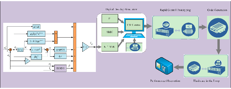
This paper presents a novel non-singular fast terminal sliding mode control (NFTSMC) based on the deep flux weakening switching point tracking method in order to improve the control performance of permanent interior magnet synchronous motor (IPMSM) drive systems. The mathematical model of flux weakening (FW) control is established, and the deep flux weakening switching point is calculated accurately by analyzing the relationship between the torque curve and voltage decline curve. Next, a second-order NFTSMC is designed for the speed loop controller to ensure that the system converges to the equilibrium state in finite time. Then, an extended sliding mode disturbance observer (ESMDO) is designed to estimate the uncertainty of the system. Finally, compared with both the PI control and sliding mode control (SMC) by simulations and experiments with different working conditions, the method proposed has the merits of accelerating convergence, improving steady-state accuracy, and minimizing the current and torque pulsation.Graphic Abstract
Keywords
Interior permanent magnet synchronous motor (IPMSM) has merits concering simple structure, flux density and strong coercivity of neodymium-iron-boron permanent magnet [1]. IPMSM has a stronger load-carrying capacity than surface-mounted permanent magnet synchronous motor (SPMSM) because of the uneven air gap field distribution [2]. In addition, a wider speed range can be obtained by adopting the flux weakening (FW) control strategy. Thus, IPMSM is widely used in engineering fields such as aerospace, rail transit, and intelligent robots [3].
Common FW control strategies include the formula calculation method, lookup table (LUT), gradient descent, and negative d-axis current compensation [4]. The formula calculation method [5] is highly dependent on the motor parameters, and the control performance of the system decline in the case of system disturbance, such as parameter perturbation. The LUT method [6] completely depends on a large amount of experimental data, and it is not universally applicable for motors with different types and parameters. The current gradient descent method [7] analyzes the relationships between torque change direction and the position relation of limited voltage circle to correct the current of the d-q axis. However, the steps of calculation are complicated and tedious. The negative d-axis current compensation method [8,9] is simple, and the control system has better robustness because it does not depend on the motor parameters. When the voltage inverter is saturated, FW control is completed by applying compensation to the d-axis current.
At present, the PI algorithm has become the mainstream method for FW control because of its simple algorithms and mature technology. The PI algorithm is a linear control method that is widely used in motor control. However, IPMSM is a nonlinear system with various uncertainties, such as internal disturbance caused by high-speed and unmodeled dynamic excitation caused by deepened coupling of the d-q current regulator, which may affect the control performance of the system [10]. Eliminating PI control disturbances is difficult to due to its limitations, such as integral saturation, which is unsuitable for applying high-performance occasions [11].
Many advanced nonlinear control theories have been applied in IPMSM high-performance in recent years. For example, model predictive control (MPC) [12], optimize feedforward control [13], neural network control [14], and so on. A single MPC controller with a brand-new linearization method was designed to tackle the strong coupled nonlinear IPMSM mathematical model [12]. A novel modification of the optimal torque control for IPMSM was adopted to optimize the control performance with time-varying parameters [13]. A feedforward neural network controller was adopted to solve the finite control set model predictive control (FCS-MPC) [14]. To some extent, the above control algorithms [12–14] depend on the known mathematical model and the system’s nominal model and can be considered model-based control theory. However, IPMSM is a complex, nonlinear and time-varying system that has unavoidable parameter perturbations that are difficult to be modeled and measured. Thus, the above algorithms have some limitations in engineering applications.
To reduce the dependence on motor parameters, sliding mode control (SMC) has become a hot topic vis-a-vis the FW control of IPMSM. An SMC controller was designed to replace the PI controller in the voltage closed-loop [15], which accelerates the dynamic adjustment rate when the voltage inverter is saturated and enhances the anti-disturbance ability of the control system. An SMC controller based on the anti-integral saturation regulator [16,17] not only enhances the system’s robustness, but also improves the current tracking performance and inhibits the torque ripple. The SMC speed controller based on the new sliding mode reaching law [18,19] was adopted to optimize the sliding mode switching performance, weaken chattering and improve the control performance of the system. However, for conventional SMC, the convergence of the system error is exponential asymptotic, and it cannot converge to zero in finite time. Therefore, the key technologies in FW control research are how accelerating the convergence of speed, improve the steady-state control accuracy, and enhance the disturbance resistance of the control system.
This paper presents a novel NFTSMC method based on deep flux weakening switching point tracking. It achieves fast and accurate tracking of reference speed and improves the robustness of the IPMSM drive system. The main contributions of this paper are summarized as follows:
i) This method that combines NFTSMC with FW control is presented to improve the speed response of the IPMSM in flux weakening region. It has the features of both NFTSMC and FW control. More specifically, while the FW control based on deep flux weakening switching point tracking expands the actual speed range, the NFTSMC based on extended sliding mode disturbance observer (ESMDO) accelerates speed convergence, improves steady-state accuracy, and minimizes the current pulsation and torque pulsation.
ii) The mathematical model of MTPV control is simplified. The deep flux weakening switching point is obtained by analyzing the relationship between the torque and the voltage drop curves.
iii) The NFTSMC speed controller is designed based on the input and the output, which reduces the dependence on motor parameters.
iv) ESMDO estimates the unknown part of external disturbances. It is added to the input of the NFTSMC speed controller as a feedforward compensation item.
Ignoring stator core saturation, eddy current, and hysteresis loss, permanent rotor magnet without winding damping winding and mutual leakage inductance between stator windings, stator voltage equation of IPMSM in the d-q reference can be described as [20]:
where
In steady-state operation, the stator voltages can be approximately simplified as:
The motor operation should meet the following requirements:
where
FW control consists of three processes: maximum torque per ampere (MTPA) control, constant power control, and maximum torque per volt (MTPV) control.
Fig. 1 presents the d-q-axis current trajectory diagram of FW control.
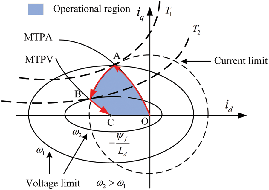
Figure 1: The d-q-axis current trajectory diagram of FW control
2.1 Maximum Torque Per Ampere (MTPA) Control
When the actual motor speed is lower than the nominal speed, the current trajectory of MTPA runs along the curve OA in Fig. 1. The electromagnetic torque remains constant during motor acceleration. In the d-q reference, the equations of electromagnetic torque and stator current are [21]:
Constructing Lagrange function from Eq. (4), the stator current of d-q axis can be obtained as [22]:
where
2.2 Maximum Torque Per Volt (MTPV) Control
The current trajectory in the shallow flux weakening region runs along with the curve AB in Fig. 1. The motor’s actual speed is higher than the nominal speed, and the method of adding a negative d-axis current should be adopted to avoid saturation of the voltage inverter.
The current trajectory in the deep flux weakening region runs along the curve BC in Fig. 1. The MTPV control is suitable for the motor, which meets the requirement of
Substituting Eqs. (2)–(4) into Eq. (6) yields
The expression of the d-axis current can be obtained as:
3 Optimization of Deep Flux Weakening Control
3.1 Negative D-Axis Current Compensated Method
When the motor is running, the saturation of the output voltage of the inverter is judged by constructing a voltage closed-loop. When
where
3.2 The Principle of Determination of Deep Flux Weakening Switching Point
The conventional d-axis negative compensation method usually sets point E (
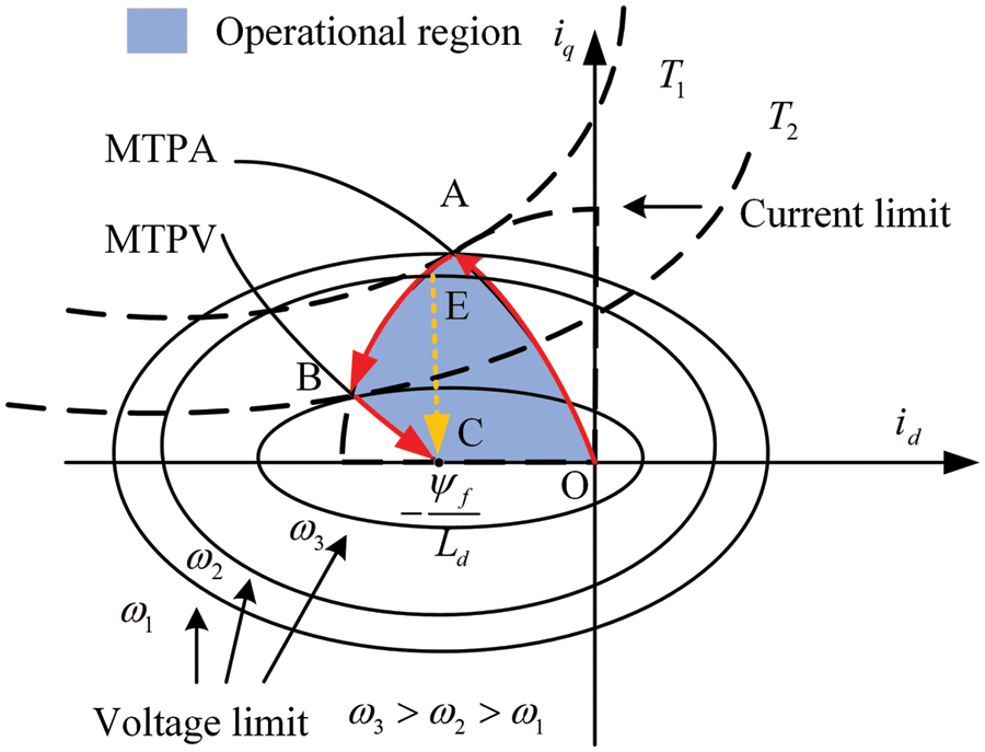
Figure 2: The d-q axis current trajectory diagram of negative d-axis current compensation
The current trajectory moves leftward from point A to point B. If setting point E as a switching point, the actual current cannot reach point B, resulting in a narrow speed regulation range. It can be seen from Fig. 2 that, in order to reach point B and expand the speed regulation range, the torque curve at point B is tangent to the limited voltage. From Eq. (2),
According to Eq. (4), the direction of torque change is written in matrix form
Substituting Eq. (2) into Eq. (3) yields
To obtain the decline direction of voltage, a new voltage change function is designed by
Combining Eqs. (2) and (12), the direction of voltages decline is written as a form of matrix
According to Eqs. (10) and (13), the switching signal is constructed as:
where
The q-axis current can be designed as
To further simplify the control algorithm, the relationship between compensation value of q-axis current and
where
where
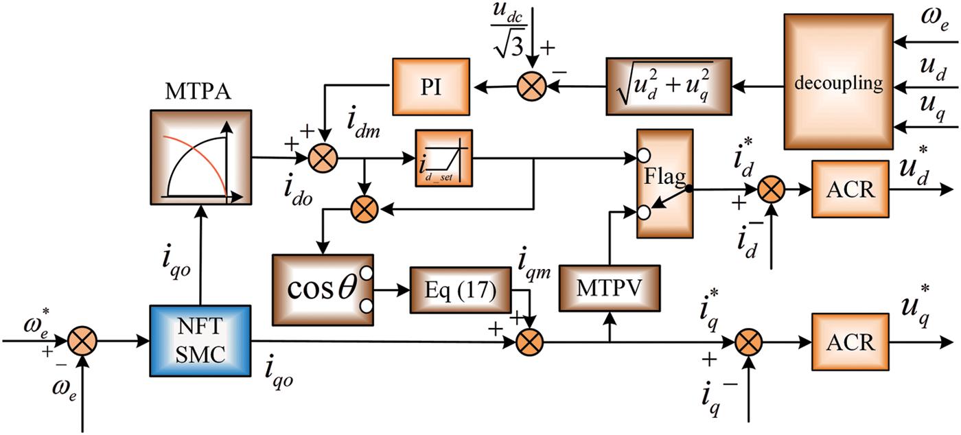
Figure 3: The block diagram of FW control
To avoid integral saturation of PI and chattering problem of SMC, a second-order NFTSMC speed controller is designed to improve the performance of IPMSM, and an ESMDO is designed to estimate the unknown disturbances.
4.1 Designed of NFTSMC Speed Control
The equation of electromagnetic torque Eq. (4) can be described as:
where
The mechanical motion equation of IPMSM is:
Substituting Eq. (19) into Eq. (20) yields
where
To accelerate speed transient response and improve steady-state control accuracy, an NFTSMC speed controller is designed. From Eq. (21), the control law of speed controller can be designed as:
where
Substituting Eq. (21) into Eq. (22) yields
Define the state error of the controller as:
Then, the state variable is defined as
Selecting a second-order NFTSMC surface as below [26]:
where
Choose the exponential reaching law as:
where
Theorem 1: For the rotational speed error Eq. (24), chosen Eq. (25) as the sliding mode surface and Eq. (27) as reaching law, then the system state will converge to zero in finite time.
From Eqs. (26) and (27), the feedback control law of the NFTSMC is obtained as below:
Proof: Selecting Lyapunov function candidate to be
The derivative of V is:
Due to
It completes the proof.
Substituting Eq. (28) into Eq. (22), we can obtain the total control law
Fig. 4 presents the schematic diagram of the NFTSMC speed controller.
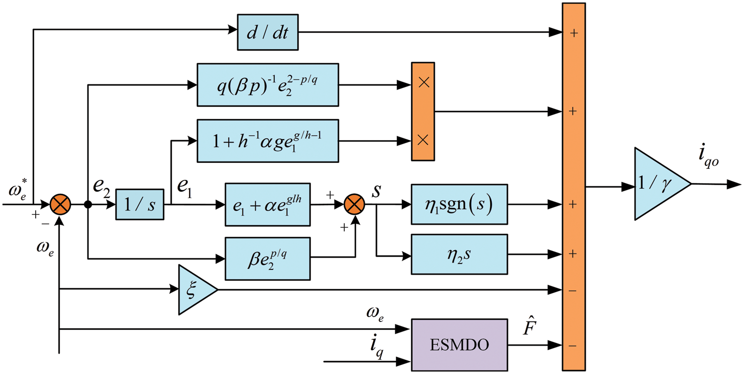
Figure 4: The schematic diagram of NFTSMC speed controller
4.2 Extended Sliding Mode Disturbance Observer
The ESMDO can estimate the uncertainty of the system by measuring the input and output of the actual system. It provides not only practical feasibility for the technical realization and practical applications in motor control. The variable is defined as
where
Combining Eqs. (21) and (32) obtains the equation:
where
Select the speed error as the sliding mode surface:
Choose the exponential reaching law as:
where
The control law of the sliding mode observer can be obtained from Eqs. (33) to (35):
Theorem 2: The error
Proof: Selecting Lyapunov function candidate to be:
The derivative of
Chosen
It completes the proof.
Substituting Eq. (36) into Eq. (32), the total disturbance estimation expression is:
Substituting Eq. (39) into Eq. (31) yields
To weaken the chattering of the system due to the sgn function, the continuous saturation function
where
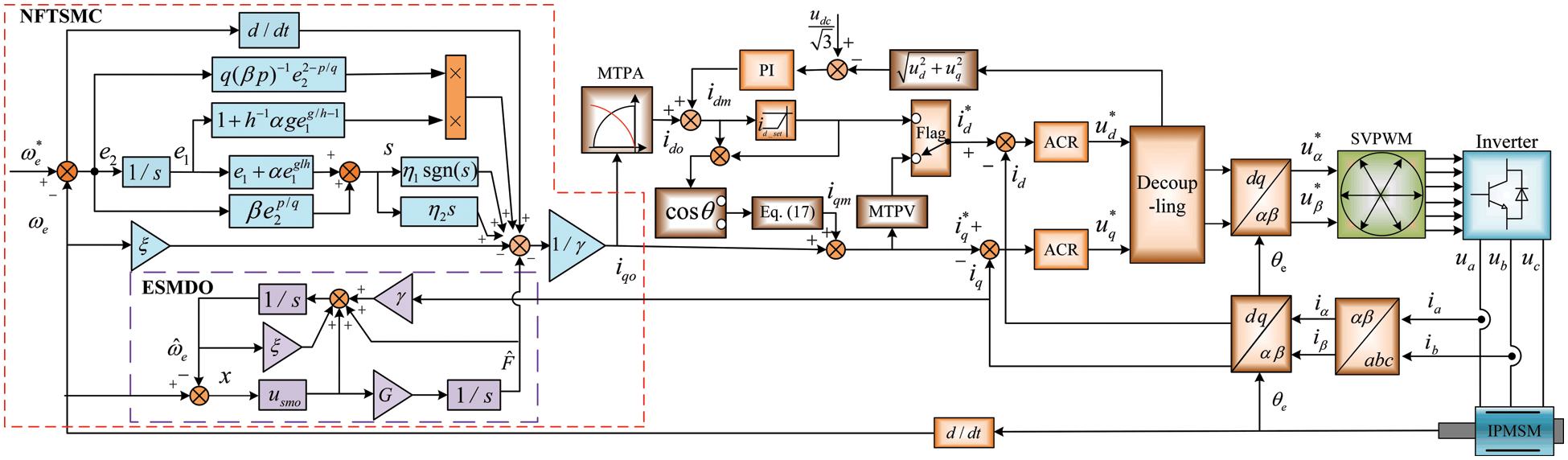
Figure 5: The block diagram of IPMSM drive system
To verify the feasibility and effectiveness of the proposed method, this section demonstrates the comparative analysis results of simulations and experiments.
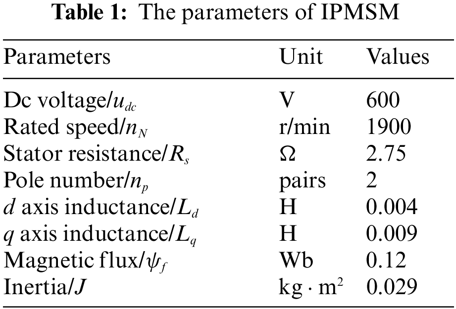
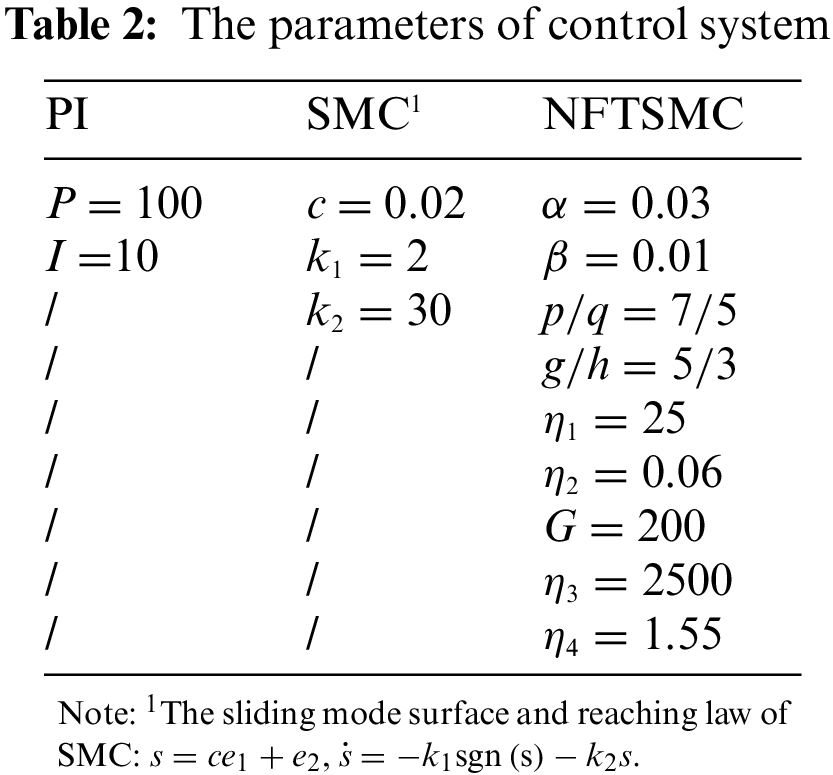
MATLAB/Simulink simulation is used to build a motor model compared with PI, conventional SMC, and NFTSMC. Table 1 represents the parameters of IPMSM. The drive system parameters of PI, SMC and NFTSMC are listed in Table 2.
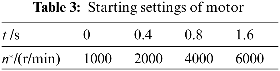
Case 1: Graded speed regulation condition
The load torque is set as
Figs. 6a–6c demonstrate the simulation comparison results of speed, torque, and d-q axis current controlled by PI, SMC, and NFTSMC; Figs. 6d and 6e show the observed value of
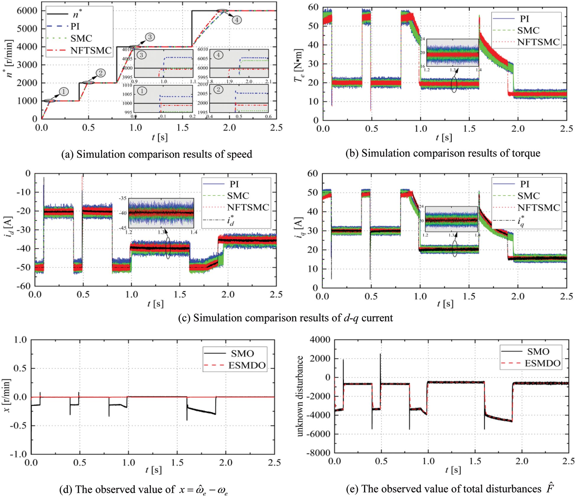
Figure 6: Simulation results of PI/SMC/ NFTSMC with graded speed regulation condition
The simulation comparison results are summarized in Table 4. For intuitive comparison, the comparison data of Table 4 is graphically processed to obtain Fig. 7.
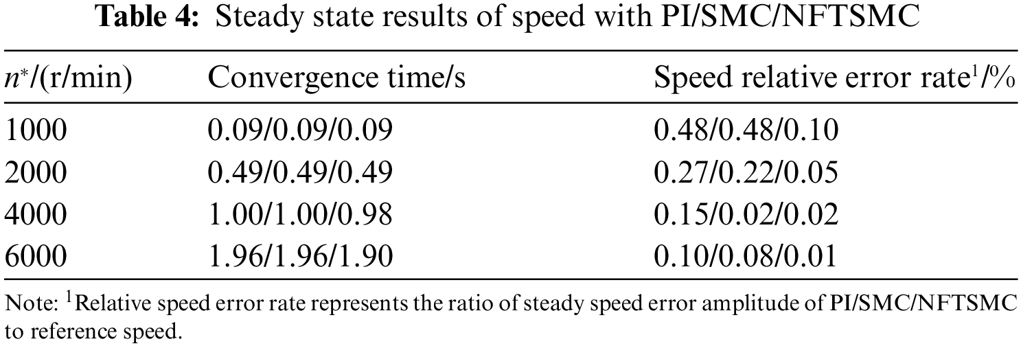
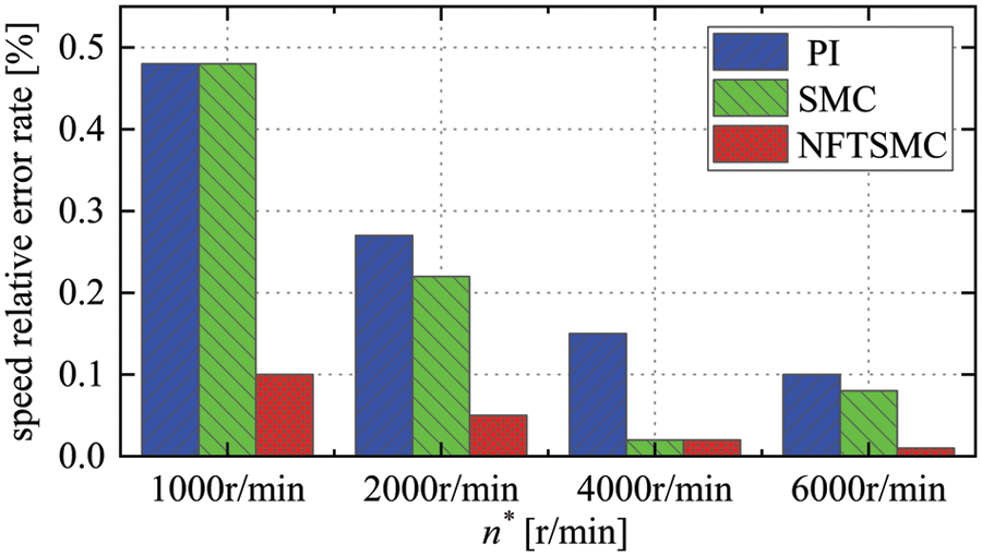
Figure 7: The comparison of speed relative error rate
From Figs. 6a and 7, and Table 4, NFTSMC has better steady-state control accuracy than PI and SMC. When the reference speed changes from 2000 to 4000 r/min at 0.8 s, NFTSMC takes 0.18 s to reach steady-state, and the relative error rate of speed is only 0.02%. PI and SMC take 0.20 s to reach steady-state, and the relative error rate of speed are 0.15% and 0.02%. NFTSMC improves the dynamic response rate by 10%. When the reference speed changes from 4000 to 6000 r/min at 1.2 s, NFTSMC takes 0.3 s to reach reference speed, and the relative error rate of speed is only 0.01%. PI and SMC take 0.36 s to reach steady-state, and the relative error rate of speed is 0.10% and 0.08%. NFTSMC improves the dynamic response rate by 8%. In general, the NFTSMC speed controller can accelerate the dynamic convergence of speed in the flux weakening regions and further minimize the steady-state error of speed.
Figs. 6b and 6c demonstrate that the torque and d-q axis current waveform of NFTSMC are more stable, with smaller pulsation and better transient stability performance of the motor. It further shows that NFTSMC can effectively improve the control performance of the motor drive system.
Figs. 6d and 6e demonstrate that the unknown disturbance and the speed observed by ESMDO is more accurate than that observed by SMO. This shows that the performance of ESMDO is better than SMO.
Case 2: Uniform acceleration condition
Setting the reference speed as a slope function to simulate uniform acceleration condition. Figs. 8a–8c demonstrate the simulation comparison of speed, torque, and d-q axis current controlled by PI, SMC, and NFTSMC; Figs. 8d and 8e show the observed value of
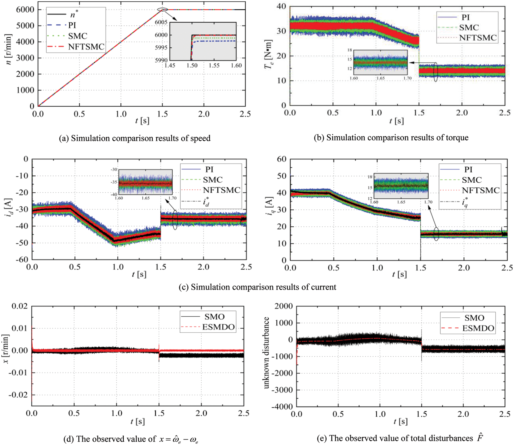
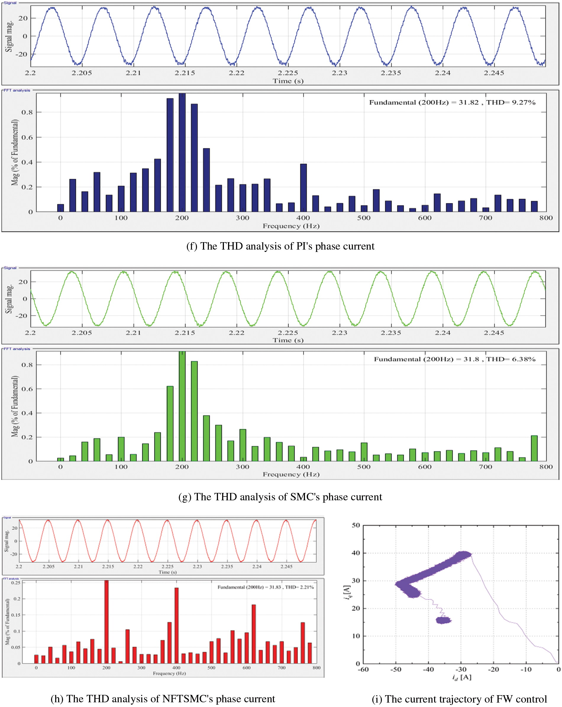
Figure 8: Simulation results of PI/SMC/NFTSMC with uniform acceleration condition
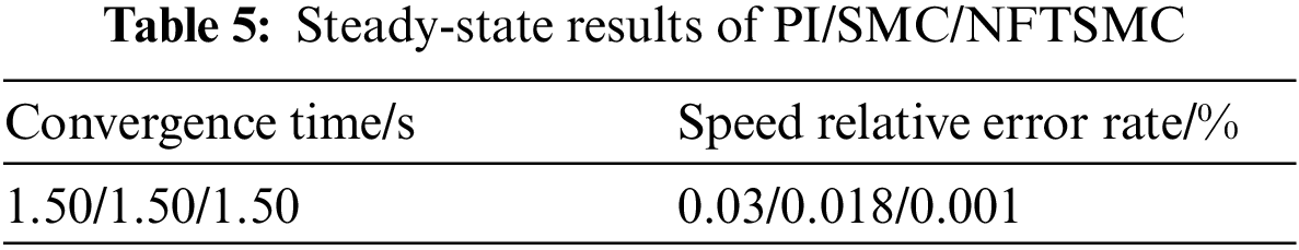
From Fig. 8a and Table 5, there is no significant difference in the speed response rate of three methods with uniform acceleration, but the control accuracy of NFTSMC is significantly better than PI and SMC. Combined with Figs. 8a, 8d, and 8e, the unknown disturbances are estimated quickly by ESMDO to ensure that NFTSMC can effectively reduce chattering and improve the robustness of the drive system.
Figs. 8b and 8c demonstrate that the torque and current pulsation of PI are the largest and the convergence performance is the worst in the motor operation process. NFTSMC has the most stable d-q axis current and torque, and the pulsation of NFTSMC is the smallest. The simulation results show that the NFTSMC speed controller performs better transient steady-state control.
Fig. 8i demonstrates the current track diagram of NFTSMC. It is shown that the simulation current track conforms to the theoretical track of FW control. The d-axis current value of the deep flux weakening switching point is about –48A, far greater than the value of conventional settings, which verifies the correctness and effectiveness of the proposed method.
From Figs. 8f–8h, the THD value of phase current for PI is about 9.27%, and the THD value of phase current for SMC is about 6.38%. The THD value of phase current for NFTSMC is only 2.21%. The phase current of NFTSMC is much smoother. It means that the current harmonics of NFTSMC are smaller than PIs and SMCs. The comparison of THD analysis for phase current indicates that the drive system of NFTSMC has better control performance.
To further test the effectiveness of the proposed method, the hardware-in-the-loop simulation (HILS) of IPMSM is carried out with DSP-TMS320F2812 and RT-Lab (OP5600) HILS platform. Fig. 9 shows the configuration diagram for the IPMSM drive systems.
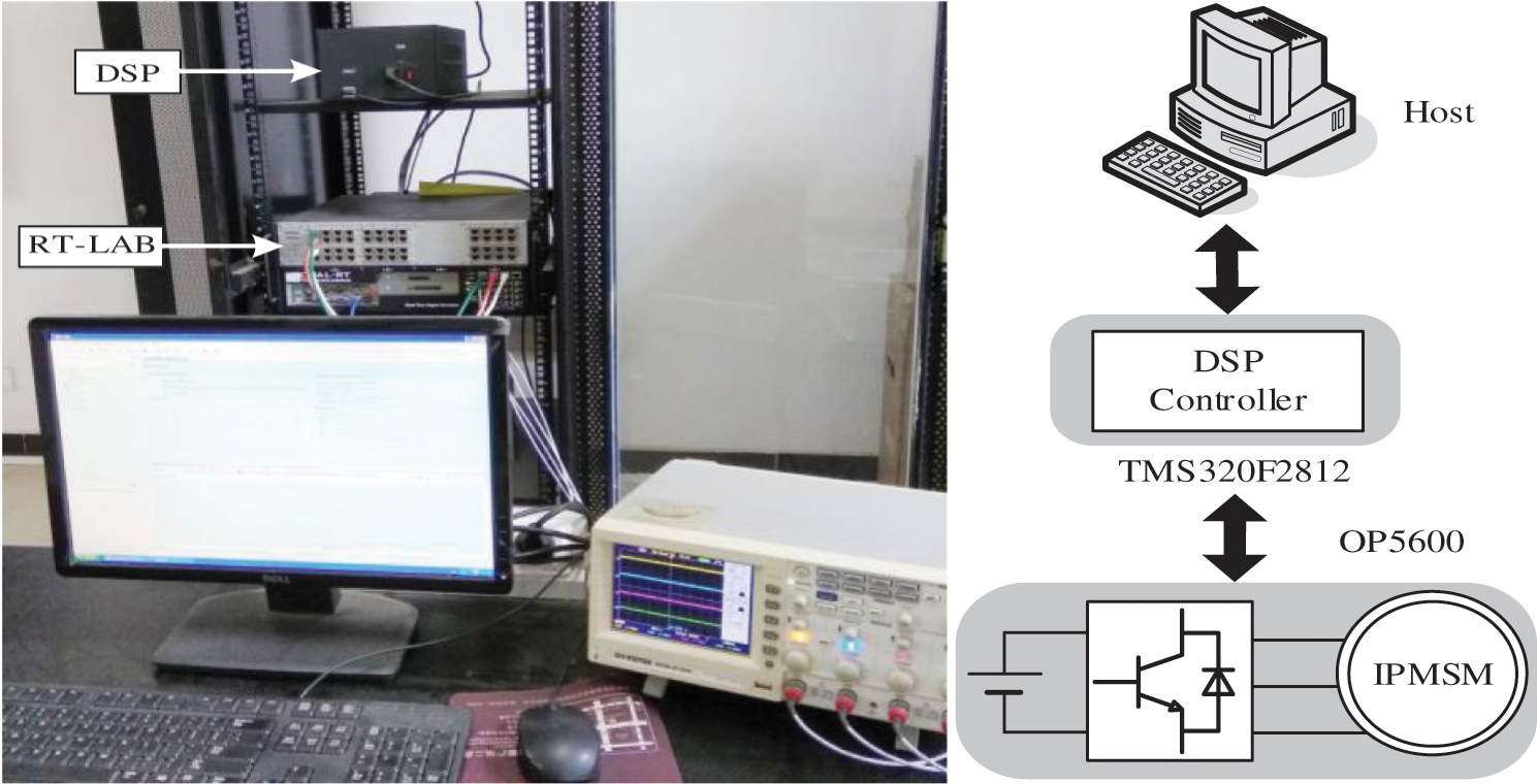
Figure 9: RT-Lab (OP5600) HILS experimental platform
Fig. 10 demonstrates the experimental results of PI, SMC and NFTSMC with graded speed regulation and uniform acceleration, respectively.
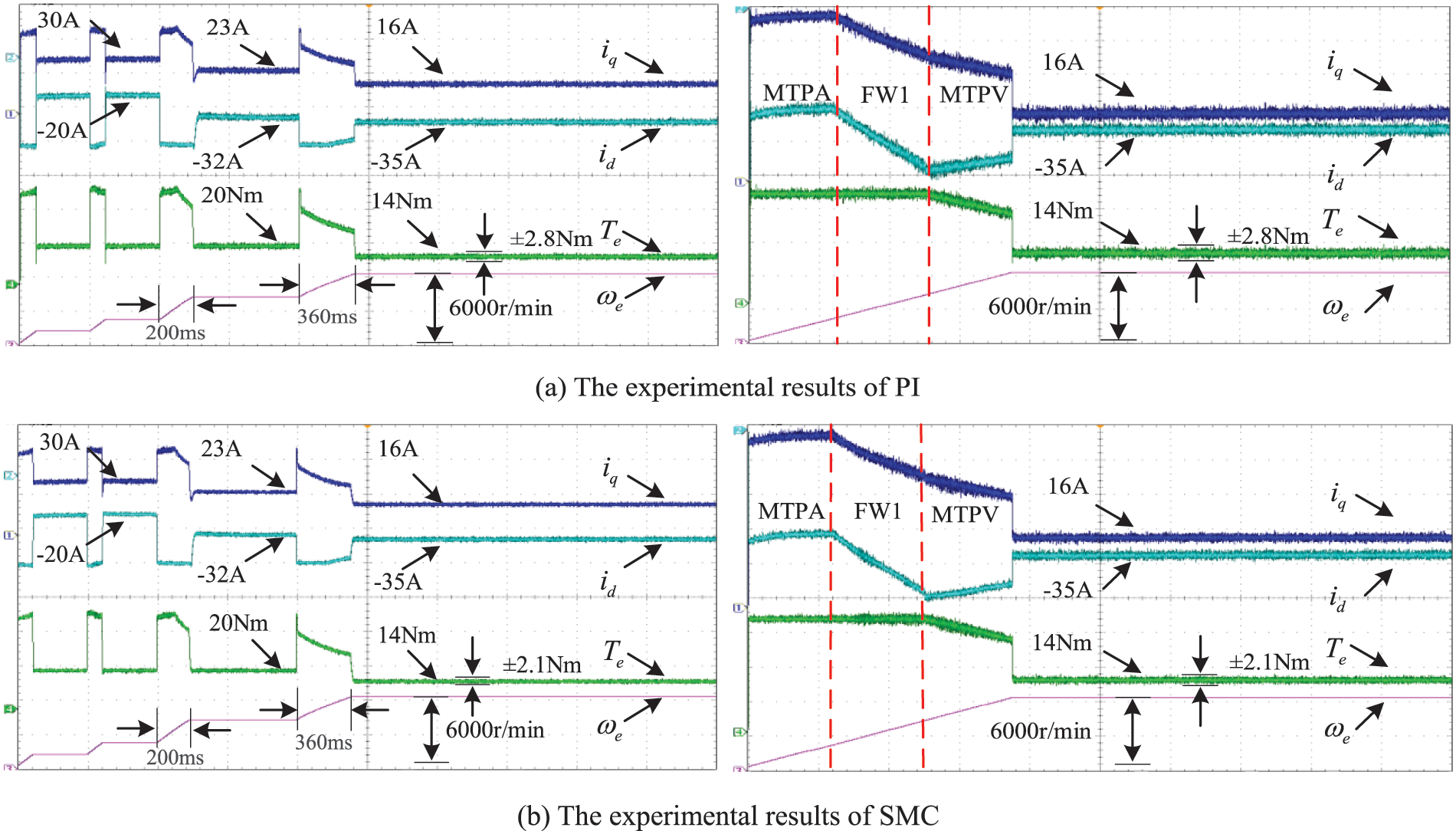
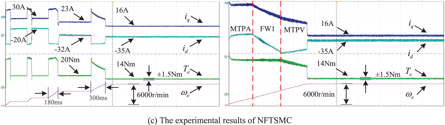
Figure 10: The experimental results of PI/SMC/NFTSMC with different working conditions
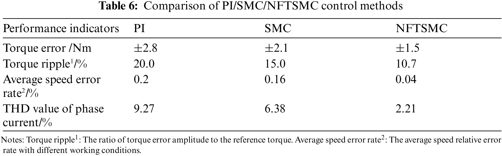
Compared with both Figs. 6 and 8, the control performance of the experiments is slightly decreased. Besides, the current pulsation and torque pulsation are more obvious in the transient condition, but the basic trend and effect comparison is consistent with the simulation results. As is shown in Fig. 10 and Table 6, the THD value of stator current for NFTSMC is the smallest. In addition, the average speed error rate of PI is 0.2%, and the average speed error rate of SMC is about 0.16%, while the average speed error rate of NFTSMC is only 0.04%. It indicates that NFTSMC has a better control accuracy. The torque ripple of PI is 20.0%, and the torque ripple of SMC is 15.0%, while the torque ripple of NFTSMC is only about 10.7% which is the smallest. The speed loop controller’s current pulsation of q-axis output is the leading cause of the torque ripple. Because NFTSMC can accurately track the reference speed, the actual current pulsation of the d-q axis and torque pulsation is effectively minimized.
This paper presents a novel NFTSMC based on deep flux weakening switching point tracking of FW control for IPMSM drive system. The deep flux weakening switching point is accurately obtained, and the NFTSMC speed controller is designed based on the input and the output to accelerate speed convergence. The unknown part of external disturbances is estimated quickly by ESMDO, which is fed back to the NFTSMC speed controller. The comparative analysis results of simulations and experiments indicate that the method proposed has excellent speed response. In addition, it can effectively minimize the current and torque pulsation, and the IPMSM drive system has better transient steady-state performance.
Funding Statement: This work was partly supported by the Natural Science Foundation of China under Grant No. 61733004 and the Scientific Research Fund of the Hunan Provincial Education Department under Grand No. 18A267.
Conflicts of Interest: The authors declare that they have no conflicts of interest to report regarding the present study.
References
1. Tang, R. Y. (2016). Modern permanent magnet machines: Theory and design. China: China Machine Press. [Google Scholar]
2. Wei, Y. H., Luo, X., Zhu, L., Zhao, J. (2021). Research on current harmonic suppression strategy of high saliency ratio permanent magnet synchronous motor based on proportional resonance controller. Proceedings of the CSEE, 7, 2526–2538. DOI 10.13334/j.0258-8013.pcsee.200697. [Google Scholar] [CrossRef]
3. Zhao, K. H., Zhang, C. F., He, J., Li, X. F., Feng, J. H. et al. (2017). Accurate torque-senseless control approach for interior permanent-magnet synchronous machine based on cascaded sliding mode observer. Journal of Engineering, 2017(7), 376–384. DOI 10.1049/joe.2017.0160. [Google Scholar] [CrossRef]
4. Chen, Y. Z., Huang, X. Y., Wang, J., Niu, F., Zhang, J. et al. (2018). Improved flux-weakening control of IPMSMs based on torque feedforward technique. IEEE Transactions on Power Electronics, 33(12), 10970–10978. DOI 10.1109/TPEL.2018.2810862. [Google Scholar] [CrossRef]
5. Pan, C. T., Sue, S. M. (2005). A linear maximum torque per ampere control for IPMSM drives over full-speed range. IEEE Transactions on Energy Conversion, 20(2), 359–366. DOI 10.1109/TEC.2004.841517. [Google Scholar] [CrossRef]
6. Carlos, M. E., Daniel, H. P., Gabriel, G., Marc, L. M., Daniel, M. M. (2020). Maximum Torque per Voltage Flux-Weakening strategy with speed limiter for PMSM drives. IEEE Transactions on Industrial Electronics, 68(10), 9254–9264. DOI 10.1109/TIE.2020.3020029. [Google Scholar] [CrossRef]
7. Li, K., Gu, X., Liu, X. D., Zhang, C. H. (2016). Optimized flux weakening control of IPMSM based on gradient descent method with single current regulator. Transactions of China Electrotechnical Society, 31(15), 8–15. DOI 10.19595/j.cnki.1000-6753.tces.2016.15.002. [Google Scholar] [CrossRef]
8. Lin, F. J., Liao, Y. H., Lin, J. R., Lin, W. T. (2021). Interior permanent magnet synchronous motor drive system with machine learning-based maximum torque per ampere and flux-weakening control. Energies, 10(2), 346. DOI 10.3390/en14020346. [Google Scholar] [CrossRef]
9. Zhang, Z. S., Wang, C. C., Zhou, M. L. (2020). Parameters compensation of permanent magnet synchronous motor in flux-weakening region for rail transit. IEEE Transactions on Power Electronics, 35(11), 12509–12521. DOI 10.1109/TPEL.2020.2987030. [Google Scholar] [CrossRef]
10. Xia, C. Y., Sadiq, U. R., Liu, Y. (2020). Inter-turn fault diagnosis of permanent magnet synchronous machine considering model predictive control. Proceedings of the CSEE, 40(S1), 303–312. DOI 10.13334/j.0258-8013.pcsee.191394. [Google Scholar] [CrossRef]
11. Zhao, K. H., Dai, W. K., Zhou, R. R., Leng, A. J., Liu, W. C. et al. (2022). Novel model-free sliding mode control of permanent magnet synchronous motor based on extended sliding mode disturbance observer. Proceedings of the CSEE, 42(6), 2375–2386. DOI 10.13334/j.0258-8013.pcsee.210273. [Google Scholar] [CrossRef]
12. Liu, J. H., Gong, C., Han, Z. X., Yu, H. Z. (2018). IPMSM model predictive control in flux-weakening operation using an improved algorithm. IEEE Transactions on Industrial Electronics, 65(12), 9378–9387. DOI 10.1109/TIE.2018.2818640. [Google Scholar] [CrossRef]
13. Glac, A., Šmídl, V., Peroutka, Z. (2018). Optimal feedforward torque control of synchronous machines with time-varying parameters. 44th Annual Conference of the IEEE Industrial Electronics Society, pp. 613–618. Washington DC, USA, IEEE. DOI10.1109/IECON.2018.8595139 [Google Scholar] [CrossRef]
14. Hammoud, I., Hentzelt, S., Oehlschlaegel, T., Kennel, R. (2020). Long-horizon direct model predictive control based on neural networks for electrical drives. The 46th Annual Conference of the IEEE Industrial Electronics Society, pp. 3057–3064. Singapore. DOI10.1109/IECON43393.2020.9254388 [Google Scholar] [CrossRef]
15. Liu, G. H., He, F. Y., Wu, X., Wang, Y. (2018). Flux weakening control of interior permanent magnet synchronous motor based on slide mode controller. Power Electronics, 52(3), 82–85. [Google Scholar]
16. Akhil, R. S., Mini, V. P., Mayadevi, N., Harikumar, R. (2020). Modified flux-weakening control for electric vehicle with PMSM drive. IFAC PapersOnLine, 53(1), 325–331. DOI 10.1016/j.ifacol.2020.06.055. [Google Scholar] [CrossRef]
17. Elena, T., Edorta, I., Antoni, A., Iñigo, K., Jonathan, J. et al. (2017). PM-assisted synchronous reluctance machine flux weakening control for EV and HEV applications. IEEE Transactions on Industrial Electronics, 65(4), 2986–2995. DOI 10.1109/TIE.2017.2748047. [Google Scholar] [CrossRef]
18. Zhao, Y., Liu, B. (2017). Flux-weakening vector control of interior permanent magnet synchronous motor based on sliding mode variable structure controller. Information and Control, 46(4), 428–436 442. DOI 10.13976/j.cnki.xk.2017.0428. [Google Scholar] [CrossRef]
19. Liu, B., Zhao, Y., Hu, H. Z. (2018). Structure-variable sliding mode control of interior permanent magnet synchronous motor in electric vehicles with improved flux-weakening method. Advances in Mechanical Engineering, 10(1), 168781401770435. DOI 10.1177/1687814017704355. [Google Scholar] [CrossRef]
20. Zhao, K. H., Yin, T. H., Zhang, C. F., He, J., Li, X. F. et al. (2019). Robust model free nonsingular terminal sliding mode control of PMSM demagnetization fault. IEEE Access, 7, 15737–15748. DOI 10.1109/ACCESS.2019.2895512. [Google Scholar] [CrossRef]
21. Li, K., Wang, Y. (2019). Maximum torque per ampere (MTPA) control for IPMSM drives using signal injection and an MTPA control law. IEEE Transactions on Industrial Informatics, 15(10), 5588–5598. DOI 10.1109/TII.2019.2905929. [Google Scholar] [CrossRef]
22. Shi, M., Feng, J. H., Xu, J. F., He, Y. P., Xiao, L. (2015). Research of permanent magnet synchronous motor control stability improving in depth flux-weakening area. Electric Drive for Locomotives, 1, 22–25. DOI 10.13890/j.issn.1000-128x.2015.01.006. [Google Scholar] [CrossRef]
23. Sheng, Y. F., Yu, S. Y., Gui, W. H., Gong, Z. N. (2010). Field weakening operation control strategies of permanent magnet synchronous motor for railway vehicle. Proceedings of the CSEE, 30(9), 74–79. DOI 10.13334/j.0258-8013.pcsee.2010.09.009. [Google Scholar] [CrossRef]
24. Zhu, L. D., Wang, X., Zhu, H. Q. (2020). An IPMSM deep flux weakening algorithm with calculable parameters to avoid out-of-control. Proceedings of the CSEE, 40(10), 3328–3336. DOI 10.13334/j.0258-8013.pcsee.190945. [Google Scholar] [CrossRef]
25. Wang, Y. Q., Zhu, Y. C., Feng, Y. T., Tian, B. (2021). New reaching law sliding-mode control strategy for permanent magnet synchronous motor. Electric Power Automation Equipment, 41(1), 192–198. DOI 10.16081/j.epae.202010005. [Google Scholar] [CrossRef]
26. Xu, B., Zhang, L., Ji, W. (2021). Improved non-singular fast terminal sliding mode control with disturbance observer for PMSM drives. IEEE Transactions on Transportation Electrification, 7(4), 2753–2762. DOI 10.1109/TTE.2021.3083925. [Google Scholar] [CrossRef]
27. Zhao, K. H., Liu, W. C., Yin, T. H., Zhou, R. R., Dai, W. K. et al. (2021). Model-free sliding mode control for PMSM drive system based on ultra-local model. Energy Engineering, 119(2), 767–780. DOI 10.32604/EE.2021.018617. [Google Scholar] [CrossRef]
Cite This Article
 Copyright © 2023 The Author(s). Published by Tech Science Press.
This work is licensed under a Creative Commons Attribution 4.0 International License , which permits unrestricted use, distribution, and reproduction in any medium, provided the original work is properly cited.
 Downloads
 Citation Tools