A Novel Ultra Short-Term Load Forecasting Method for Regional Electric Vehicle Charging Load Using Charging Pile Usage Degree

1  Introduction

Environment-friendly EVs are being developed vigorously to deal with environmental challenges as the fast growth of global economy [1]. With the development of battery EVs, the energy consumption demand for transportation will gradually shift to the power grid, which will inevitably impose a great burden on the original power grid [2]. It is especially important to guide the charging behavior of EVs in order to prevent a sudden and extremely large power spike in the grid and to relieve the pressure on the grid. Guiding EV charging and power dispatching cannot be done without load forecasting [3,4]. Therefore, the current EV charging load research areas include charging load forecasting [5], charging load scheduling, etc. Hence the impact of these residential loads on power distribution systems should be analyzed and dealt with proper measures. Accurate load forecasting results are the most important precondition for these measures [3,4].

Traditional electric load forecasting methods are mainly used to predict the system-level loads based on the periodic characteristics and stochastic of the predicted load [5]. These load forecasting methods can be mainly divided into model-driven and data-driven methods. In the model-driven methods, a number of independent variables are selected to produce a dependent variable, which is the predicted electric load, such as the multiple linear regression-based forecasting method [6]. In the data-driven methods, the historical load data is dealt with several algorithms, including traditional time series algorithm [7], data smoothing algorithms [8], and artificial intelligence algorithms [9–15]. The key factors related to the electric load should be identified properly in model-driven load forecasting methods. In the field, these factors are always hard to collect by the engineers. Data-driven methods can be easily realized once enough historical load data is sampled and stored, but the forecasting error may increase obviously if one or more influencing factors vary unexpectedly.

The focus of the charging load forecasting area is mainly on improving the accuracy of load forecasting. EV charging loads have similar characteristics to traditional loads, so the load forecasting methods applied to traditional loads are also widely used for EV charging loads. The charging load forecasting methods for EVs are also mainly divided into data-driven and model-driven methods, but load characteristics and influencing factors of EV charging loads have many specialties. The traditional electricity load generally shows a peak during the day and a low at night. As for the EV charging load, the EV charging load is less regular due to the spatial and temporal randomness of EV charging [16]. Reference [17] proposed a clustering multi-node learning method based on Gaussian process for fusing data from multiple charging stations to improve load prediction accuracy. Reference [18] proposed a data-driven load forecasting method for large-scale EV charging load forecasting. These studies above are improvements on data-driven methods, and it is difficult to further improve the forecasting accuracy because they do not take full advantage of the load mechanism of EVs, combined with the advantages of model-driven methods. EV charging load is significantly influenced by traffic situations, weather conditions [19], etc. And due to the diversity of transportation modes, the frequency of use and charging load size of EVs are more elastic to change. In the meantime, EV power batteries are more closely correlated with environmental factors such as temperature [20]. The above shows that most of the electric vehicle charging load forecasting focuses on regional charging load forecasting, and a few literature focus on charging station load forecasting [21].

Due to the lack of real data for EV charging load, regional EV load forecasting methods mainly focus on model-driven methods. Specifically, combined with the charging characteristics of EVs, the spatial and temporal distribution characteristics of EVs are simulated to establish a corresponding load forecasting model [22,23]. There is literature to forecasting the load by studying the battery condition of EVs [24]. With the collection of charging pile data, the existing artificial intelligence algorithm is applied to the charging load forecasting of EV [25]. Compared with traditional model-driven methods, the data-driven methods have the advantages of comprehensive utilization of historical data, simplification of EV charging load forecasting model, and no need to assume a large number of model parameters [26].

Among the data-driven short-term load forecasting (STLF) methods, there are usually two stages, which include the data preprocessing stage and the load forecasting stage. In reference [2], within-day and within-week seasonalities are specially extracted from the raw data and several forecasting algorithms are performed on the filtered series, including autoregressive models, double seasonal Holt-Winters exponential smoothing algorithms, Echo state network-based model, wavelets algorithms, and multiple linear regression models. In reference [27], the support vector machine is selected to achieve the STLF results. The climatic factors are specially preprocessed as the input parameter of the forecasting model, and the grasshopper optimization algorithm is introduced to evaluate the suitable parameters. Since the single residential load has strong randomness and high volatility, characteristics of residential load are analyzed by [28–30], and several deep learning models are applied to achieve STLF results of residential loads. The results show that the prediction error of residential loads is bigger than that of system-level loads. Specific preprocessing measures and novel deep learning models can improve the prediction accuracy by the validation of many scholars.

In fact, each charging pile in the region has its own unique power consumption characteristics during the day. During the day, the peak and trough charging periods of charging pile are different, and the frequency of use is also very different. The average load of the charging pile at the same time point on different days reflects the frequency of use of the charging pile at this time point, and on the contrary, the higher the frequency of use of the charging pile, the probability that the charging pile will be used at the same time point in the future will also increase, so there is a large probability of charging the charging pile at the same time point in the future. The average load at the same point in time on different days of the charging pile load forecasting. To improve the accuracy of the ultra short-term regional EV charging load forecasting results, a hybrid model and data-driven forecasting method is proposed and realized in this paper. The charging pile usage degree is defined and obtained by analyzing the daily usage curve of each charging pile. The charging pile usage degree would be used as the indicator for the traffic condition. Firstly, the abnormal EV charging daily load is removed by the Density-Based Spatial Clustering of Application with Noise (DBSCAN) clustering algorithm. Secondly, the load value of the charging pile is encoded to obtain the charging pile usage degree at each moment. Thirdly, the long-short term memory (LSTM) load forecasting model is constructed to deal with the charging pile usage degree and the historical charging load data. Fourthly, a novel ultra short-term forecasting method of EV charging loads is realized and verified by the field data. Finally, the load forecasting accuracy is directly influenced by the load fluctuation, this paper presents a load characteristic index for the fluctuation of adjacent day load and adjacent week load, which can be used to determine the mean absolute percentage error (MAPE) size of the forecasting result before forecasting and description of load fluctuation characteristics.

In Section 2, the method of load forecasting using charging pile usage degree is given. The definition of charging piles and the calculation steps are explained in detail. The average load of charging piles at the same point in time on different days is useful for load forecasting, and the average load of charging piles at the same point in time on different days is further coded in this paper to obtain the charging pile utilization.

In Section 3, the simulation analysis is carried out. The load characteristics of EV charging loads in small areas are analyzed, and the various results of the charging post usage calculation process are shown. The load forecasting methods in this paper are compared with the traditional load forecasting methods from the perspective of EV charging loads in different months and different scales.

In Section 4, the conclusion is drawn. The full paper is summarized, concluding that the load forecasting method in this paper is effective, and looking ahead.

2  Regional Charging Pile Utilization and EV Charging Forecasting Method

The charging conditions of EVs applied by our method is shown in Fig. 1. Each charging station uploads its own signals to the dispatching center, including the charging load data of EVs. The dispatching center predicts the regional charging load of EV according to the uploaded signals of all charging stations in the predicted area. According to the accurate prediction results, the scheduling plan of regional charging load can be derived to realize the optimal vehicle to grid benefit, such as the optimal demand response of EV charging load.

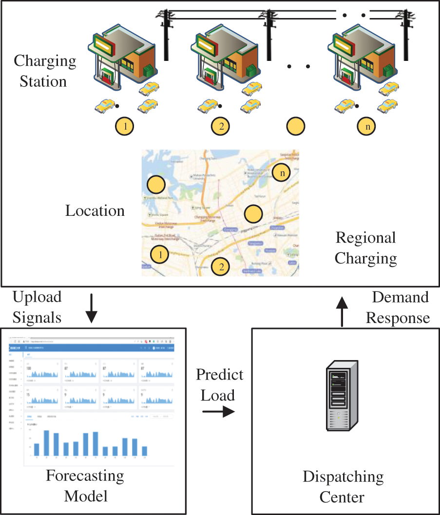
Figure 1: Regional EV charging load prediction and its application

2.1 Definition of Charging Pile Usage Degree

In fact, each charging pile in the region has its own unique power consumption characteristics during the day. During the day, the peak and trough charging periods of charging pile are different, and the frequency of use is also very different. The average load of the charging pile at the same time point on different days reflects the frequency of use of the charging pile at this time point, and on the contrary, the higher the frequency of use of the charging pile, the probability that the charging pile will be used at the same time point in the future will also increase, so there is a large probability of charging the charging pile at the same time point in the future. The average load at the same point in time on different days of the charging pile load forecasting. However, due to the complexity of the load, directly inputting the average load at the same point in time on different days into the data-driven load forecasting model will increase the complexity of the network, which is prone to overfitting, and instead does not yield better forecasting results. In this paper, the average load of charging piles at the same time point on different days is further coded to reduce the complexity of the data. This paper integrates the charging load mechanism of charging piles in a data-driven approach, and proposes a load forecasting method based on the usage degree of charging piles, which integrates the advantages of data-driven and model-driven and improves the forecasting accuracy.

The key influencing factor of EV charging load is the EV traffic information. The concept of the average daily usage degree of charging piles, CSw is proposed by us for the first time. And the degree of traffic information influence in this paper is mainly derived by analyzing the average daily usage degree of each charging pile.

The average load of the EV charging pile in each small period can be used to reflect the usage degree of the charging pile at each moment. It is determined by the arrival times of EVs at charging stations at each moment, which indirectly reflects the nearby traffic condition. Therefore, the important information of charging pile usage degree is extracted as a key input variable for charging load prediction.

The steps of regional charging pile usage degree extraction work are given as follows:

(1)   There is certain regularity in the daily EV charging load at the regional level. The abnormal daily load is removed by the DBSCAN clustering algorithm. If cluster analysis results show that o day’s loads are outliers in the whole N day’s regional charging loads, the number of days with regular EV charging load is N-o days. And the load in the ith day belonging to the regular days is denoted as Pc,i.

DBSCAN is a density-based clustering technique, and its advantage is that it does not require a preset number of clusters and can be used to identify outliers from a set of daily load curves [31]. Hence it is suitable to eliminate abnormal EV charging daily loads.

(2)   Calculate the average load values Pht¯ and Pwt¯ of charging piles at each time on holidays and workdays in the regular days, respectively. The average load values Pht¯ and Pwt¯ at each time during holidays and workdays are used to form the series of average daily loads Ph¯ and Pw¯.

Pwt¯=1w∑i=1wPit(1)

Pw¯=[Pw1¯,Pw2¯,Pw3¯,⋅⋅⋅,Pwt¯,⋅⋅⋅,Pwe¯](2)

Pht¯=1h∑i=1hPit(3)

Ph¯=[Ph1¯,Ph2¯,Ph3¯,⋅⋅⋅,Pht¯,⋅⋅⋅,Phe¯](4)

(3)   There are s charging piles in the whole region. The average daily load of the first charging pile during holidays and workdays is recorded as Ph¯1 and Pw¯1, respectively. Then the average daily load of the sth charging pile during holidays and workdays is Ph¯s and Pw¯s, respectively. The average daily load distribution Sw of all charging piles in the region in workdays is given as follows:

Sw=[Pw¯1Pw¯2⋮Pw¯s]=[Pw1¯1Pw2¯1⋯Pwe¯1Pw1¯2Pw2¯2⋯Pwe¯2⋮⋮⋱⋮Pw1¯sPw2¯s⋯Pwe¯s](5)

where Pwi¯j represents the average load at time i of the j-th charging pile on a working day.

(4)   The load of each charging pile varies in a wide range, and it cannot be directly used as the input parameter of the deep learning-based forecasting model. These load data would be encoded as a new time series. The maximum element in the obtained matrix Sw can be found and equals Psw.max, and the minimum element in the obtained matrix Sw equals Psw.min. Then any load data Pload would be encoded as Cpload, and the calculation algorithm is given as

mPload=round(Pload−Psw.minPsw.max−Psw.min×NI)(6)

Cpload=[Psw.min+(mPload+0.5)×Psw.max−Psw.minNI]×k+b(7)

where NI represents the total divided number of the sections from the minimum value Psw.min to the maximum value Psw.max; function round (x) represents a function that rounds each element of x to the nearest integer at the left of the decimal point; mPload represents the located number of the sections related to the load Pload; Cpload represents the encoded value related to the load Pload, which is located from 1 to 100; variables k and b represent the coefficients in the encoded process.

Therefore, the average daily load distribution Sw of all charging piles in the region in workdays would be encoded and transformed into

CSw=[CPw¯1CPw¯2⋮CPw¯S]=[CPw1¯1CPw2¯1⋯CPwe¯1CPw1¯2CPw2¯2⋯CPwe¯2⋮⋮⋱⋮CPw1¯sCPw2¯s⋯CPwe¯s](8)

(5)   The encoded value curve of average usage degree of the charging piles in the whole region in workdays can be obtained by the encoded values of each charging pile, which is calculated by

Cpile=[Cpile,1Cpile,2⋯Cpile,e](9)

Cpile,m=∑i=1sCPwm¯i(10)

(6)   The encoded value curve of average usage degree of the charging piles in the whole region in holidays can be obtained by repeating the steps from 1 to 5. And then the encoded value curve of average usage degree of the charging piles in the whole region for the historical data can be obtained as a complete time series X of the regional charging pile usage degree indicator.

2.2 LSTM-Based EV Charging Load Forecasting Model

LSTM is a kind of recurrent neural network (RNN) and is realized based on the general recurrent neural network. The internal structure of LSTM is improved so that it can maintain the long-range dependence of time series and effectively avoid gradient disappearance and gradient explosion. In this paper, LSTM is selected to construct the EV charging load forecasting model.

The historical EV charging load data L and charging pile usage degree X are selected as the input variables for the load prediction model. The structure of the prediction model built in this paper is shown in Fig. 2a.

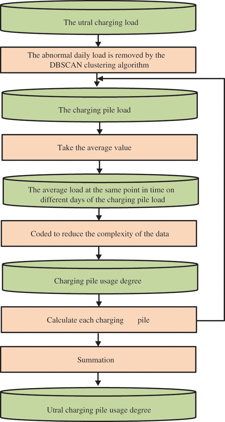
Figure 2: Charging pile usage degree calculation process

The EV charging load data and charging pile usage degrees need to be normalized to simplify the computation during training and speed up the network convergence before feeding the dataset into the model. The normalization formula is given as follows:

Pintnorm=Pint−PminPmax−Pmin(11)

Cpile,mnorm=Cpile,m−Cpile,minCpile,max−Cpile,min(12)

where Pintnorm and Cpile,mnorm represent the normalized value of the EV charging load and encoded value of the usage degree of regional charging piles, respectively; Pint and Cpile,m represent the initial values of the EV charging load and usage degree of regional charging piles, respectively; Pmin and Pmax represent the minimum and maximum of the input series of the EV charging load, respectively; Cpile,min and Cpile,max represent the minimum and maximum of the input series of the usage degree of regional charging piles.

The input variables are fed into the LSTM for training after normalization. The constructed load prediction LSTM network consists of 1 input layer, 2 hidden layers, and 1 output layer. The input layer contains 2 cells and each hidden layer contains 20 memory cells.

The LSTM learning rate is used to control the learning progress of the model. A small learning rate will increase the learning time of the network, and a large learning rate may make the network to have difficulties in finding the optimal value and the network cannot converge. In this paper, the learning rate is selected empirically.

2.3 EV Charging Load Forecasting Results Assessment

In the field, the load forecasting accuracy at the system level is obviously higher than that of power distribution networks. Indeed, the load forecasting accuracy is directly influenced by the load fluctuation, and strong periodicity would improve the prediction accuracy. For different type loads, the fluctuant components proportion is different. In our paper, regional EV charging load has high randomness and strong volatility. In the same area, the forecasting error of EV charging load is generally bigger than that of regular distribution electric load. Therefore, when traditional load forecasting methods are used to predict EV charging load, the MAPE would change. In this paper, in addition to MAPE being used to assess load forecasting errors, some metrics to characterize the adjacent day and adjacent week volatility of the historical data of the load to be forecast are proposed. It is convenient to confirm whether the load data can achieve satisfactory results when they are input into the forecasting model before the forecasting.

Load characteristic indexes include load fluctuation rate, load rate, peak-to-valley difference, etc. These load characteristic indexes describe the characteristics of the intra-day load or the load characteristics of the total historical data amount in the load history N days to be analyzed. In the charging load characteristic index, there is no clear index of the difference between adjacent day load and adjacent week load, there is also no clear index to confirm whether the load data input forecasting model can achieve better results before forecasting. In the load forecasting model, the input data even if the day load volatility is large, but the adjacent day load volatility or adjacent week load volatility is small, can also explain the load has certain regularity, and the forecasting effect is not necessarily poor. It is important to use indexes to describe adjacent day load fluctuation and adjacent week load fluctuation. The traditional load fluctuation rate is Eq. (13).

FLi=1Pavg∑s0=1S(Ps0−Pavg)2S−1(13)

where FLi denotes load fluctuation rate, Pavg represents the average of the total historical data amount in the N-day of the load to be analyzed, Pavg=1S∑s0=1SPs0. S represents the total historical data amount in N days of the load to be analyzed and then equal to N × T, T represents the interval time ΔT of 24 h in load monitoring, general ΔT equal to 30 min, at this time, T equal to 48. N represents the total number of days in the historical load data to be analyzed, Ps0 represents the load value of the s0-th data in the load data to be analyzed.

This paper presents a load characteristic index for the fluctuation of adjacent day load and adjacent week load, considering the difference between adjacent day load and adjacent week load. Accumulate the ratio of the load difference between different adjacent days and adjacent weeks at the same time to the total daily load and total weekly load, respectively. Therefore, it is convenient to confirm whether the load data can achieve satisfactory results when they are input into the forecasting model before the forecasting. The adjacent day load fluctuation rate and the adjacent week load fluctuation rate are defined as Eqs. (14) and (15), respectively.

FLd=∑i=1N−1∑t0=1T|Pi+1(t0)−Pi(t0)|∑t0=1TPi(t0)(14)

FLw=∑i=1N−1∑t0=1T|Pi+7(t0)−Pi(t0)|∑t0=1TPi(t0)(15)

where FLd denotes adjacent day load fluctuation rate, FLw denotes adjacent week load fluctuation rate. Pi(t0) represents the load power to be analyzed at time t0 on day i, t0 × ΔT = t, s0 = i × T + t0.

In summary, FLi describes the difference between each load value and the average load value, reflects the overall fluctuation of N-day historical load data, but cannot reflect the load data adjacent day and adjacent week have regularity. FLd describes the difference between all adjacent days at the same moment, FLw describes the difference between all adjacent weeks at the same moment, it can show the magnitude and regularity of the fluctuation of adjacent days and adjacent weeks of load data.

MAPE as the cost function in this paper, the training process of the load forecasting model reduces the MAPE of the forecasting results. The specific formulas for RMSE and MAE are listed below:

MAPE=100%n∑i=1n|y^i−yiyi|(16)

RMSE=1n∑i=1n(y^i−yi)2(17)

MAE=1n∑i=1n|y^i−yi|(18)

where yi^ is the predicted value and yi is the true value. n represents the number of prediction results.

2.4 LSTM-Based EV Charging Load Forecasting Framework

The overall forecasting process is shown in Fig. 3b. Firstly, the original transaction data of EV charging stations is prepossessed to obtain the EV charging load series. Secondly, the usage degree of the charging piles is analyzed and obtained by the proposed method mentioned in Section 2.1. Thirdly, the input variables of the proposed LSTM-based EV charging load forecasting model are obtained by the combination of the EV charging load data and the usage degree data of charging piles. Fourthly, the LSTM load forecasting model is constructed to deal with the whole EV forecasting task. Finally, assessment of load forecasting results, comparison of MAPE, and load characteristic indexes.

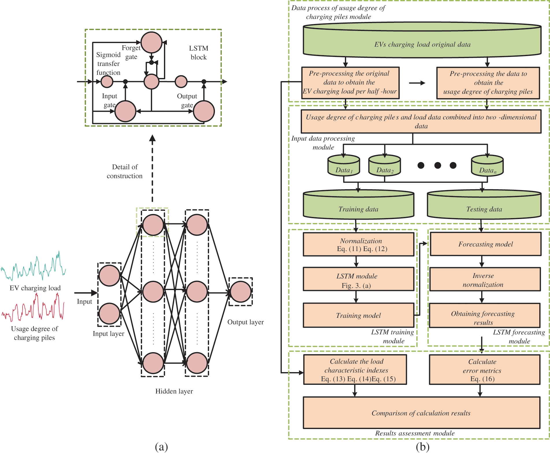
Figure 3: Charging load forecasting model and process of EV (a) the structure of the LSTM-based EV charging forecasting model; (b) our proposed ultra short-term EV charging load forecasting flow chart

3  Case Study

3.1 EV Charging Load Datasets and Data Preprocessing Work

The transaction data of all EV charging stations in some region in the field is collected by us in Hubei province. The EV charging stations can be divided into two categories based on their operating locations, including urban charging stations and highways circumjacent charging stations. In addition, the EV charging transaction data includes the start time of the charging process, power consumption of the charging process, the charging cost, the charging pile location, and the end time of the charging process.

Since the raw data is recorded in transaction order format, it is necessary to perform the data preprocessing work to obtain the charging load in time series firstly.

Specific preprocessing efforts for the EV charging transaction data include the following steps:

(1)   Reorder each transaction order into a column by the start and end time, and divide the transaction power consumption by the total charging time to express the average charging power for that period.

(2)   The start and end times of these charging transaction orders are relatively random and the charging time is inconsistent, which is not conducive to conducting cluster and prediction studies. Hence interpolation process should be done to form the charging load in time series. Due to many charging times lasting only about two minutes, the expanded time scale is 1 min. Power data is interpolated with zero power supplement between two order times, and the charging power in one order is regarded as the same value.

We selected two-day daily load curves of urban charging stations and highways circumjacent charging stations in a region, and it is shown in Fig. 4. It can be found that the charging load of urban charging stations exists almost all day long, with the peak value appearing after eight o'clock in the evening and the trough value appearing after eight o'clock in the morning, the characteristics of the peak and trough value, which are inseparable from the travel behavior of residents. The highways circumjacent charging stations have almost no charging load throughout the day, and there is a charging load around 4 pm. The charging load of urban charging stations is significantly higher than that of highway circumjacent charging stations due to the higher number of urban EVs and the lower number of highway circumjacent EVs.

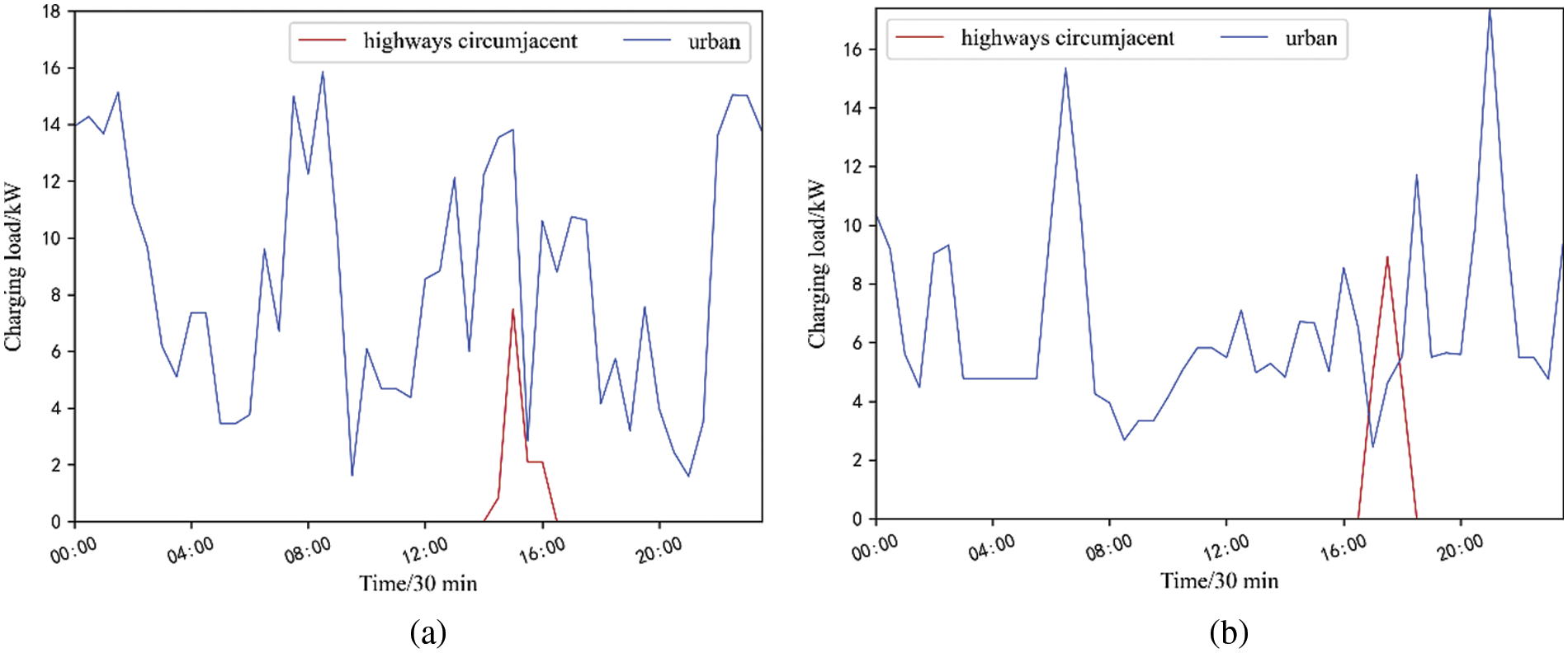
Figure 4: The typical daily charging load in urban charging stations and highways circumjacent charging stations (a) 01 October; (b) 30 December

3.2 Characteristics of Regional EV Charging Load

The regional EV charging load can be obtained after the preprocessing steps, and it is shown in Fig. 5. The specific regional charging load from January 16 to January 27 is shown in the figure, where the maximum charging load is 191.4 kW, the minimum is 10.9 kW, and the average is 82.9 kW. It can be found that in the half a month of January, the twenty-four hours’ overall variation law of EV charging load in a certain region between different days is strong, which has great similarity. There is a great similarity in the daily load curves for any two days for different days in a region. The peak and trough moments of load occur very close to each other in adjacent days, and the time periods of load rise and fall are also close to each other. Therefore, the similarity of the load curves on adjacent days is strong.

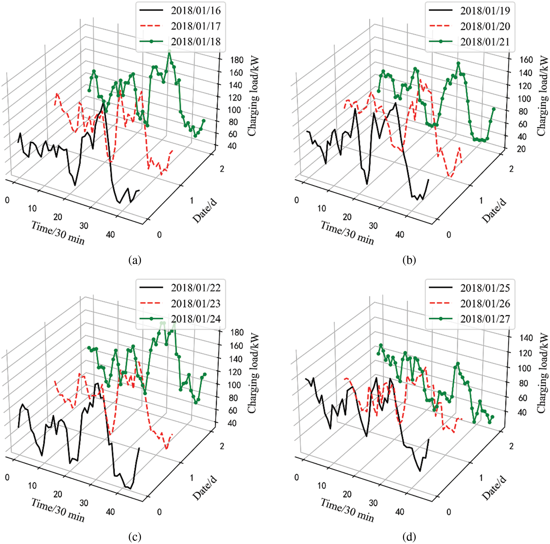
Figure 5: One regional EV charging load curve in the filed in (a) 16–18 January; (b) 19–21 January; (c) 22–24 January; (d) 25–27 January

There is a certain difference in the regional EV load between the workday and the holiday. Overall, the overall change of 24 h between different days has a strong regularity, which also shows that the load elements corresponding to the time points of the day are encoded as an input variable into the data-driven load forecasting model is reasonable. It also shows that it is necessary to take the day as the unit to extract the daily distribution of the use degree of EV charging piles in the region.

The EV load data can be divided into different regions according to the geographical location information. In this paper, the data of a small and a large region are used for analysis and research. The small filed contains 10 charging stations, and the large region contains 69 charging stations. Among them, the data of January in a small region are used as the basic data of simulation, and other data are used for comparative analysis and research.

The EV load box plot of holiday and workday in small region and large region is shown in Fig. 6. The uppermost circle in the figure represents the value of abnormal load, and the horizontal lines from top to bottom represent maximum value, third quartile, median, first quartile, and minimum value, respectively. It can be clearly found that the loads on holiday and workday are significantly different. The average load on workday is significantly greater than that on holiday. The maximum and minimum loads on workday in most months are higher than that on holiday. Therefore, it is necessary to distinguish between workday and holiday when extracting the information about EV charging piles usage degree, The distribution and change rules of the charging piles usage degree in the region on holiday and workday are respectively extracted.

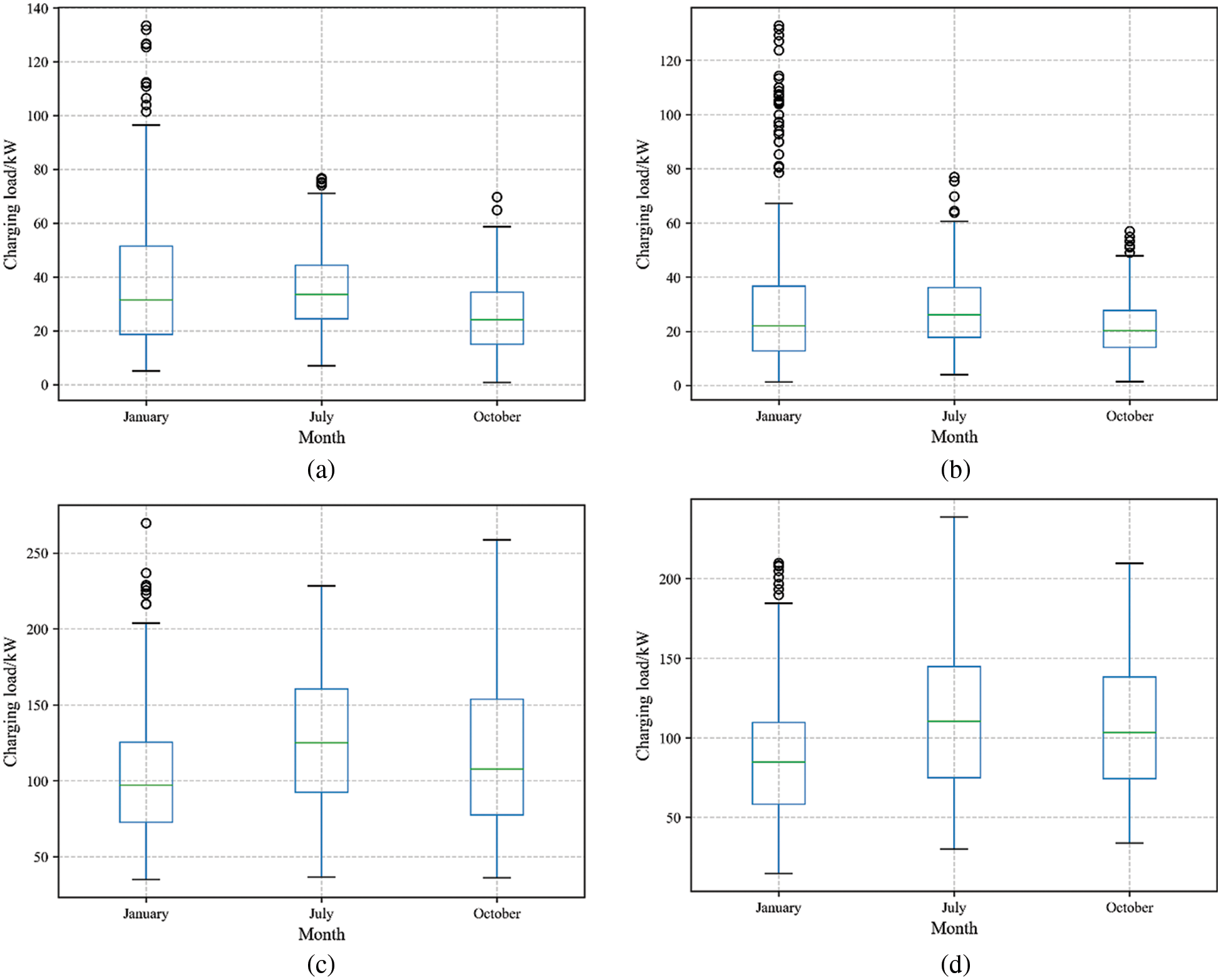
Figure 6: Box plot of EV charging load (a) Workdays in a small region; (b) Holidays in a small region; (c) Workdays in a large region; (d) Holidays in a large region

3.3 The Usage Degree of Regional Charging Pile

The DBSCAN clustering algorithm is used to analyze the total charging load of EVs in January. The clustering results are as shown in Fig. 7. It can be found that the daily EV charging load in a certain area is clustered into one cluster in January, and only the load on January 5 and 6 does not belong to the cluster. This shows that the pattern of EV charging load in a certain region is obvious among different days. However, the daily load curve of the same cluster also has certain differences, especially the charging loads in workdays and holidays when extracting the information of the use degree of EV charging piles. It can be found that the outlier load from zero to 3:00 pm is about twice of the other daily loads in Fig. 6b. Therefore, it is necessary to eliminate the outlier load when obtaining the charging pile usage degree, otherwise the calculated charging post usage can hardly reflect the regional EV usage pattern, and the calculated charging pile usage degree can hardly play its role when input to the load forecasting model, and the accuracy of load forecasting is not high.

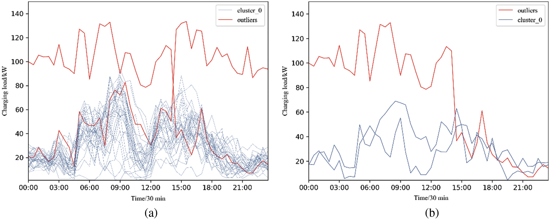
Figure 7: Clustering results of one regional EV charging load in January 2018 (a) 31 days; (b) 3 days

The load data of January 05 and 06 are removed from the load data of 88 EV charging piles in a certain area. And then the daily average load value is calculated in these regular days. The number of charging piles within the same range of charging load power is counted to identify the proper encoded value of the charging pile usage degree. The charging load power is firstly divided into several ranges with the interval of 0.05 kW, and then the boundary values of these ranges are adjusted by the statistical charging load power. The final divided ranges and the corresponding encoded values for the charging piles are given in Table 1. Where number represents the number of load values in the load-interval. There are 2873 load values in the load-interval of 0–0.049, and 0 is the largest number of load value, which exists in the load-interval of 0–0.049.

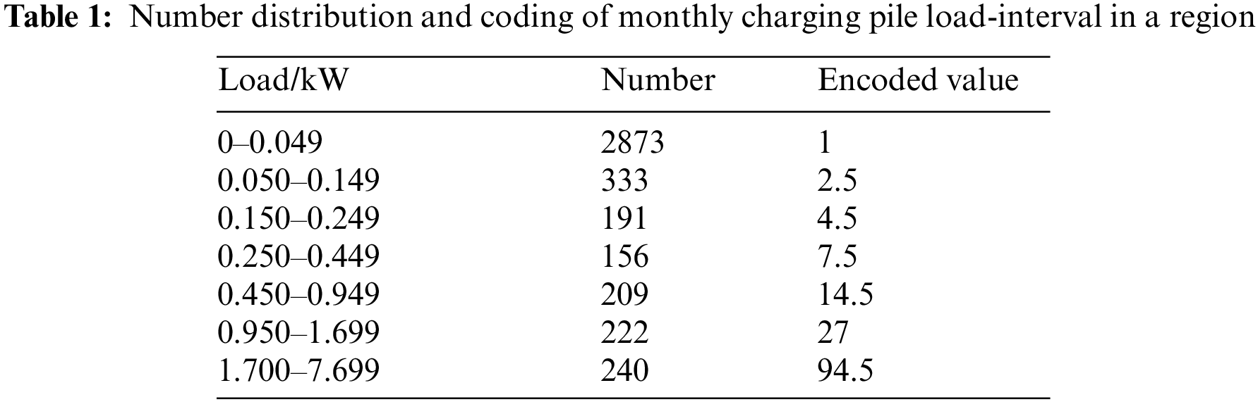
The specific method to obtain the usage degree of regional charging piles is in Section 2.1, k and b in Eq. (7) are taken as 20 and 0.5 respectively in the data we use.

The load value of different intervals is encoded by the multiple of the median value of the interval, which indicates the daily use of different charging piles.

The abnormal load in the daily load clustering results is removed from the daily load in January. Considering the different charging modes of holidays and working days, the daily average values of the charging pile load are calculated and plotted for holidays and weekdays. The sum of the encoded values of all charging piles in the selected region is obtained and used in the regional charging load forecasting. The results are shown in Fig. 8. The maximum the usage degree of regional charging pile in holidays is 994.5, and the maximum the usage degree of regional charging pile in workdays is 1632.5.

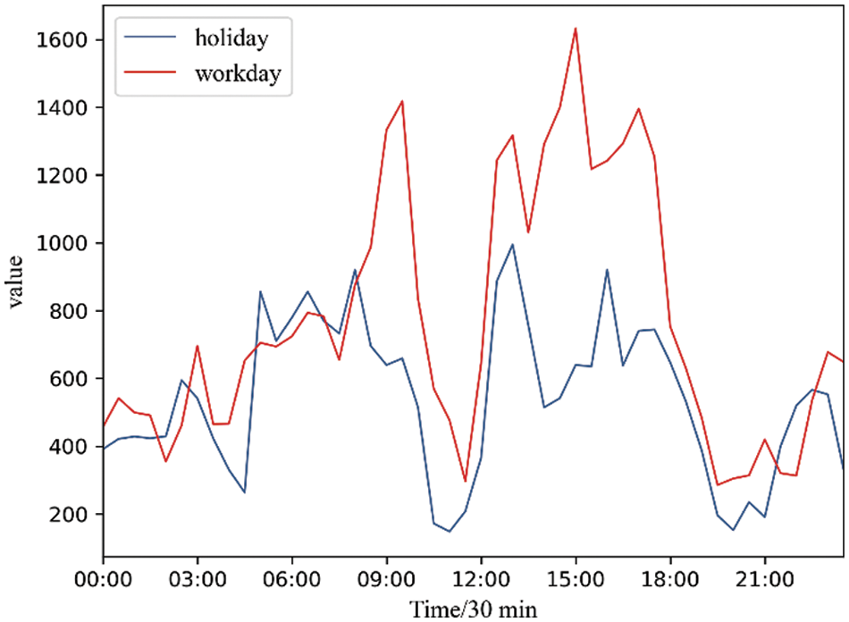
Figure 8: The encoded values of the usage degree of regional charging piles in January

It can be seen that the usage degree of regional daily charging piles in January is expressed as that the charging peak time is around 5 pm, and the usage degree of charging piles on workdays is significantly higher than that on holidays.

The regional average daily charging pile usage degree obtained above is replaced repeatedly according to the distribution of holidays and workdays to obtain a complete regional charging pile usage degree time series, which is consistent with the length of the regional charging load sequence in January. Then correlation analysis and load forecasting are studied.

The correlation between regional charging pile usage degree and regional EV charging load in January was 0.539. The Pearson correlation coefficient between 0.5 and 0.8 indicates a moderate correlation. There is a certain correlation between the extracted charging pile usage degree in January and the charging load of EVs. Therefore, it is feasible to input the charging pile usage degree as an input variable into the load forecasting model.

3.4 EV Charging Load Forecasting Results

The historical load data in January were selected for simulation analysis. The first 29 days in the historical data is used in the data training model, the last two days of data is used for forecasting validation. This paper sets the learning rate as 0.01 according to historical experience. The forecasting results were obtained after 150 iterations. Traditional method for LSTM model with input load data only, the constructed load prediction LSTM network consists of 1 input layer, 2 hidden layers, and 1 output layer. The input layer contains 1 cell and each hidden layer contains 20 memory cells. This paper sets the learning rate as 0.01 according to historical experience. The forecasting results were obtained after 150 iterations.

For the LSTM-based forecasting model, the load forecasting results of multiple runs will be different. The reason is that the weights or parameters of the training layer in the artificial intelligence model are randomly initialized. Given the randomness of the forecasting results, this paper selects 30 times to run the LSTM-based EV charging load prediction model. MAPE for the prediction results is shown in Fig. 9.

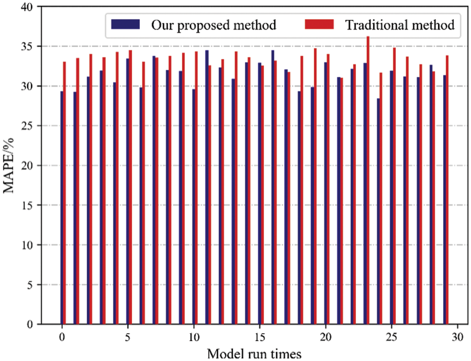
Figure 9: MAPE of EV charging load prediction results under thirty times simulation

From the above analysis results, it can be seen that MAPE of the prediction results by our proposed method is smaller than those by the traditional method twenty-four times, accounting for four-fifths of the total operation times. In most cases, the forecasting effect of our proposed method is better than the traditional method.

The average value of the forecasting load curve of the 30 operation models on January 30 and 31 is shown in Fig. 10. As shown in Fig. 10, it is not difficult to find that the load forecasting results of the proposed method are significantly closer to the real load curve than the traditional load forecasting method. In addition, in the MAPE of the average of 30 forecasting results, the MAPE of the forecasting results of the proposed method is 28.9%, while the MAPE of the traditional method is 33.1%. The forecasting accuracy is improved by nearly 5%, which fully proves the effectiveness of our proposed method.

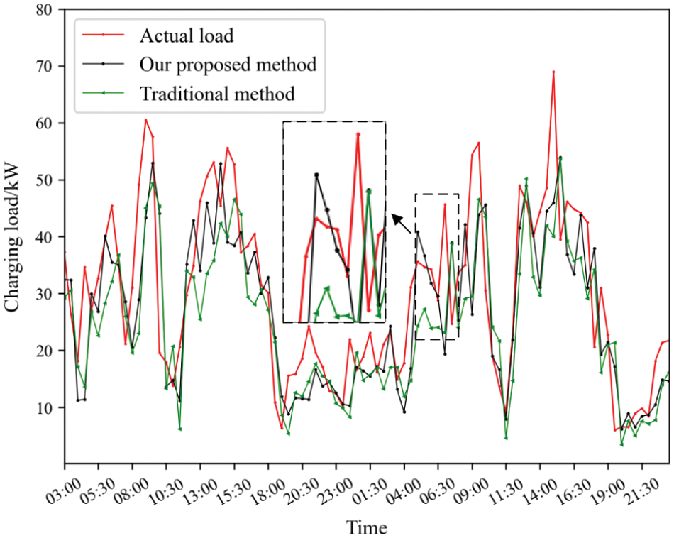
Figure 10: EV charging load forecasting results in 30 and 31 January

3.4.1 Comparison with Different Months

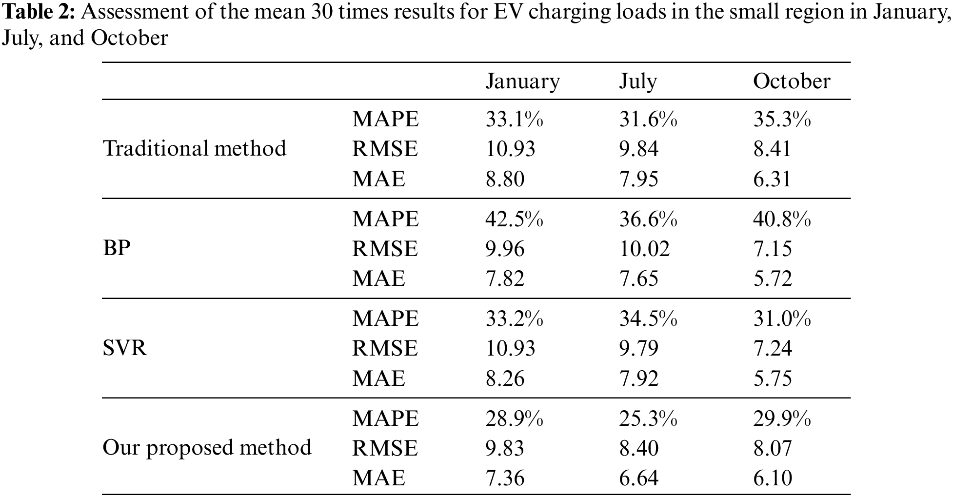
To further verify the validity of the method proposed in this paper, the same method was applied to the regional EV load data for July and October. MAPE for calculating the average of predicted results of 30 times runs in January, July, and October. The results are given in Table 2. It can be found that both the traditional method and our proposed method, the MAPE of July prediction results is the smallest, and the MAPE of October prediction results is the largest.

The prediction results and MAPE for the prediction results in July and October are as shown follow.

The MAPE for the prediction results in July and October are as shown in Fig. 11. It can be seen that MAPE of the prediction results by our proposed method is smaller than those by the traditional method every time in July, and there are only four exceptions in October. In most cases, the forecasting effect of our proposed method is better than the traditional method.

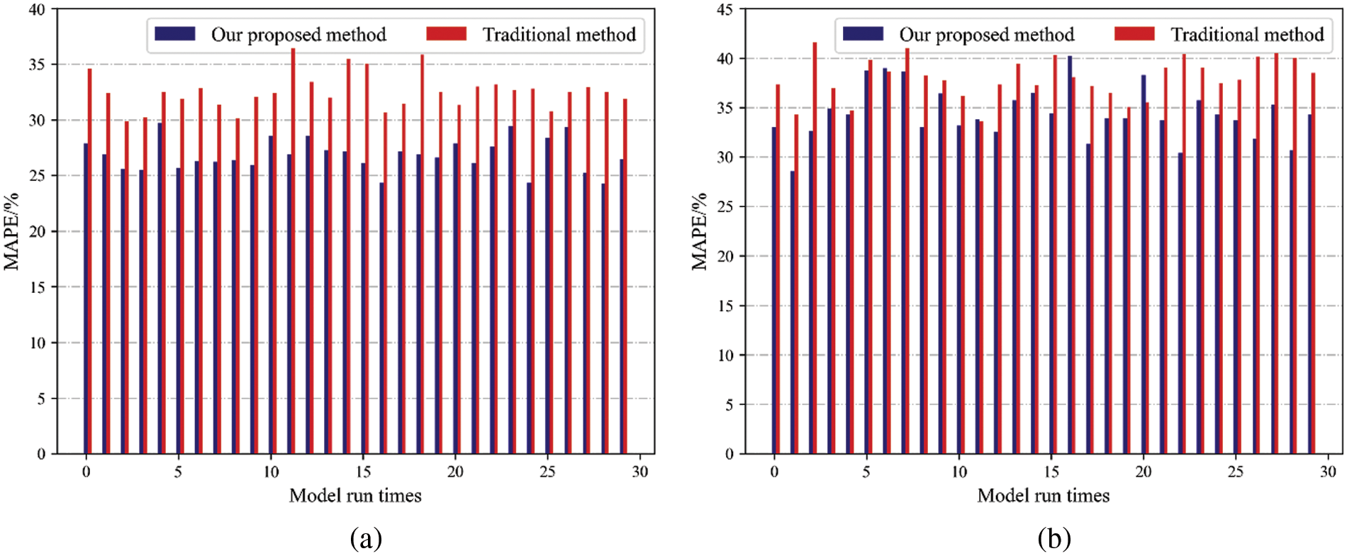
Figure 11: EV charging load prediction errors under thirty times simulation (a) July; (b) October

The average value of the forecasting load curve of the 30 operation models in July and October is shown in Fig. 12. As shown in Fig. 12, it is not difficult to find that the load forecasting results of the proposed method are significantly closer to the real load curve than the traditional load forecasting method.

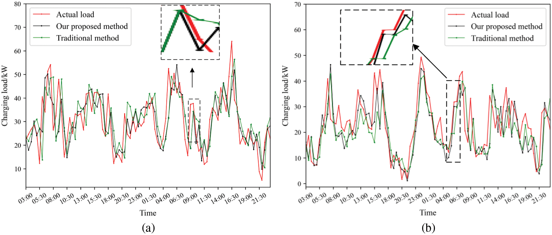
Figure 12: EV charging load forecasting results in (a) 30 and 31 July; (b) 30 and 31 October

For the charging load data of EVs in January, July, and October, the MAPE of the forecasting results of our proposed method is nearly 5% higher than that of the traditional method. The MAPE of the BP forecasting method forecasting results for the small areas in January, July and October are on average about 11% higher than the MAPE of the load forecasting method prediction results in this paper. The MAPE of the forecasting results of the SVR forecasting method for small areas in January, July and October is on average about 5% higher than the MAPE of the forecasting results of the load forecasting method in this paper. The RMSE of the forecasting results of the traditional load forecasting methods for small areas in January, July and October are on average about 1 higher than the RMSE of the forecasting results of the load forecasting methods in this paper. The MAE of the traditional load forecasting method prediction results for small areas in January, July and October are on average about 1.3 higher than the MAE of the load forecasting method forecasting results in this paper. which fully proves the effectiveness of our proposed method.

3.4.2 Comparison with Different Regional Scales

The data used above is the total charging load of 10 charging stations in the small region, the maximum charging load shall not exceed 100 kW. To further verify the validity of the method proposed in this paper, the same method was applied to the regional EV load data for the total charging load of 69 charging stations in the big region.

The prediction results and MAPE for the prediction results in January, July and October in the large region are as shown in Fig. 13.

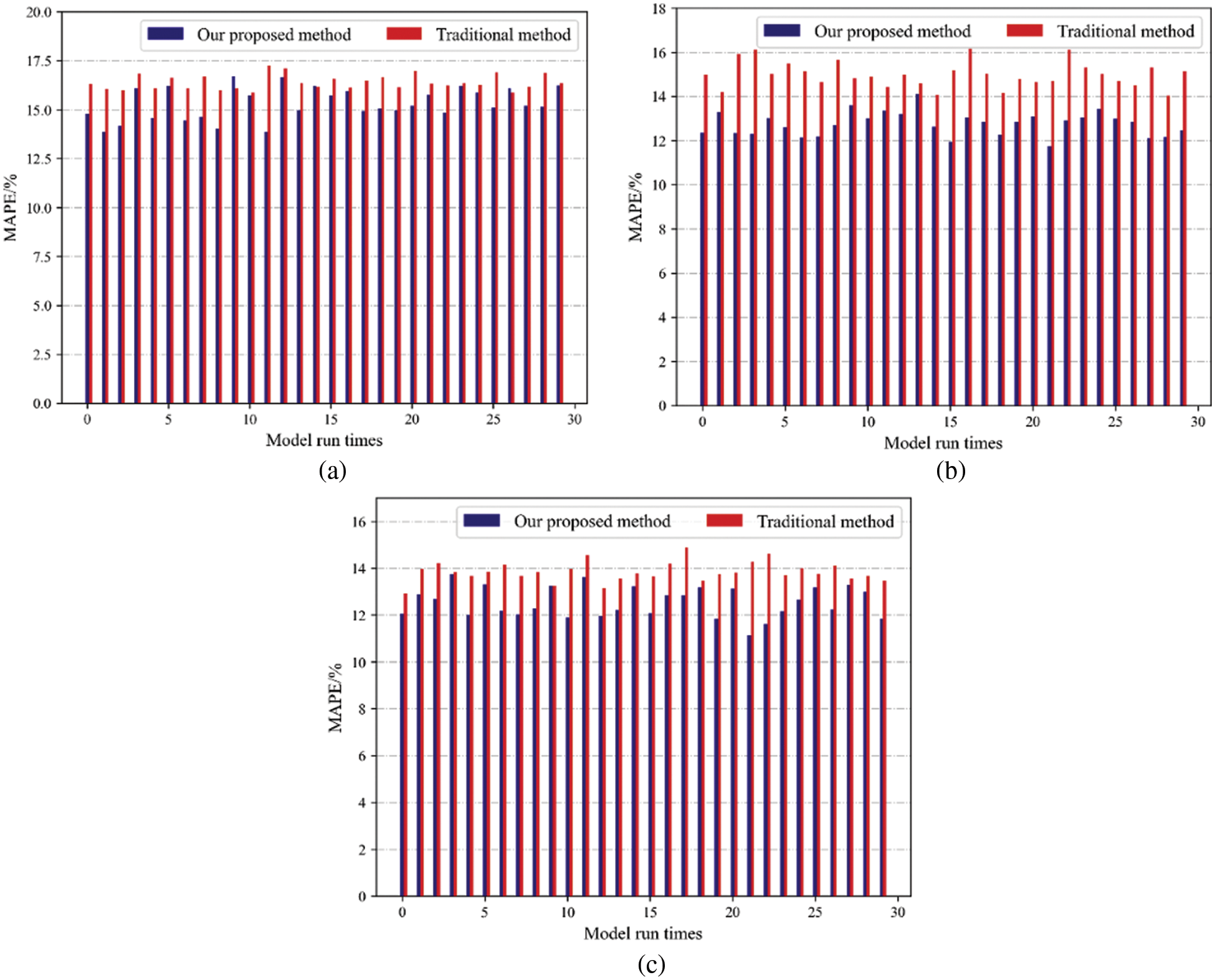
Figure 13: EV load prediction errors under thirty times simulation (a) January; (b) July; (c) October

It can be seen that the MAPE of the prediction results by our proposed method is smaller than those by the traditional method every time in July and October, and there are only three exceptions in January. In most cases, the forecasting effect of our proposed method is better than the traditional method.

The average value of the forecasting load curve of the 30 operation models in January, July and October is shown in Fig. 14. As shown in Fig. 14, it is not difficult to find that the load forecasting results of the proposed method are significantly closer to the real load curve than the traditional load forecasting method.

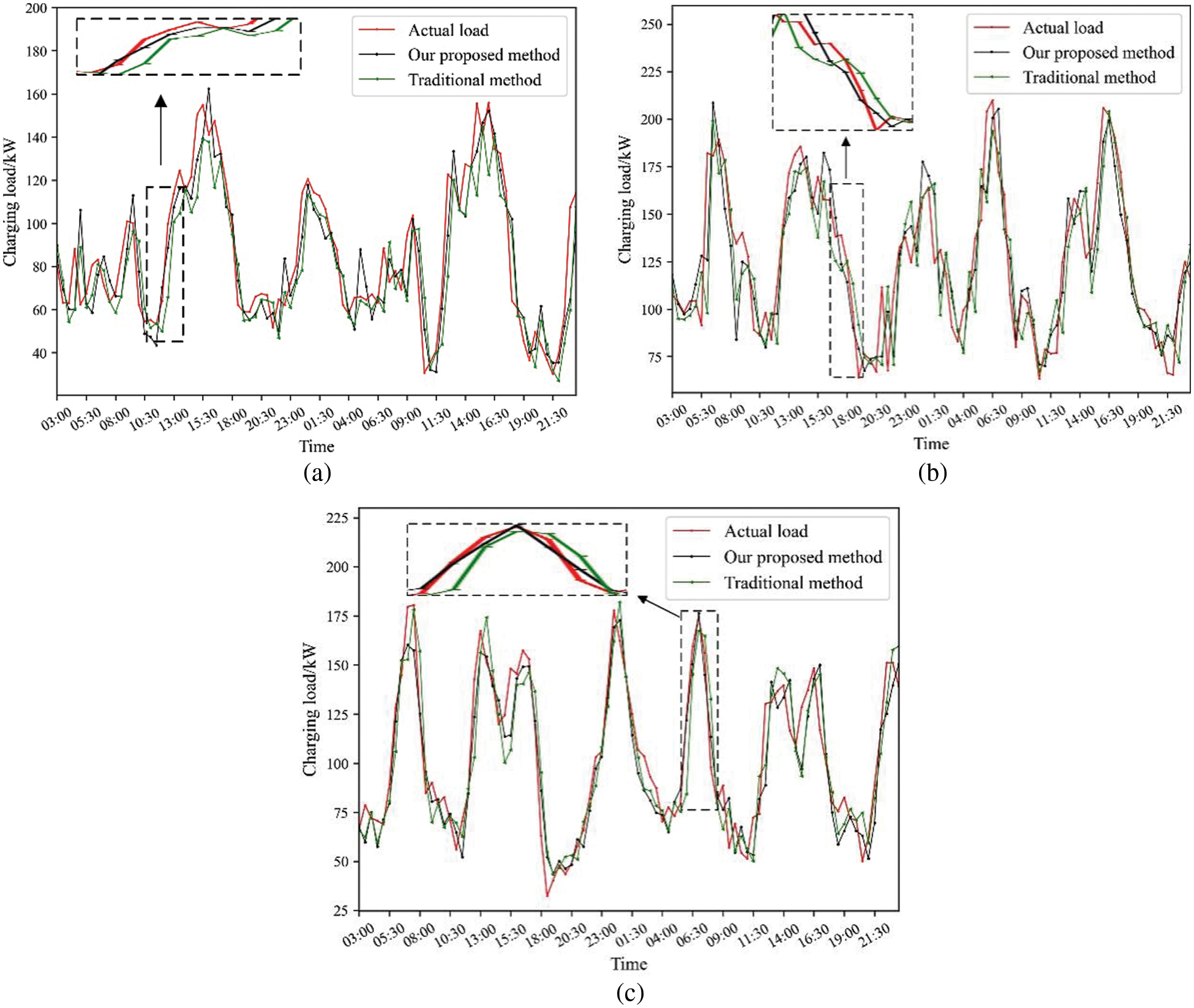
Figure 14: Forecasting results in (a) 30 and 31 January; (b) 30 and 31 July; (c) 30 and 31 October

MAPE for calculating the average of predicted results of 30 times runs in January, July, and October. The results are given in Table 3. It can be found that both the traditional method and our proposed method, the MAPE of October prediction results is the smallest, and the MAPE of January prediction results is the largest.

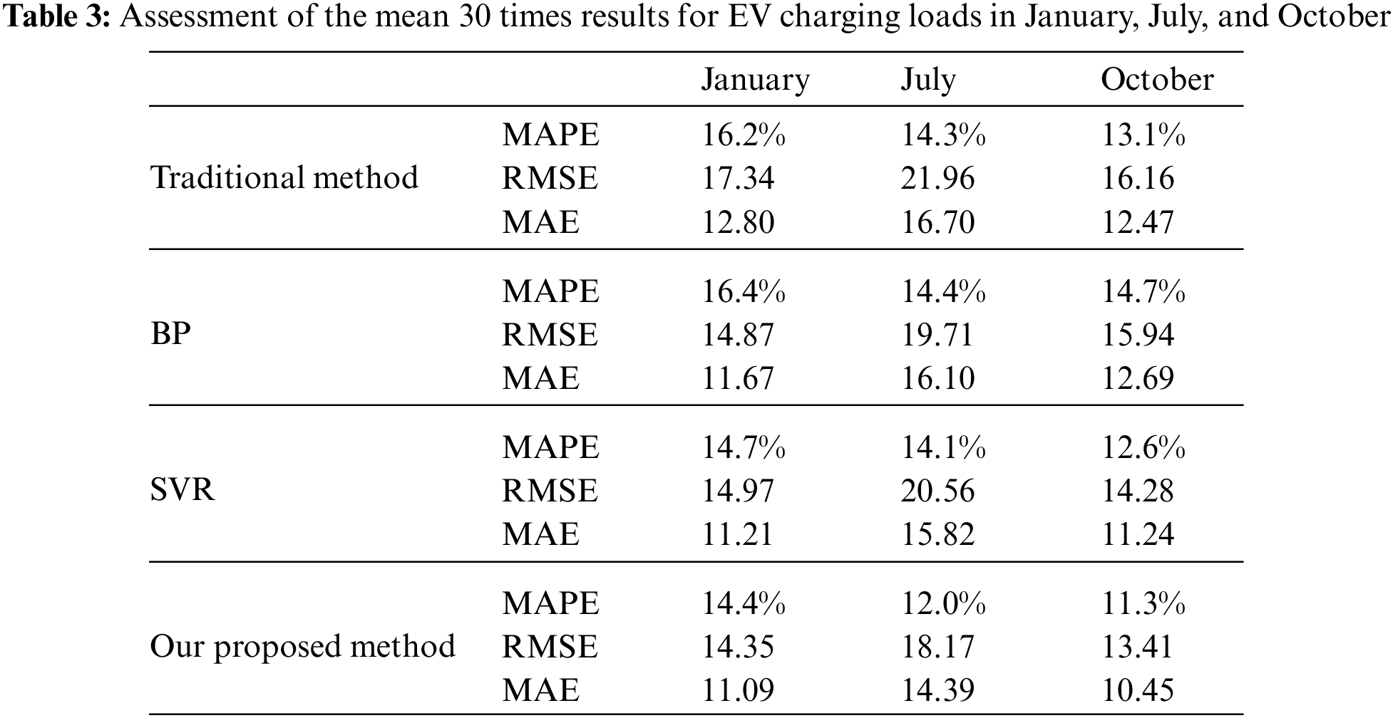
For the charging load data of EVs in January, July, and October, the MAPE of the forecasting results of our proposed method is nearly 2% higher than that of the traditional method. The MAPE of the BP load forecasting method prediction results for large areas in January, July and October are on average about 2.6% higher than the MAPE of the load forecasting method forecasting results in this paper. The MAPE of the forecasting results of the SVR load forecasting method for large regions in January, July and October is on average about 1.2% higher than the MAPE of the forecasting results of the load forecasting method in this paper. The RMSE of the forecasting results of the traditional load forecasting method for large areas in January, July and October are on average about 3 higher than the RMSE of the forecasting results of the load forecasting method in this paper. The MAE of the traditional load forecasting method prediction results for large areas in January, July and October are on average about 1.8 higher than the MAE of the load forecasting method forecasting results in this paper. It can also prove that the forecasting accuracy of forecasting method in this paper is higher than the traditional load forecasting method. It can prove that the forecasting accuracy of forecasting method in this paper is higher than the traditional load forecasting method.

When the results in Table 2 are compared with that in Table 3, we can find that the MAPE of the prediction results in a large region is close to 10%, which is significantly lower than that in a small region, indicating that the larger the charging station is, the more accurate the load prediction can be. The prediction accuracy of total EV charging load of 69 charging stations has achieved great prediction results.

3.5 Load Forecasting Results Assessment

Calculate the load characteristic indexes in Section 2.3, load characteristic indexes and MAPE calculation results are shown in Table 4.

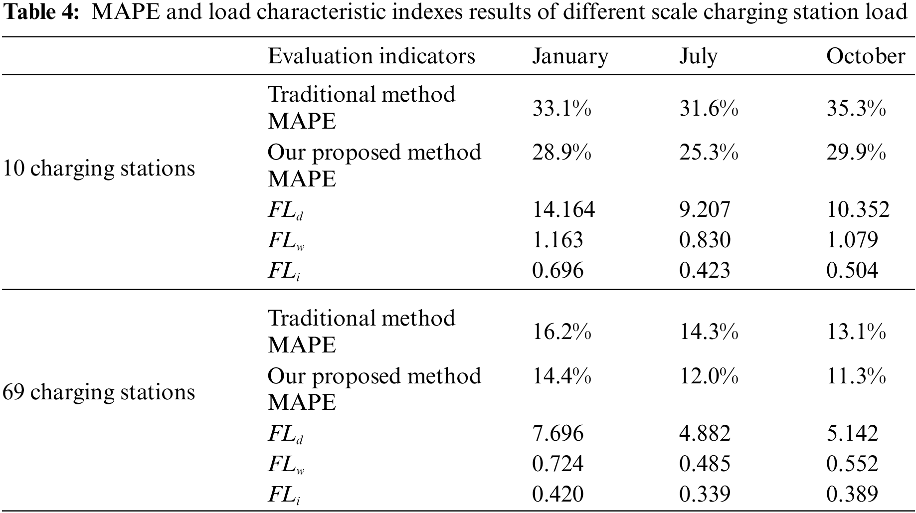
For the total load data of 10 charging stations in a small region, FLi above 0.423, FLd above 7.207, FLw above 0.830, larger values of FLi, FLd, and FLw indicate large fluctuations in the total load of 10 charging stations. For the total load data of 69 charging stations in a large region, FLi below 0.420, it is less than 10 charging stations FLi. FLd below 7.696, FLw below 0.724, compared with FLi of 10 charging stations and 69 charging stations, FLd and FLw of 69 charging stations are significantly smaller than those of 10 charging stations. For the MAPE of the forecasting results of large and small regions, the average MAPE of the forecasting results of a small region is 30%, and the average MAPE of a large region is 12%, with significant differences. FLi obviously does not reflect the difference of load data between large and small regions.

In Fig. 15, the residential load is selected from [32]. The data used are one month of residential load data for different scales of 50 to 200 households. The traditional forecasting method used is the LSTM forecasting model, consistent with the forecasting model used in the traditional method of this paper, The time interval T and the number of days N of the load data are consistent with the data in this paper. The load curves for different types as well as different scales are shown in Fig. 13. Observing Fig. 15, it can be understood that the load amplitude of 150 households is about 75 kW. The same 10 charging stations have a charging load of around 75 kW. It can be seen that the charging load of the 10 charging stations is similar to the load amplitude of 150 households. In the meantime, the adjacent day and adjacent week load fluctuation of residents is slight. In contrast, the charging load law is not obvious, indicating that the charging load has greater volatility than the resident's load. With the same type of load, as the scale increases, adjacent day and adjacent week load volatility have become smaller.

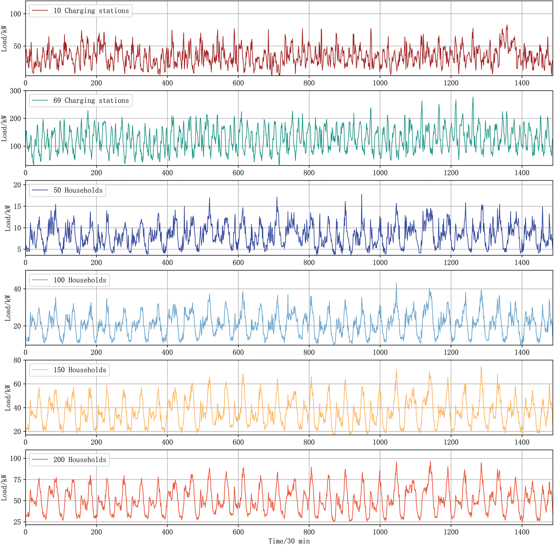
Figure 15: Different type and scaled load curves for residential load and EV charging load

The MAPE and load characteristic indexes of the forecasting results for different types as well as different scales of loads are shown in Table 5.

It can be found that for the same type of load, the larger the scales of the load, the smaller the MAPE of the forecasting result, and the smaller FLd and FLw, while FLi does not show the law. It shows that the larger the scales of the load, the smaller FLd and FLw, the stronger the regularity, and the better the forecasting results can be obtained. FLi has limitations in describing the characteristics of loads at different scales.

The MAPE of load data forecasting results for different types of load data maintains a high positive correlation with FLd and FLw of the data. When the data with higher FLd and FLw are input to the forecasting model, the forecasting result MAPE is larger. FLi of the total load of 69 charging stations is 0.329, FLi for 50 residential loads is 0.320, and the total load of 69 charging stations has a greater FLi but the MAPE of the forecasting results is smaller. FLi for different types of loads cannot show the law that the larger FLi is, the larger the MAPE of the forecasting result is.

In summary, the ability of LSTM load forecasting model to obtain better forecasting results is highly correlated with the load data itself. Data with smaller FLd and FLw are input to the forecasting model, and better forecasting results are obtained. A single FLi does not have the feature of accurately determining the magnitude of MAPE of load data forecasting results before forecasting. FLd and FLw proposed in this paper can well depict the regularity and the strength of volatility of the load data, and the calculated results can maintain a high correlation with MAPE of load data forecasting results, which can be effectively used to determine the MAPE size of the forecasting result before forecasting.

4  Conclusions

To improve the ultra short-term predication accuracy of EV charging load, EV charging pile usage degree is defined by us based on the usage frequency of charging piles. And then the EV charging pile usage degree data is merged with the historical charging load data as the input variables in the LSTM-based ultra short-term forecasting model.

Simulation results show that the larger the maximum power of the historical load data is, the higher the load forecasting accuracy is. FLd and FLw proposed in this paper can well depict the regularity and the strength of volatility of the load data, and the calculated results can maintain a high correlation with MAPE of load data forecasting results. The EV charging load data used in this paper have greater FLd and FLw, which also indicates that the EV charging load has greater adjacent day and adjacent week volatility relative to the residential load, making it more difficult to forecasting.

The simulation results show that when the charging load data FLd is about 11.241 and FLw is about 1.024, the MAPE of the traditional load forecasting method is about 33.3%, the MAPE of the BP load forecasting method is about 40.0%, the MAPE of the SVR load forecasting method is about 32.9%, and the MAPE of the forecasting method in our proposed is about 28%. When the charging load data FLd is about 5.907 and FLw is 0.587, the MAPE of the traditional load forecasting method is about 14.5%, the MAPE of the BP load forecasting method is about 15.2%, the MAPE of the SVR load forecasting method is about 13.8%, and the MAPE of the forecasting method in our proposed is about 12.6%. It can be seen that for different categories of data, the forecasting effect of the method proposed in this paper is always better than the traditional various load forecasting methods, and secondly, the load volatility indexes FLd and FLw proposed in this paper can well respond to the volatility of the load data, and can judge whether the load data can have a better forecasting effect before forecasting.

Funding Statement: This work is supported by National Key R&D Program of China (No. 2021YFB2601602).

Conflicts of Interest: The authors declare that they have no conflicts of interest to report regarding the present study.

References

1. Zhou, X., Zou, S. L., Wang, P., Ma, Z. J. (2021). ADMM-based coordination of electric vehicles in constrained distribution networks considering fast charging and degradation. IEEE Transactions on Intelligent Transportation Systems, 22(1), 565–578. DOI 10.1109/TITS.2020.3015122. [Google Scholar] [CrossRef]
2. Wang, J., Bharati, G. R., Paudyal, S., Ceylan, O., Bhattarai, B. P. et al. (2019). Coordinated electric vehicle charging with reactive power support to distribution grids. IEEE Transactions on Industrial Informatics, 15(1), 54–63. DOI 10.1109/TII.2018.2829710. [Google Scholar] [CrossRef]
3. Hoverstad, B. A., Tidemann, A., Langseth, H., Ozturk, P. (2015). Short-term load forecasting with seasonal decomposition using evolution for parameter tuning. IEEE Transactions on Smart Grid, 6(4), 1904–1913. DOI 10.1109/TSG.2015.2395822. [Google Scholar] [CrossRef]
4. Jiang, M., Gu, D. J., Kong, J., Tian, Y. Z. (2018). Short-term load forecasting model based on online sequential extreme support vector regression. Power System Technology, 42, 2240–2247. [Google Scholar]
5. Zhang, S. Y., Leung, K. C. (2022). Joint optimal power flow routing and vehicle-to-grid scheduling: Theory and algorithms. IEEE Transactions on Intelligent Transportation Systems, 23(1), 499–512. DOI 10.1109/TITS.2020.3012489. [Google Scholar] [CrossRef]
6. Deng, D. Y., Li, J., Zhang, Z. Y., Teng, Y. F., Huang, Q. (2020). Short-term electric load forecasting based on EEMD-GRU-MLR. Power System Technology, 44, 593–602. [Google Scholar]
7. Amral, N., Ozveren, C. S., King, D. (2007). Short term load forecasting using multiple linear regression. Universities Power Engineering Conference, pp. 1192–1198. Brighton, UK. [Google Scholar]
8. Li, W., Zhang, Z. G. (2009). Based on time sequence of ARIMA model in the application of short-term electricity load forecasting. Proceedings of the 2009 International Conference on Research Challenges in Computer Science, pp. 11–14. Shanghai, China. [Google Scholar]
9. Shankar, R., Chatterjee, K., Chatterjee, T. (2015). A very short-term Load forecasting using kalman filter for load frequency control with economic load dispatch. Journal of Engineering Science and Technology Review, 5, 97–103. [Google Scholar]
10. Quan, H., Srinivasan, D., Khosravi, A. (2014). Short-term load and wind power forecasting using neural network-based prediction intervals. IEEE Transactions on Neural Networks & Learning Systems, 25(2), 303–315. DOI 10.1109/TNNLS.2013.2276053. [Google Scholar] [CrossRef]
11. Park, D. C., El-Sharkawi, M. A., Marks, R. J., Atlas, L. E., Damborg, M. J. (1991). Electric load forecasting using an artificial neural network. IEEE Transactions on Power Systems, 6(2), 442–449. DOI 10.1109/59.76685. [Google Scholar] [CrossRef]
12. Chen, B. J., Chang, M. W., Lin, C. J. (2004). Load forecasting using support vector machines. IEEE Transactions on Power Systems, 19(4), 1821–1830. DOI 10.1109/TPWRS.2004.835679. [Google Scholar] [CrossRef]
13. Ko, C. N., Lee, C. M. (2013). Short-term load forecasting using SVR (support vector regression)-based radial basis function neural network with dual extended kalman filter. Energy, 49(12), 413–422. DOI 10.1016/j.energy.2012.11.015. [Google Scholar] [CrossRef]
14. Fan, G. F., Peng, L. L., Hong, W. C., Sun, F. (2016). Electric load forecasting by the SVR model with differential empirical mode decomposition and auto regression. Neurocomputing, 173, 958–970. DOI 10.1016/j.neucom.2015.08.051. [Google Scholar] [CrossRef]
15. Hinton, G. E., Osindero, S., Teh, Y. W. (2006). A fast learning algorithm for deep belief nets. Neural Computation, 18(7), 1527–1554. DOI 10.1162/neco.2006.18.7.1527. [Google Scholar] [CrossRef]
16. Cao, F., Li, S., Zhang, Y. (2021). Temporal and spatial distribution simulation of EV charging load considering charging station attractiveness. Power System Technology, 45, 75–87. [Google Scholar]
17. Gilanifar, M., Parvania, M. (2021). Clustered multi-node learning of electric vehicle charging flexibility. Applied Energy, 282(28), 116125. DOI 10.1016/j.apenergy.2020.116125. [Google Scholar] [CrossRef]
18. Zhao, Y., Wang, Z. P., Shen, Z. J. M., Sun, F. C. (2021). Data-driven framework for large-scale prediction of charging energy in electric vehicles. Applied Energy, 282, 116175. DOI 10.1016/j.apenergy.2020.116175. [Google Scholar] [CrossRef]
19. Jiang, Z. Z., Xiang, Y., Liu, J. Y., Zhu, J. Y., Shui, Y. (2019). Charging load modeling integrated with electric vehicle whole trajectory space and its impact on distribution network reliability. Power System Technology, 43, 3789–3800. [Google Scholar]
20. Wang, H. L., Zhang, M. X., Yang, X. (2017). Electric vehicle charging demand forecasting based on influence of weather and temperature. Electrical Measurement & Instrumentation, 54, 123–128. [Google Scholar]
21. Dabbaghjamanesh, M., Moeini, A., Kavousi-Fard, A. (2021). Reinforcement learning-based load forecasting of electric vehicle charging station using q-learning technique. IEEE Transactions on Industrial Informatics, 17(6), 4229–4237. DOI 10.1109/TII.2020.2990397. [Google Scholar] [CrossRef]
22. Bae, S., Kwasinski, A. (2012). Spatialand temporal model of electric vehicle charging demand. IEEE Transaction on Smart Grid, 3(1), 394–403. DOI 10.1109/TSG.2011.2159278. [Google Scholar] [CrossRef]
23. Bashash, S., Fathy, H. K. (2012). Transport-based load modeling and sliding mode control of plug-in electric vehicles for robust renewable power tracking. IEEE Transactions on Smart Grid, 3(1), 526–534. DOI 10.1109/TSG.2011.2167526. [Google Scholar] [CrossRef]
24. Niri, M. F., Dinh, T. Q., Yu, T. F., Marco, J., Bui, T. M. N. (2021). State of power prediction for lithium-ion batteries in electric vehicles via wavelet-markov load analysis. IEEE Transactions on Intelligent Transportation Systems, 22(9), 5833–5848. DOI 10.1109/TITS.2020.3028024. [Google Scholar] [CrossRef]
25. Zhu, J. C., Yang, Z. L., Guo, Y. J., Zhang, J. K., Yang, H. K. (2019). Short-term load forecasting for electric vehicle charging stations based on deep learning approaches. Applied Sciences, 9(9), 2076–3417. DOI 10.3390/app9091723. [Google Scholar] [CrossRef]
26. Liu, Y. X., Zhang, N., Kang, C. Q. (2018). A review on data-driven analysis and optimization of power grid. Automation of Electric Power Systems, 42, 157–167. [Google Scholar]
27. Barman, M., Choudhury, N. B. D., Sutradhar, S. (2017). A regional hybrid GOA-SVM model based on similar day approach for short-term load forecasting in Assam. Energy, 145, 710–720. DOI 10.1016/j.energy.2017.12.156. [Google Scholar] [CrossRef]
28. Lin, W. X., Wu, D., Boulet, B. (2021). Spatial-temporal residential short-term load forecasting via graph neural networks. IEEE Transactions on Smart Grid, 12(6), 5373–5384. DOI 10.1109/TSG.2021.3093515. [Google Scholar] [CrossRef]
29. Wen, L. L., Zhou, K. L., Yang, S. L. (2019). Load demand forecasting of residential buildings using a deep learning model. Electric Power Systems Research, 179, 106073. DOI 10.1016/j.epsr.2019.106073. [Google Scholar] [CrossRef]
30. Zang, H. X., Xu, R. Q., Chen, L. L., Ding, T., Liu, L. et al. (2021). Residential load forecasting based on LSTM fusing self-attention mechanism with pooling. Energy, 229(1), 120682. DOI 10.1016/j.energy.2021.120682. [Google Scholar] [CrossRef]
31. Kong, W. C., Dong, Z. Y., Jia, Y. W., Hill, D. J., Xu, Y. et al. (2019). Short-term residential load forecasting based on LSTM recurrent neural network. IEEE Transactions on Smart Grid, 10(1), 841–851. DOI 10.1109/TSG.2017.2753802. [Google Scholar] [CrossRef]
32. Hou, T. T., Fang, R. R., Tang, J. R., Ge, G. H., Yang, D. J. et al. (2021). A novel short-term residential electric load forecasting method based on adaptive load aggregation and deep learning algorithms. Energies, 14(22), 7820. DOI 10.3390/en14227820. [Google Scholar] [CrossRef]
Cite This Article
Copyright © 2023 The Author(s). Published by Tech Science Press.
This work is licensed under a Creative Commons Attribution 4.0 International License , which permits unrestricted use, distribution, and reproduction in any medium, provided the original work is properly cited.
Downloads
Citation Tools