
 Submit a Paper
 Propose a Special lssue
 Open Access
ARTICLE
Experimental Study on the Performance of ORC System Based on Ultra-Low Temperature Heat Sources
1 College of Mechanical Engineering, Tianjin University of Science & Technology, Tianjin, 300222, China
2 School of Energy Engineering, Tianjin Sino-German University of Applied Sciences, Tianjin, 300350, China
3 Tianjin “The Belt and Road” Joint Laboratory, Tianjin Sino-German University of Applied Sciences, Tianjin, 300350, China
* Corresponding Author: Lian Zhang. Email:
Energy Engineering 2024, 121(1), 145-168. https://doi.org/10.32604/ee.2023.042798
Received 12 June 2023; Accepted 01 September 2023; Issue published 27 December 2023
 View Full Text
 Download PDF
Abstract
This paper discussed the experimental results of the performance of an organic Rankine cycle (ORC) system with an ultra-low temperature heat source. The low boiling point working medium R134a was adopted in the system. The simulated heat source temperature (SHST) in this work was set from 39.51°C to 48.60°C by the simulated heat source module. The influence of load percentage of simulated heat source (LPSHS) between 50% and 70%, the rotary valve opening (RVO) between 20% and 100%, the resistive load between 36 Ω and 180 Ω or the no-load of the generator, as well as the autumn and winter ambient temperature on the system performance were studied. The results showed that the stability of the system was promoted when the generator had a resistive load. The power generation (PG) and generator speed (GS) of the system in autumn were better than in winter, but the expander pressure ratio (EPR) was lower than in winter. Keep RVO unchanged, the SHST, the mass flow rate (MFR) of the working medium, GS, and the PG of the system increased with the increasing of LPSHS for different generator resistance load values. When the RVO was 60%, LPSHS was 70%, the SHST was 44.15°C and the resistive load was 72 Ω, the highest PG reached 15.11 W. Finally, a simulation formula was obtained for LPSHS, resistance load, and PG, and its correlation coefficient was between 0.9818 and 0.9901. The formula can accurately predict the PG. The experimental results showed that the standard deviation between the experimental and simulated values was below 0.0792, and the relative error was within ±5%.Keywords
Nomenclature
| Symbols | |
| Mass flow rate, | |
| Fan air volume, | |
| Density, | |
| Specific heat capacity, | |
| Temperature, | |
| Enthalpy, | |
| Pressure, | |
| Power, | |
| Voltage, | |
| Current, | |
| Speed, | |
| Abbreviation | |
| ORC | Organic Rankine cycle |
| RVO | Rotary valve opening |
| SHST | Simulated heat source temperature |
| LPSHS | Load percentage of simulated heat source |
| MFR | Mass flow rate |
| GS | Generator speed |
| PG | Power generation |
| EPR | Expander pressure ratio |
| Subscripts | |
| cond | Condenser |
| gen | Generator |
| exp | Expander |
| eva | Evaporator |
| in | Inlet |
| out | Outlet |
The extensive utilization of fossil energy has led to serious environmental problems [1], such as the greenhouse effect, haze, acid rain, etc. ORC technology utilizes industrial waste heat, geothermal energy, and solar thermal energy as heat sources for power generation [2–4]. The use of ORC technology improves energy efficiency and reduces carbon emissions to the environment.
In terms of system cost and carbon emission, Calli et al. [5] studied the power demand of a farm and found that the cost-benefit ratio of using both the ORC system and the power grid was 30% higher than using the power grid alone. Köse et al. [6] found that the economics of the Kalina cycle was 3.93 years better than that of the ORC cycle, but the ORC cycle was superior to the Kalina cycle in terms of energy, exergy, and CO2 reduction. Regarding the working fluid and lubricating oil of the system, Hijriawan et al. [7] studied the performance of R134a in an ORC system. The results showed that when the scroll expander speed was 505.8 RPM and the system power was 584.5 W, the energy efficiency of the system was up to 3.17%. Yang et al. [8] studied the effect of lubricating oil ratio in an ORC system. The results showed that the maximum thermal efficiency of the system was 4.7% at a high oil ratio. Regarding the type of heat source, Chen et al. [9] used a solar-assisted ORC system and showed that solar energy not only improves heat recovery efficiency but also reduces annual total cost. Ma et al. [10] proposed an efficient integrated energy system to recover waste heat from power plants. It was concluded that when the MFR of the exhaust gas was adjusted to 70 kg/s, the PG was 7500 kW. Loni et al. [11] reviewed and discussed the operation methods of geothermal-driven ORC systems. It showed that the performance of the geothermal-driven ORC system can be improved by 20% to 30% after optimization. When it comes to waste heat utilization, Sleiti et al. [12] studied the performance of the TMR system under waste heat conditions ranging from 50°C to 85°C. Although this research was of great significance in the low-temperature field, there has been no research on waste heat below 50°C. Pan et al. [13] proposed an ORC system for waste incineration energy recovery. The results showed that the energy efficiency, the exergy efficiency, and the ecological efficiency of the system increased to 41.22%, 66.91%, and 84.54%, respectively. Varis et al. [14] recovered the waste heat generated by 26 gas engines in a certain area. They tested the exhaust gas flow, temperature, and pressure values at the chimney outlet of the engine to obtain the best consumption value and the optimal mechanical power of the equipment in the ORC system. Peng et al. [15] used the heat extracted from coal gangue to generate electricity. They studied the arrangement mode, hierarchical structure, and cold-end heat dissipation mode of the thermoelectric module and proposed a thermoelectric conversion structure that reduced heat loss and improved the output power of thermoelectric conversion. In relation to cross-seasonal environmental conditions, Wang et al. [16] studied the cross-seasonal performance of the ORC system under variable condensation conditions. They found that when the wet bulb temperature was 1.1°C, the power generation and PG efficiency of the system reached 8.04 kW and 11.31%, respectively. Concerning the component equipment of the system, Han et al. [17] used a five-cylinder radial piston expander to recover waste heat for PG. By adjusting the pump speed, the output power of the expander can be optimized, with a total thermal efficiency of 2.02% and a firing efficiency of 10.5% respectively. Wu et al. [18] used a radial inflow turbine generator to study the performance of the ORC system and tested its performance under different speeds, turbine inlet temperatures, and generator loads. The results showed that when the generator reached the rated speed, the output power was 20.47 kW and PG efficiency was 91.1%, respectively. Wu et al. [19] studied the performance of the OR system using a high-speed radial inflow turbine and tested the system performance under different load powers. The results showed that the PG and thermal efficiency of the system were 1.424 kW and 2.52%, respectively. By using a free-piston expander linear generator, Yang et al. [20] studied the performance of the ORC system and found that the maximum energy conversion efficiency of the system was 28.81% when the expander inlet pressure was 0.2 MPa, the operating frequency was 1.5 Hz and the resistive load was 5 Ω. Chen et al. [21] used a model that integrated thermal power generation, computational fluid dynamics, and plate fins to study the ORC system. The results showed that when there were no baffles in the individual module, it could provide accurate prediction results for the system. Zhou et al. [22] used the waste heat generated by wind turbines in a poly-generation system, filling the gap in the waste heat utilization of generators. Shoeibi et al. [23] introduced an improved single-slope solar evaporator to enhance evaporation efficiency, increasing it by 7 W/h compared to traditional solar evaporators. Kaczmarczyk et al. [24] investigated the performance of the 1 kWe scroll expander in an ORC system. The results showed that the maximum efficiency of the expander was 49.31%, and the thermal and exergy efficiency of the cycle were 5.97% and 15.82%, respectively. For the system workload, Cao et al. [25] studied the steady-state and transient performance of the ORC system by using the lamp array to simulate variable external loads. The steady-state showed that the system efficiency reached its maximum when the resistive load was smaller than the ORC power capacity at 50 Hz frequency. The transient analysis showed that the resistive load and the parameters of the heat source had little effect on the electrical quality. Jin et al. [26] studied the influence of resistive load on system performance using a 3 kW ORC system. The results showed that when the resistive load was constant, the increase in power generation of the system led to an increase in the speed and inlet pressure of the expander. Kaczmarczyk et al. [27] simulated the heat source power of the household boiler (12–20 kW), adjusted the rated power of the generator load (200–2000 W), and carried out experimental research on a 1 kW high-speed ORC micro-disturbance generator, the overcompensation and under compensation intervals of the synchronous generator were obtained under different load levels. The results showed that when the load current of the micro-disturbance generator was optimal, the PG was higher.
However, the above research focuses mainly on the influence of the type of working medium and heat source, the components of the system, and the resistive load of the generator in the ORC system. There is little research on the ultra-low temperature performance of the ORC system, particularly the performance below 50°C. The research on ultra-low temperature heat sources will fill the gap in ultra-low temperature ORC power generation systems. The working medium used in the system was R134 a, and the simulated heat source module was established. The effects of LPSHS (50%–70%), RVO (20%–100%), the resistive load of the generator (36–180 Ω or no load), and the ambient temperature in autumn and winter on the system performance were studied. Furthermore, the novelty and originality of the paper are highlighted. Experimental formulas relating to LPSHS, resistive load, and PG are fitted based on the collected experimental data. According to this formula, the PG can be accurately predicted, providing theoretical and practical guidance for the intelligent control of the PG of the system. In addition, through literature research, it was found that there is little use of low-temperature thermal power generation systems for experimental teaching. Therefore, this experimental system has the advantages of a stable heat source, low heat source temperature, small equipment size, and easy transportation, which will be beneficial for teachers’ experimental teaching. Through teaching, students can master the theoretical and experimental knowledge of low-temperature thermoelectric power generation systems and enhance their awareness of energy conservation.
In order to study the performance of the ORC system with ultra-low temperature heat source, a corresponding experimental platform was built with R134a as the working medium. The schematic diagram of this experimental platform is shown in Fig. 1, and its main equipment included: air-cooled evaporator (1), simulated heat source module (2), expander (3), DC generator (6) and its resistive load (7), air-coiled condenser (4), rotational valve (5), etc. The resistive load was referred to as a range of 36–180 Ω between 3, 5, 7, 9 Ω [20] and 200–2000 W [27] as the range of resistive in this study. The main equipment parameters of the system are shown in Table 1.
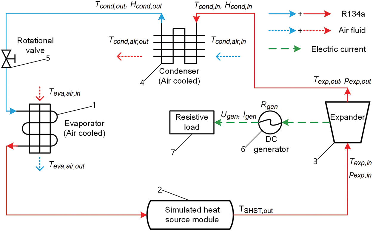
Figure 1: System schematic diagram
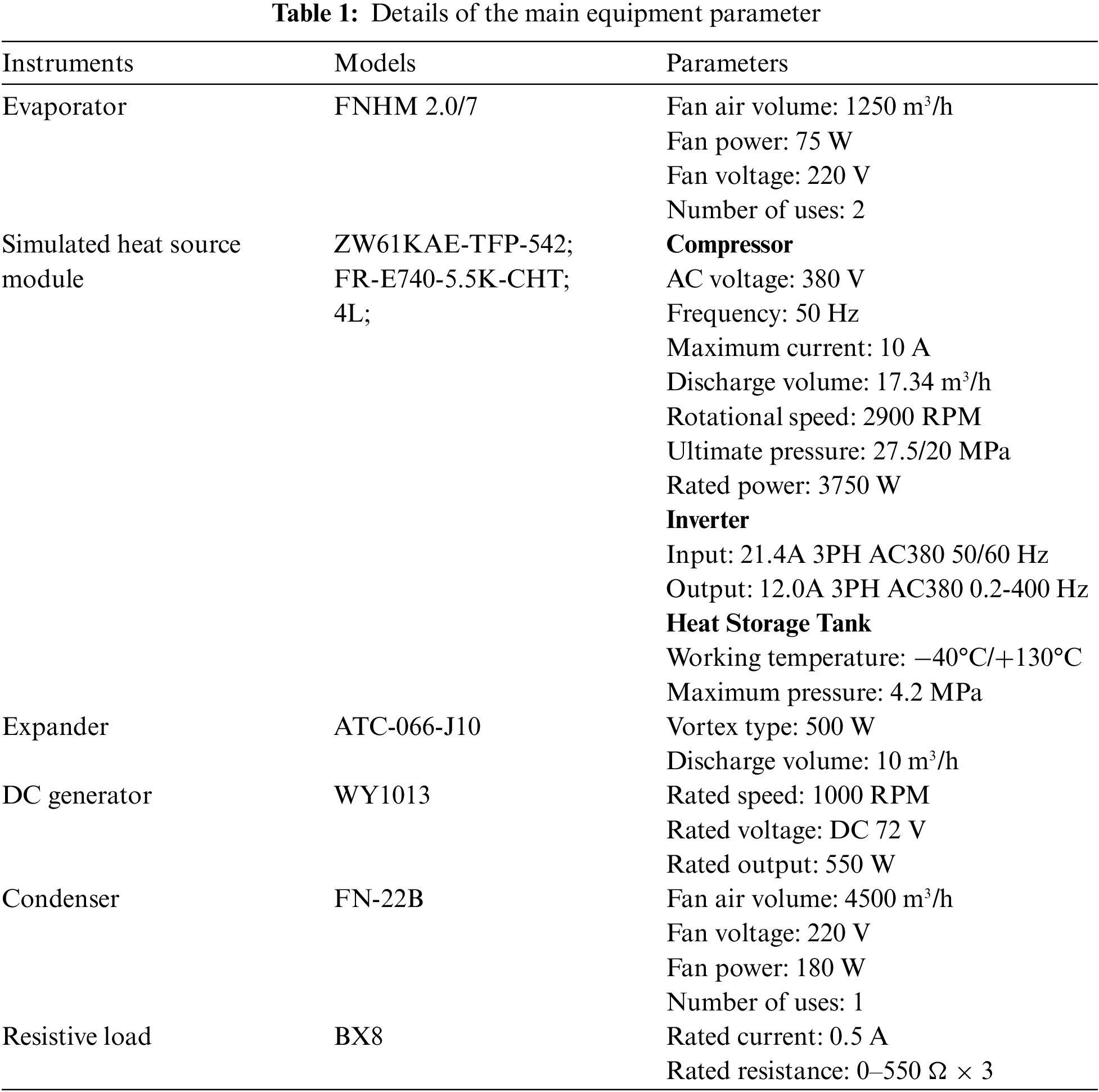
Fig. 2 shows the physical diagram of the system, the simulated heat source module included: an inverter (2c), compressor (2a) and heat storage tank (2b), etc.
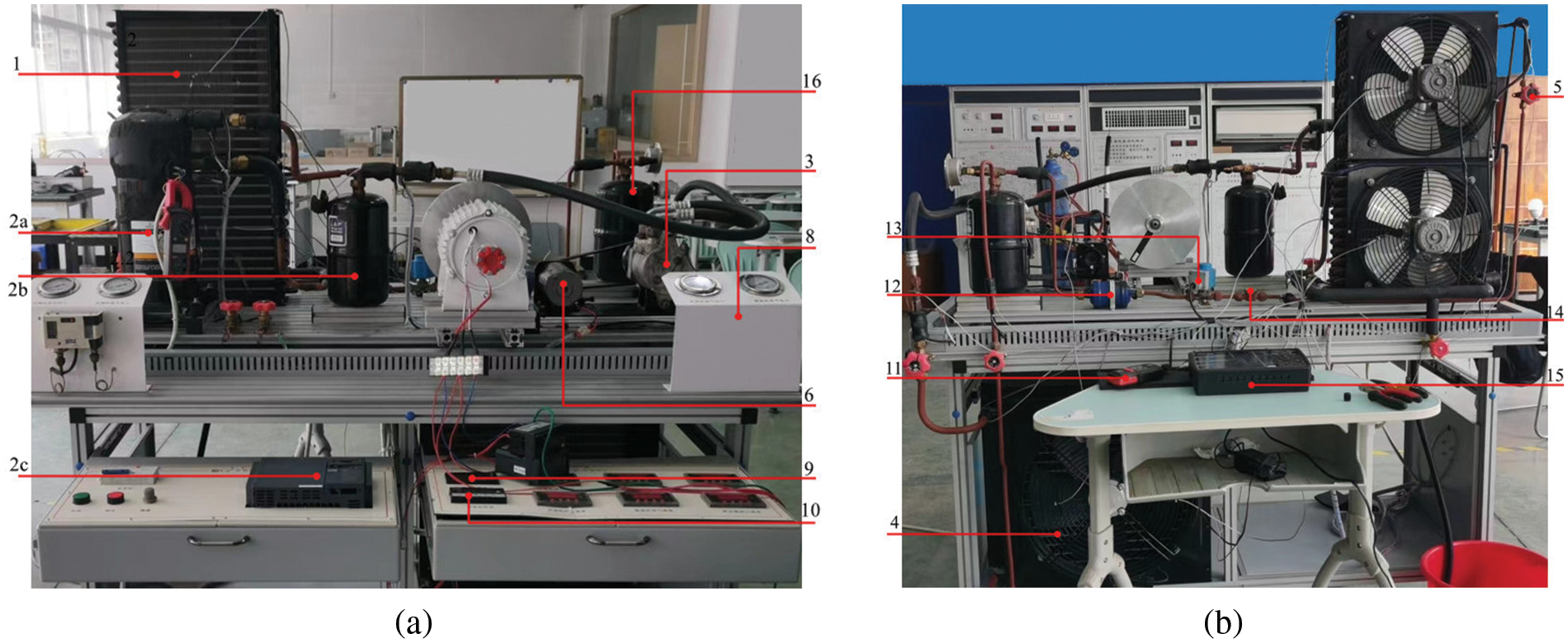
Figure 2: Physical diagrams of system (a) Front view, (b) Rear view, 1-Air coiled evaporator, 2a-Compressor, 2b-Heat storage tank, 2c-Inverter, 3-Expansion, 4-Air coiled condenser, 5-Rotational valve, 6-DC generator, 7-Resistive load, 8-Pressure gauge, 9-DC voltmeter, 10-DC ammeter, 11-Speed Indicator, 12-Filter, 13-Solenoid valve, 14-Visual liquid mirror, 15-Data acquisition instruments, 16-Liquid storage tank
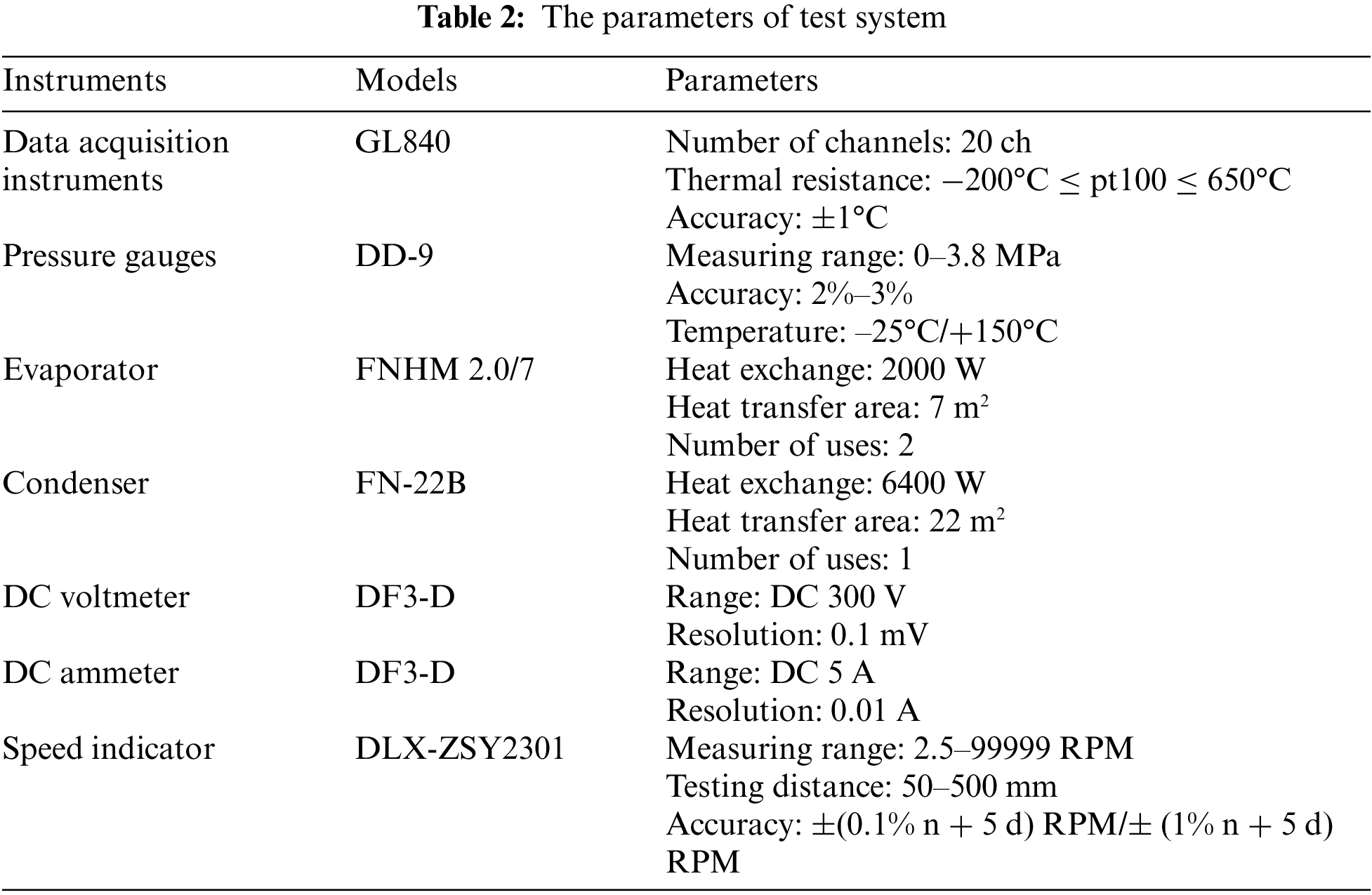
During the operation of the system, the heat supply of the simulated heat source module (2) was changed by adjusting the frequency of the compressor (2a). The rated power of the simulated heat source module was 3750 W, which meant the LPSHS was 100 %. The SHST and MFR of the working medium were affected by the LPSHS. After passing through the simulated heat source module, the working medium enters the expander (3), which drives the generator (6) to generate electricity. The working medium came out of the expander and entered the air-coiled condenser (4), where the air acted as a cooling source to cool the working medium passing through the condenser. The working medium flowed out of the condenser and entered the air-coiled evaporator (1) through the rotational valve, where the air preheated the working medium through the evaporator. The preheated working medium flowed into the simulated heat source module. The performance of the ORC system was studied by adjusting the resistive load (7) of the generator, the RVO, and the LPSHS. Table 2 shows the parameters of the test system.
The mass flow rate of R134a in the condenser can be expressed as in Eq (1).
The power generated by the generator can be expressed as in Eq (2).
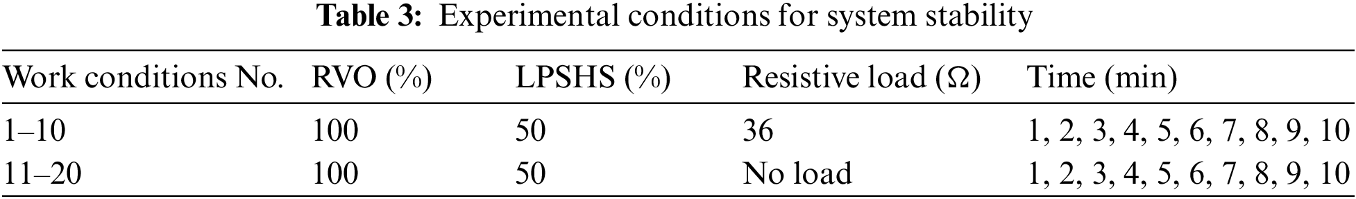
In this paper, different working conditions were studied in detail. For working conditions No. 1–20, the working medium of the system was R134a, the room temperature was kept at 21°C by adjusting the central air conditioner, RVO was set to 100%, LPSHS was set to 50%, and the resistive load of the generator was set as 36 Ω or no load. In order to study the stability of the system, the changes in the inlet temperature and pressure of the expander were detected within 10 min of the system operation, as shown in Table 3.
3.2.2 System Variations under Generator No-Load
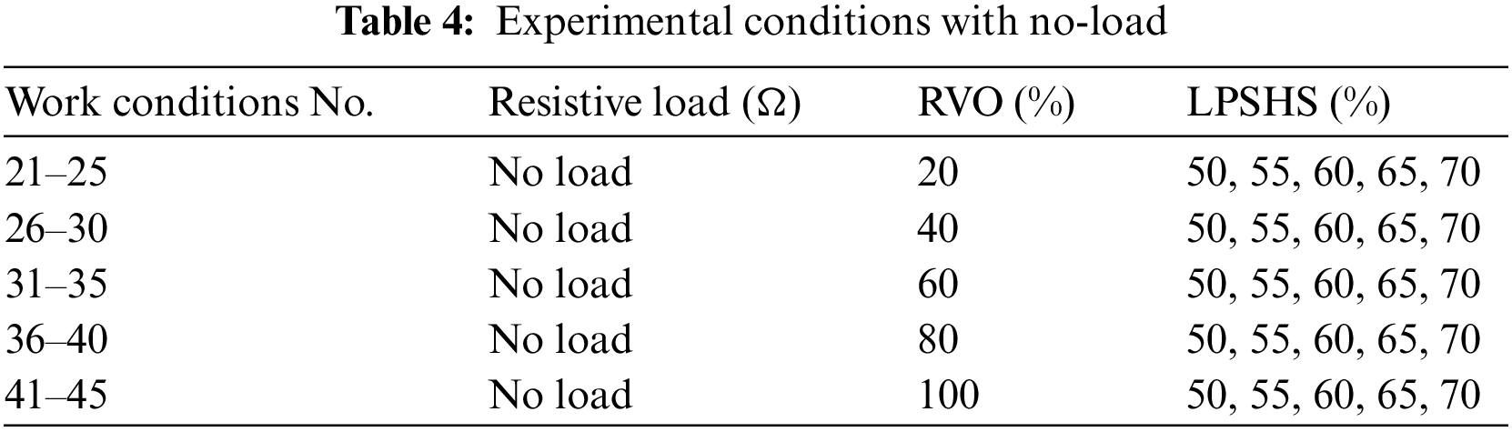
For working conditions No. 21–45, the system used R134a, the central air conditioner was adjusted to keep the room temperature at 21°C, the RVO was 20%–100%, the LPSHS was 50%–70%, and the generator with no-load, as shown in Table 4.
3.2.3 System Variations under Generator Load
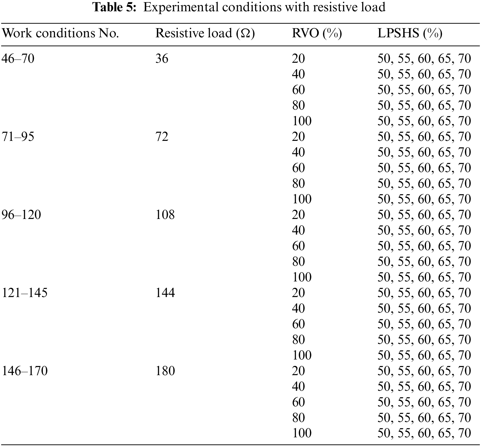
For working conditions No. 46–170, the system used R134a, the central air conditioner was adjusted to keep the room temperature at 21°C, the RVO was 20%–100%, the LPSHS was 50%–70%, and the resistive load of the generator was 36–180 Ω, as shown in Table 5.
3.2.4 System Variations in Autumn and Winter
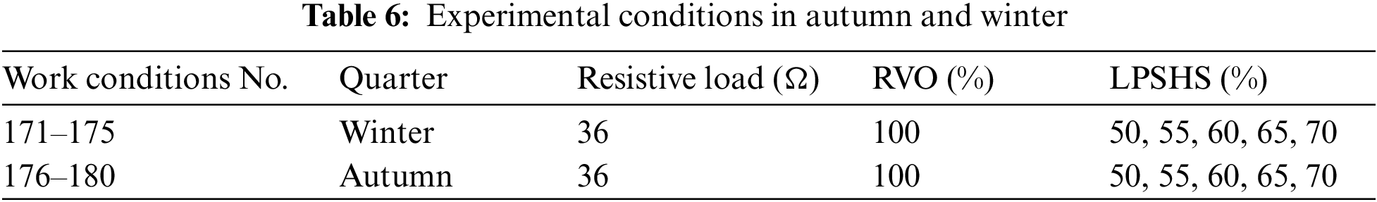
For working conditions No. 171–180, the ambient indoor temperature was 13°C in winter, and the central air conditioner was adjusted to simulate an ambient room temperature of 21°C in autumn. The system used R134a as the working medium, RVO was 100%, LPSHS was 50%–70%, and the resistive load of the generator was 36 Ω, as shown in Table 6.
4.1 Analyzing System Stability
According to the working conditions No. 1–20, as shown in Fig. 3. When the generator was not loaded, the inlet temperature and pressure of the expander stabilized at 39.80°C and 0.9 MPa, respectively, after 5 min of system operation. When the generator load was 36 Ω, the inlet temperature and pressure of the expander were approximately 39.60°C and 0.95 MPa, respectively.
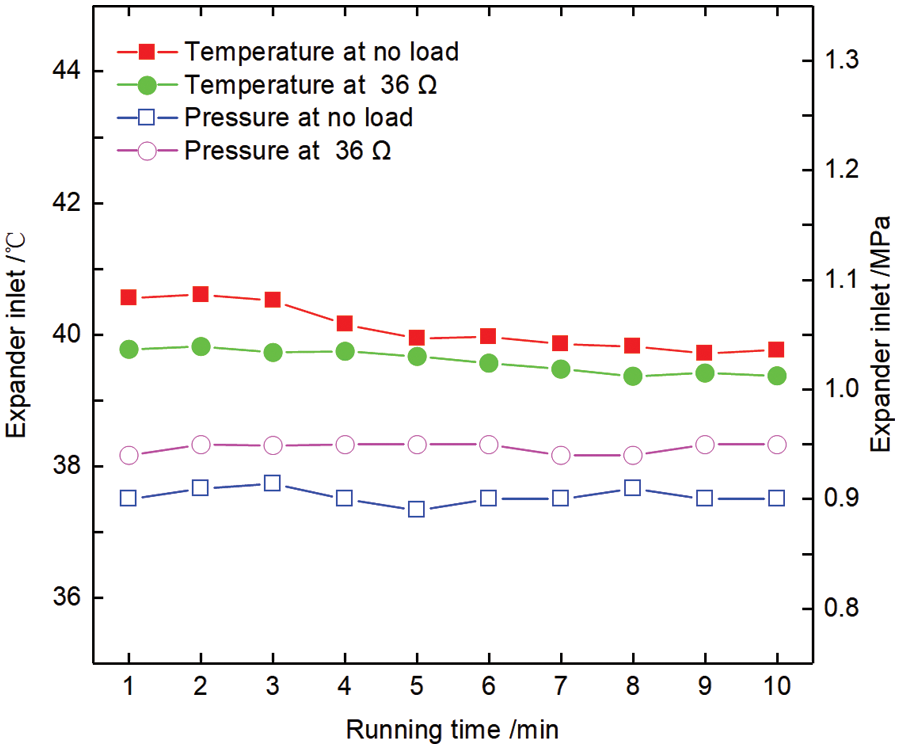
Figure 3: System stability
The results showed that the ORC system exhibits better stability when the generator has a resistive load.
4.2 Analyzing System Variations under Generator No-Load
Based on working conditions No. 21–45, as shown in Fig. 4, the SHST, MFR of the working medium, GS, and system generation voltage under different RVOs increase with the increase of LPSHS when the generator is unloaded.
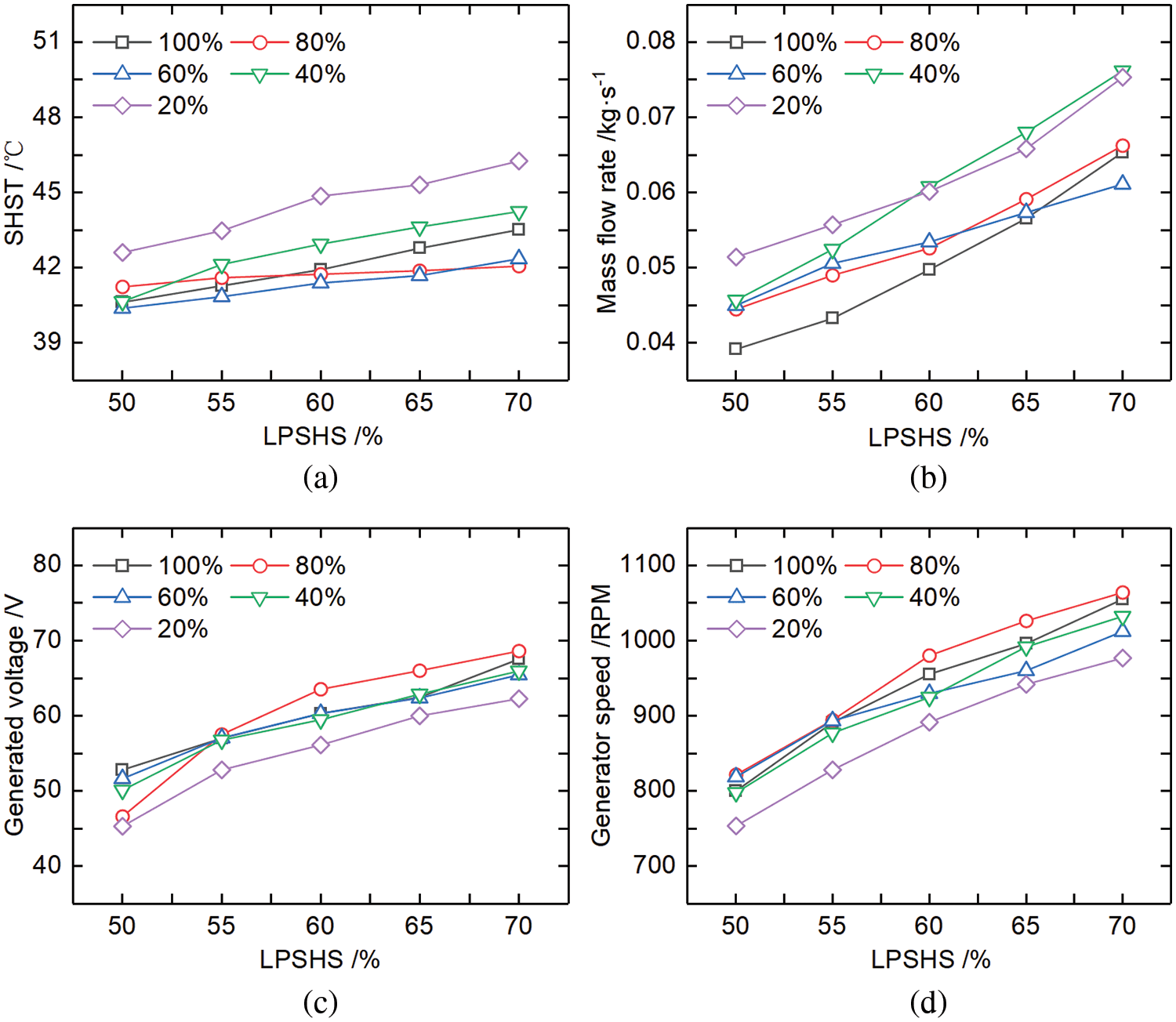
Figure 4: System variations with LPSHS and RVO without load (a) Simulated heat source temperature, (b) mass flow rate, (c) generated voltage, (d) generator speed
As shown in Fig. 4a, the SHST ranged from 40.38°C to 46.26°C. When RVO was 20% and LPSHS was 70%, the highest temperature was 46.26°C. As shown in Fig. 4b, the MFR of the working medium was set in a range of 0.039 kg/s to 0.076 kg/s. The slope of MFR was highest at 40 % of RVO. When the maximum MFR of the working medium was 0.076 kg/s, RVO was 40% and LPSHS was 70%. As shown in Fig. 4c, when the maximum generation voltage was 68.63 V, RVO was 80% and LPSHS was 70%. As shown in Fig. 4d, GS at an RVO of 20% was the lowest. When the maximum GS was 1064 RPM, the RVO was 80% and the LPSHS was 70%.
In a word, when the generator was unloaded, the SHST, MFR of the working medium, GS, and system generation voltage at different RVOs all increased with the increase of LPSHS. The SHST ranged from 40.38°C to 46.26°C. When the highest MFR of the working medium was 0.076 kg/s, RVO was 40% and LPSHS was 70%. When the maximum generation voltage was 68.63 V, RVO was 80% and LPSHS was 70%. When the maximum generator speed was 1064 RPM, RVO was 80 % and LPSHS was 70%.
4.3 Analyzing System Variations under Generator Load
4.3.1 Analyzing the Influence of SHST on the PG
From working conditions No. 46–170, as shown in Fig. 5, we can see that when the resistive load of the generator was constant, the system PG increased with the increase of SHST.
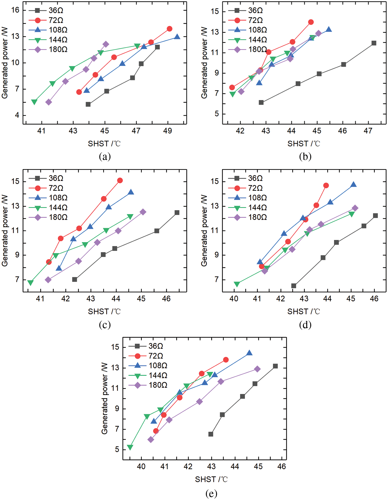
Figure 5: PG variations with different resistive loads and SHSTs (a) RVO 20%, (b) RVO 40%, (c) RVO 60%, (d) RVO 80%, (e) RVO 100%
When RVO was 20%, as shown in Fig. 5a, the PG of the system at 36 Ω load was the lowest with the increase of SHST. When the resistive load was 72 Ω and SHST was 49.11°C, the maximum power generation of the system was 13.91 W. As shown in Fig. 5b, when RVO was 40%, the PG of the system with 36 Ω load was the lowest among all the resistive loads with the increase of SHST. When the resistive load was 108, 144, and 180 Ω, the PG of the system was approximately equal, with the increase of the SHST. When the resistive load was 72 Ω and the SHST was 44.75°C, the maximum PG of the system was 14 W. From Fig. 5c, we can see that with the increase of SHST, the PG of the system at 36 Ω was the lowest load and at 72 Ω was the highest load when the RVO was 60 %. When the resistive load was 72 Ω and SHST was 44.15°C, the maximum PG of the system was 15.11 W. When RVO was 80 %, as shown in Fig. 5d, with the increase of SHST, the PG of the system with 36 Ω load was the lowest among all the resistive loads, and the slope of the system PG at a resistive load of 72 Ω was the highest load. When the resistive load was 108 Ω and SHST was 45.1°C, the maximum PG was 14.74 W. In Fig. 5e, one can find that with the increase of SHST, the PG of the system at 36 Ω was the lowest load, when the resistive load was 108 Ω and SHST was 44.61°C, the maximum PG of the system was 14.43 W.
Therefore, when RVO and the generator resistive load were constant, the PG of the system increased with the increase of SHST. When RVO was constant, with the increase of SHST, the PG of the system with 36 Ω load was the lowest among all the resistive loads. When RVO was 60%, the resistive load was 72 Ω and SHST was 44.15°C, the maximum PG of the system was 15.11 W.
4.3.2 Analyzing of SHST and MFR
Analyzing SHST Variation with Different RVO, Resistive Load, and LPSHS
For working conditions No. 46–170, as shown in Fig. 6, the SHST at different resistive loads increased with the increase of LPSHS when RVO kept the same.
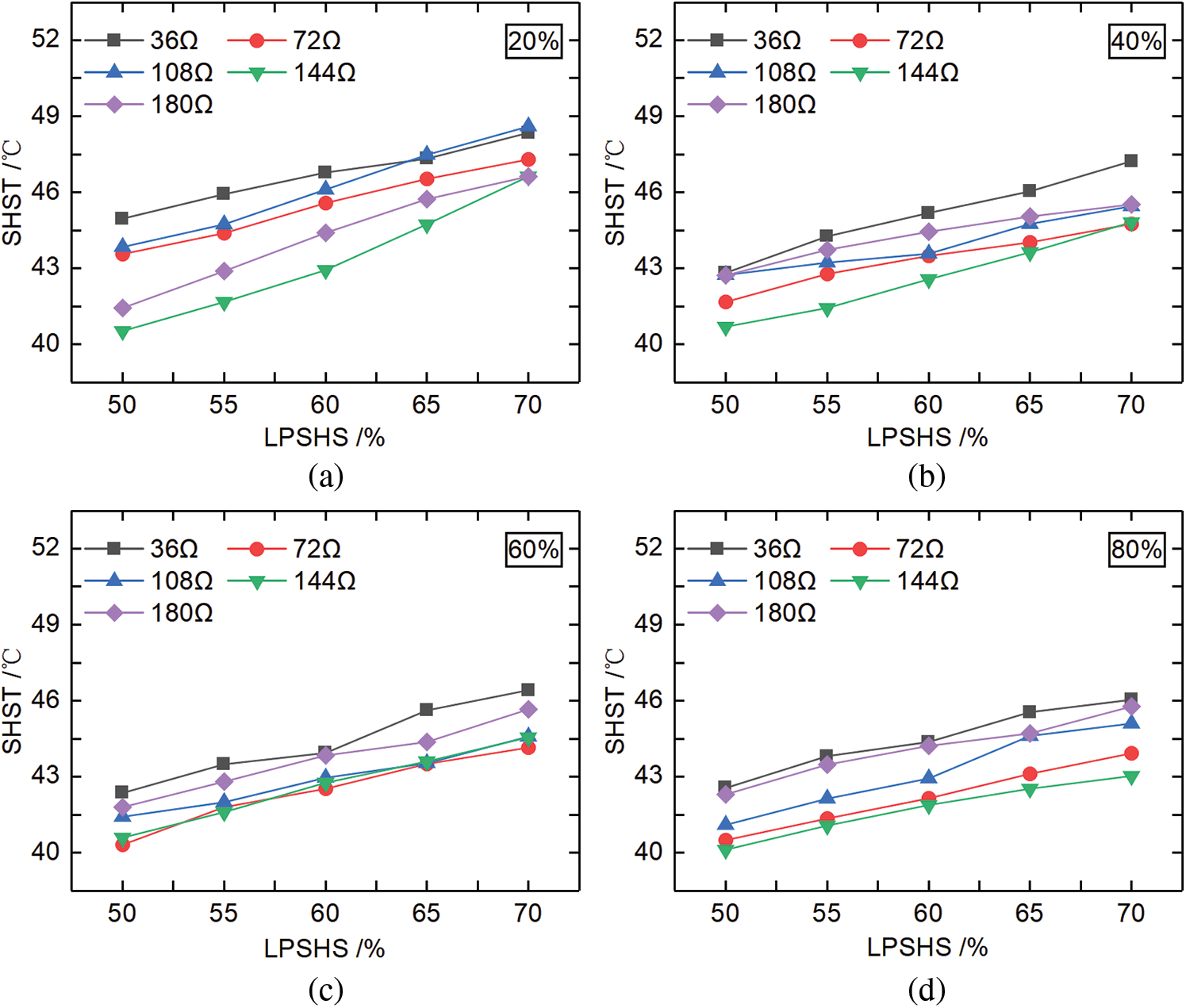
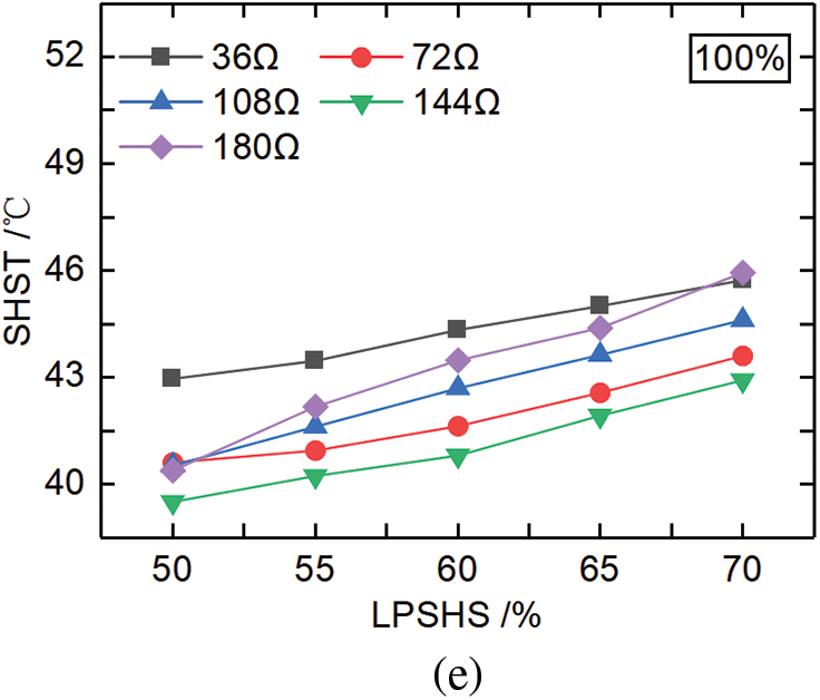
Figure 6: SHST variation with different RVOs, resistive loads, and LPSHSs (a) RVO 20 %, (b) RVO 40 %, (c) RVO 60%, (d) RVO 80%, (e) RVO 100%
As shown in Fig. 6a, when RVO was 20%, SHST varied from 40.53°C to 48.60°C, and the slope of the SHST was the highest at 144 Ω. As shown in Fig. 6b, when RVO was 40%, SHST changed from 40.70°C to 47.23°C, and the slope of SHST was the lowest at 108 Ω. When LPSHS was the same, the SHST was highest at 40% of RVO and 36 Ω of resistive load. As shown in Fig. 6c, when RVO was 60%, the SHST changed from 40.60°C to 46.42°C, and the slopes of SHST at different resistive loads were approximately equal. As shown in Fig. 6d, when RVO was 80%, the SHST varied from 40.12°C to 46.05°C, and the SHST was the highest at 36 Ω load and smallest at 144 Ω load. It can be seen from Fig. 6e that RVO was 100 %, the SHST changed from 39.51°C to 45.95°C, and the SHST was the lowest at 144 Ω of resistive load. The slopes of SHST were equal with 36, 108, and 144 Ω of loads.
The results showed that when RVO was the same, the SHST under different resistive loads increased with the increase of LPSHS, while the SHST varied from 39.51°C to 48.60°C. When SHST reached the maximum, the RVO was 20%, LPSHS was 70%, and the resistive load was 108 Ω.
Analyzing MFR Variation with Different RVOs, Resistive Loads, and LPSHSs
For working conditions No. 46–170, as shown in Fig. 7. When RVO was the same, the MFR of the working medium under different resistive loads increased with the increase of LPSHS.
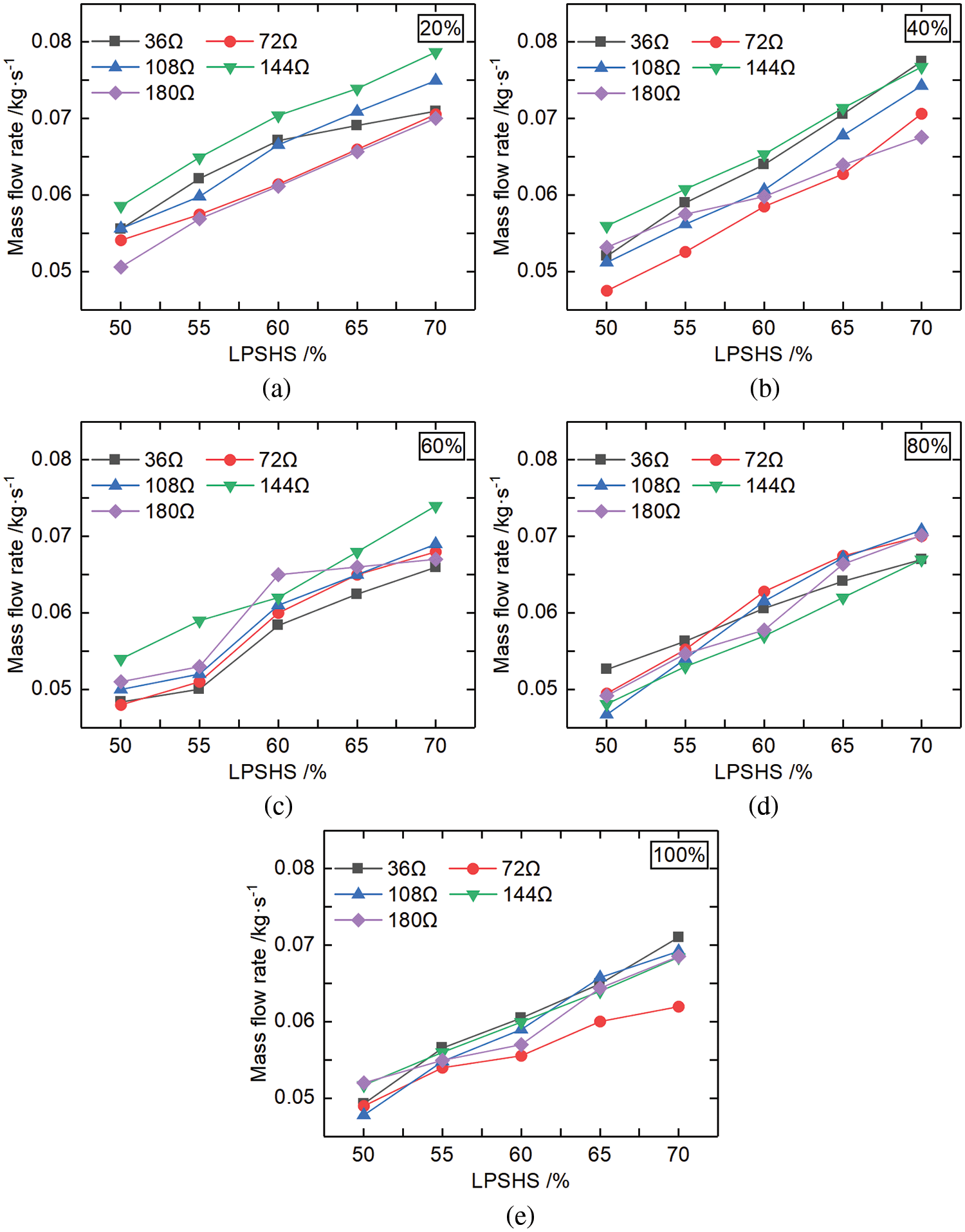
Figure 7: MFR variation for different RVOs, resistive loads, and LPSHSs (a) RVO 20%, (b) RVO40%, (c) RVO 60%, (d) RVO 80%, (e) RVO 100%
As shown in Fig. 7a, when RVO was 20%, the MFR of the working medium at 36 Ω load first increased and then decreased with the increase of LPSHS. When RVO was 20%, the MFR of the working medium at a resistive load of 144 Ω was the largest among all resistive loads. Moreover, the maximum MFR of the working medium was 0.079 kg/s at 70% of LPSHS and 144 Ω load. As shown in Fig. 7b, when RVO was 40%, the slope of the MFR of the working medium was the highest at 36 Ω load and lowest at 180 Ω load. The maximum MFR was 0.077 kg/s at 70% of LPSHS and 36 Ω load. In Fig. 7c, we can see that when the RVO was 60%, the MFR at 144 Ω load increased approximately linearly with the increases of LPSHS, and the maximum MFR was 0.074 kg/s at 70% of LPSHS and 144 Ω load. As shown in Fig. 7d, when RVO was 80%, the slope of the MFR was the lowest at 36 Ω load and highest at 108 Ω among all resistive loads. It can be seen from Fig. 7e that the maximum MFR was 0.071 kg/s at 70% LPSHS and 108 Ω load when RVO was 100%, and the slope of MFR was lowest at 72 Ω load.
The results indicated that, under the same RVO, the MFR of the working medium increased with the increase of LPSHS. For different RVOs and resistive loads, the MFR of the working medium was always maximum when LPSHS was 70%. When RVO was 20%, the maximum MFR of the working medium was 0.079 kg/s at 70% of LPSHS and 144 Ω load.
4.3.3 Analyzing EPR Variations with Different RVOs and LPSHSs
For working conditions No. 46–170, the resistive load of the generator was 36 Ω, as shown in Fig. 8. EPR fluctuated around 1.19 with 20% RVO. EPR was the lowest at 40% RVO, while LPSHS decreased EPR by about 60%. EPR has a linear relationship with 60% RVO. When RVO was 80%, the EPR fluctuated around 60% of LPSHS and then stabilized at 1.218. EPR fluctuated at 1.218 when RVO was 100%.
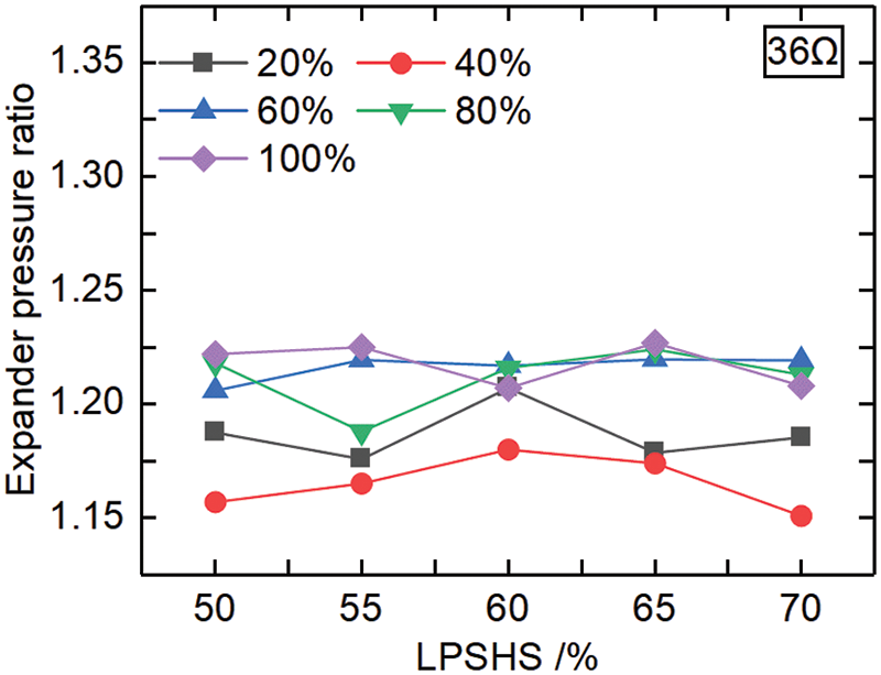
Figure 8: EPR variation with different RVO and LPSHS
The experiment showed that when the resistive load was the same, EPR fluctuated less, indicating better system stability.
Analyzing GS Variation with Different RVOs, Resistive Loads, and LPSHSs
For working conditions No. 46–170, as shown in Fig. 9. When RVO was the same, the GS increased with the increase of LPSHS under different resistive loads.
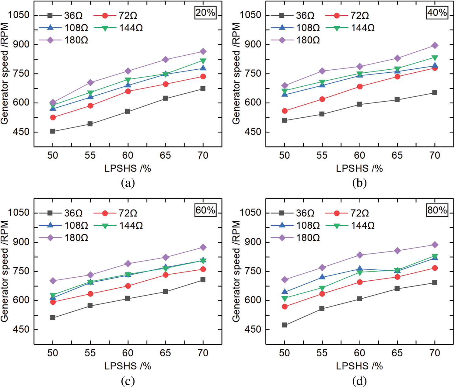
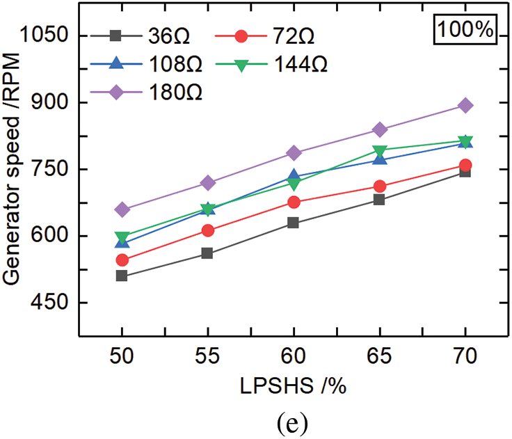
Figure 9: GS variations with different RVOs, resistive loads, and LPSHSs (a) RVO 20%, (b) RVO 40%, (c) RVO 60%, (d) RVO 80%, (e) RVO 100%
When the LPSHS was the same, GS increased with the increase of the resistive load. As shown in Fig. 9a, when LPSHS was 70%, the resistive load was 180 Ω, and RVO was 20%, the highest GS was 869 RPM. Fig. 9b showed when LPSHS was 70%, the resistive load was 180 Ω and RVO was 40%, the highest GS was 896 RPM. In Fig. 9c, we can see that the highest GS was 875 RPM, when LPSHS was 70%, the resistive load was 180 Ω and RVO was 60%. It can be seen from Fig. 9d that the highest GS was 888 RPM for LPSHS was 70%, the resistive load was 180 Ω and RVO was 80%. When LPSHS was 70%, the resistive load was 180 Ω and RVO was 100%, the highest GS was 894 RPM, as shown in Fig. 9e.
The experimental results showed that under the same RVO, GS increased with the increase of LPSHS, and the GS increased with the increase of resistive load when LPSHS was the same. Moreover, when LPSHS was 70%, the resistive load was 180 Ω and RVO was 40%, the highest GS was 896 RPM.
Analyzing PG Variation with Different RVOs, Resistive Loads, and LPSHSs
For working conditions No. 46–170, under the same RVO, the PG under different resistive loads increased with the increase of LPSHS can be found in Fig. 10.
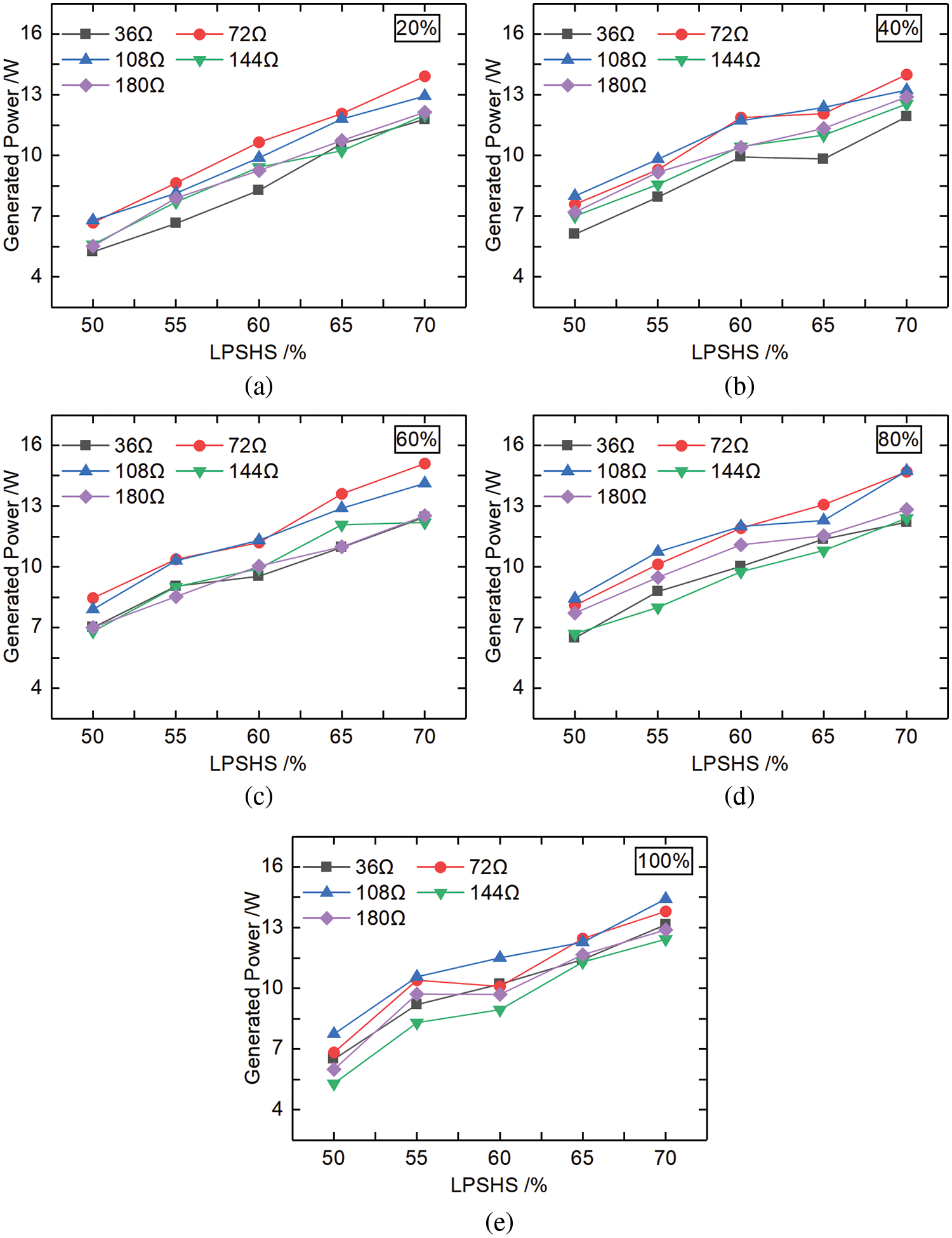
Figure 10: PG variation with different RVOs, resistive loads, and LPSHSs (a) RVO 20%, (b) RVO 40%, (c) RVO 60%, (d) RVO 80%, (e) RVO 100%
As shown in Fig. 10a, when RVO was 20%, LPSHS was 70% and the resistive load was 72 Ω, the highest PG was 13.91 W. Fig. 10b showed that when RVO was 40%, LPSHS was 70%, the resistive load was 72 Ω, the highest PG was 14 W. Under different resistive loads, PG increases initially and then slows down, about 60% of LPSHS. Among all resistive loads, the slope of PG is highest at 72 Ω and 60 % resistive load. We can see from Fig. 10c that when RVO was 60%, LPSHS was 70% and the resistive load was 72 Ω, the highest PG was 15.11 W. Besides, when RVO was 80%, LPSHS was 70%, and the resistive load was 108 Ω, the highest PG was 14.74 W, as shown in Fig. 10d. The slope of PG was linear at 72 Ω of resistive load. as shown in Fig. 10e when RVO was 100%, LPSHS was 70%, and the resistive load was 108 Ω, the highest PG was 14.43 W. The slope of the PG with 72, 144, and 180 Ω load was roughly equal. When the resistive load was 36 Ω and 108 Ω, PG rose faster and then slower around 55% of LPSHS.
The results indicated that when RVOs were the same, PG increased with the increase of LPSHS under different resistive loads. When RVO was 60%, LPSHS was 70%, the resistive load was 72 Ω, and the highest PG was 15.11 W.
In summary, when RVO and resistive load were constant, the PG of the system increased with the increase of SHST.
When RVO was the same, the SHST, MFR of the working medium, GS, and PG of the system increased with the increase of LPSHS under different resistive loads. The SHST changed from 39.51°C to 48.60°C. When SHST was maximum, RVO was 20%, LPSHS was 70%, and the resistive load was 108 Ω. The MFR of the working medium was always maximum when LPSHS was 70% for different RVOs and resistive loads. When RVO was 20%, LPSHS was 70% and the resistive load was 144 Ω, the highest MFR of the working medium was 0.079 kg/s. When the resistive load was the same, EPR fluctuated less, indicating better system stability.
The GS increased with the increase of resistive load when LPSHS and RVO were constant. The highest GS was 896 RPM when LPSHS was 70%, the resistive load was 180 Ω and RVO was 40%. When RVO was 60%, the SHST was 44.15°C, LPSHS was 70%, and the resistive load was 72 Ω, the highest PG was 15.11 W.
4.4 Analyzing of System Variation in Autumn and Winter
Fig. 11 shows the working conditions No. 171–180.
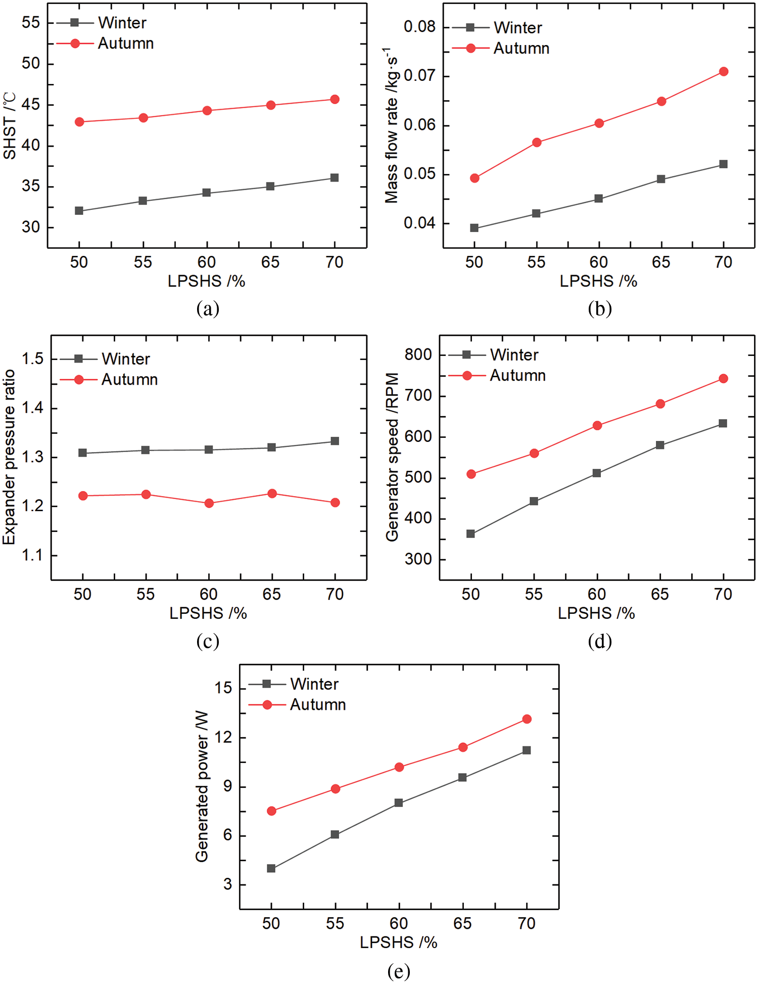
Figure 11: System variation in the autumn and winter (a) simulated heat source temperature, (b) mass flow rate, (c) expander pressure ratio, (d) generator speed, (e) generated power
From Fig. 11a, we can see that with the increase of LPSHS, the SHST in autumn was about 10°C higher than in winter. With the increase of LPSHS, the MFR of the working medium in autumn was about 0.02 kg/s higher than in winter, as shown in Fig. 11b. In Fig. 11c, it can be found that with the increase of LPSHS, EPR in winter was slightly higher than in autumn by 0.1. Fig. 11d illustrates that with the increase of LPSHS, the GS in autumn was about 119 RPM higher than in winter. It can be found in Fig. 11e that with the increase of LPSHS, PG in autumn was about 2.48 W higher than in winter.
The results indicated that with the increase of LPSHS, the SHST, MFR, GS, and PG of the system were higher in autumn than in winter, while the EPR was higher in autumn than in winter.
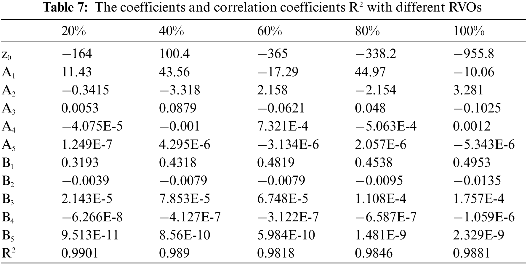
Based on the above experiments, the relationship equation between the LPSHS, resistive load, and PG was fitted, when RVO was 20% to 100%. As shown in Eq. (3):
where
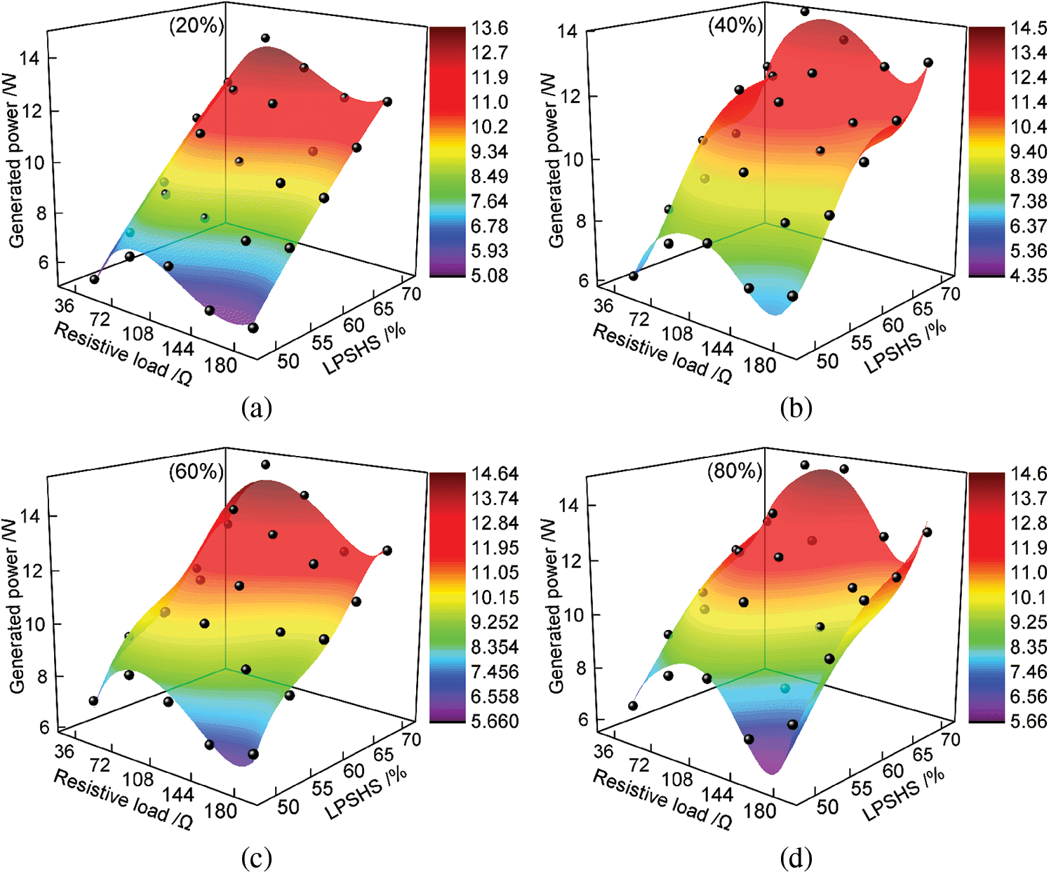
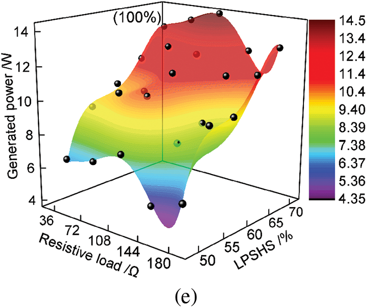
Figure 12: Fitted surfaces between LPSHS, resistive load, and PG with different RVOs (a) RVO 20%, (b) RVO 40%, (c) RVO 60%, (d) RVO 80%, (e) RVO 100%
Based on the original experimental equipment, adjustments were made to the RVO, resistive load, and LPSHS, and the PG was measured. Eq. (3) was verified when the RVO, resistive load and LPSHS were different. As shown in Fig. 13, the standard deviation between the calculated and experimental values of PG was within 0.0792, and the relative error was within ±5%. It was concluded that the fitted equation between LPSHS, resistive load, and PG was valid.
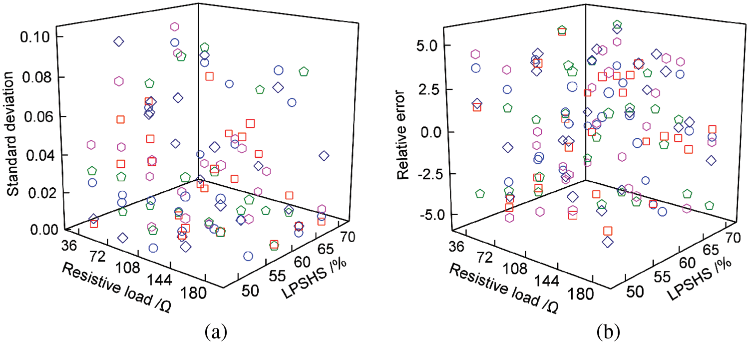
Figure 13: Experimental values and calculated values of PG when RVO varied from 20% to 100% (a) standard deviation, (b) relative error
In this paper, based on the ultra-low temperature heat source below 50°C, the performance of the ORC system was studied by adjusting the resistive load of the generator, the RVO, and the LPSHS. The following conclusions can be drawn:
● Compared to no resistive load, the stability of the ORC system is better when the generator has a resistive load.
● When the generator is unloaded, the SHST, MFR of the working medium, GS, and the voltage generated by the system with different RVO increase with the increase of LPSHS. The SHST varies from 40.38°C to 46.26°C. When RVO is 80% and LPSHS is 70%, the maximum generator voltage is 68.63 V, and the maximum GS is 1064 RPM.
● When the generator has a resistive load, the SHST, MFR of the working medium, GS, and PG of the system increase with the increase of the LPSHS for RVO remains the same. When RVO and the generator resistive load are constant, the PG increases with the increase of SHST. SHST changed from 39.51°C to 48.60°C. When SHST is at its maximum, the RVO is 20%, LPSHS is 70%, and the resistive load is 108 Ω. GS increases with the increase of resistive load when LPSHS and RVO are constant. The highest GS is 896 RPM when LPSHS is 70%, the resistive load is 180 Ω and RVO is 40%. When RVO is 60%, LPSHS is 70%, and the resistive load is 72 Ω, the highest PG of the system is 15.11 W.
● The SHST, MFR, GS, and PG are all higher in autumn than in winter. While EPR is higher in autumn than in winter.
● When RVO is the same, there is a correlation between LPSHS, resistive load, and PG, with a correlation coefficient of 0.9818 to 0.9901. The standard deviation between the calculated value and the experimental value of PG is within 0.0792, and the relative error is within ±5%. This relationship can provide strategic advice for power control output in the system.
● Based on a large number of experiments, the optimization direction of the ORC system under an ultra-low temperature heat source was obtained. In future redevelopment of ORC systems, it is necessary to reduce the rated power of the simulated heat source module and add a heat storage device inside it. It is also necessary to keep the diameter of the pipeline consistent in the system, and finally replace a new expander of the same type. This work has made some efforts in the research of ORC systems for ultra-low temperature heat sources.
Acknowledgement: None.
Funding Statement: This work was supported by Tianjin Natural Science Foundation (No. 21JCZDJC00750).
Author Contributions: The authors confirm contribution to the paper as follows: study conception and design: T. Zhou, X. Xu; data collection: T. Zhou, L. Zhang; results analysis and manuscript preparation: T. Zhou; grammar polishing: L. Hao, M. Si. All authors reviewed the results and approved the final version of the manuscript.
Availability of Data and Materials: All data generated or analysed during this study are included in this article.
Conflicts of Interest: The authors declare that they have no conflicts of interest to report regarding the present study.
References
1. Kılıç Depren, S., Kartal, M. T., Çoban Çelikdemir, N., Depren, Ö. (2022). Energy consumption and environmental degradation nexus: A systematic review and meta-analysis of fossil fuel and renewable energy consumption. Ecological Informatics, 70, 101747. https://doi.org/10.1016/j.ecoinf.2022.101747 [Google Scholar] [CrossRef]
2. Bu, S., Yang, X., Sun, Y., Li, W., Su, C. et al. (2022). Thermodynamic performances analyses and process optimization of a novel AA-CAES system coupled with solar auxiliary heat and organic Rankinecycle. Energy Reports, 8, 12799–12808. https://doi.org/10.1016/j.egyr.2022.09.133 [Google Scholar] [CrossRef]
3. Daniarta, S., Kolasinski, P., Imre, A. R. (2021). Thermodynamic efficiency of trilateral flash cycle, organic Rankine cycle and partially evaporated organic Rankine cycle. Energy Conversion and Management, 249, 114731. https://doi.org/10.1016/j.enconman.2021.114731 [Google Scholar] [CrossRef]
4. Özdemir Küçük, E., Kılıç, M. (2023). Exergoeconomic analysis and multi-objective optimization of ORC configurations via Taguchi-Grey Relational Methods. Heliyon, 9(4), e15007. https://doi.org/10.1016/j.heliyon.2023.e15007 [Google Scholar] [PubMed] [CrossRef]
5. Calli, O., Colpan, C. O., Gunerhan, H. (2021). Thermoeconomic analysis of a biomass and solar energy based organic Rankine cycle system under part load behavior. Sustainable Energy Technologies and Assessments, 46, 101207. https://doi.org/10.1016/j.seta.2021.101207 [Google Scholar] [CrossRef]
6. Köse, Ö., Koç, Y., Yağlı, H. (2022). Is Kalina cycle or organic Rankine cycle for industrial waste heat recovery applications? A detailed performance, economic and environment based comprehensive analysis. Process Safety and Environmental Protection, 163, 421–437. https://doi.org/10.1016/j.psep.2022.05.041 [Google Scholar] [CrossRef]
7. Hijriawan, M., Pambudi, N. A., Wijayanto, D. S., Biddinika, M. K., Saw, L. H. (2022). Experimental analysis of R134a working fluid on Organic Rankine Cycle (ORC) systems with scroll-expander. Engineering Science and Technology, An International Journal, 29, 101036. https://doi.org/10.1016/j.jestch.2021.06.016 [Google Scholar] [CrossRef]
8. Yang, J., Yu, B., Ye, Z., Shi, J., Chen, J. (2019). Experimental investigation of the impact of lubricant oil ratio on subcritical organic Rankine cycle for low-temperature waste heat recovery. Energy, 188, 116099. https://doi.org/10.1016/j.energy.2019.116099 [Google Scholar] [CrossRef]
9. Chen, H., Zhao, L., Cong, H., Li, X. (2022). Synthesis of waste heat recovery using solar organic Rankine cycle in the separation of benzene/toluene/p-xylene process. Energy, 255, 124443. https://doi.org/10.1016/j.energy.2022.124443 [Google Scholar] [CrossRef]
10. Shaofu, M., Bani Hani, E. H., Tao, H., Xu, Q. (2022). Exergy, economic, and optimization of a clean hydrogen production system using waste heat of a steel production factory. International Journal of Hydrogen Energy, 47(62), 26067–26081. https://doi.org/10.1016/j.ijhydene.2021.07.208 [Google Scholar] [CrossRef]
11. Loni, R., Mahian, O., Najafi, G., Sahin, A. Z., Rajaee, F. (2021). A critical review of power generation using geothermal-driven organic Rankine cycle. Thermal Science and Engineering Progress, 25, 101028. https://doi.org/10.1016/j.tsep.2021.101028 [Google Scholar] [CrossRef]
12. Sleiti, A. K., Al-Ammari, W. A., Al-Khawaja, M. (2023). Experimental investigations on the performance of a thermo-mechanical refrigeration system utilizing ultra-low temperature waste heat sources. Alexandria Engineering Journal, 71, 591–607. https://doi.org/10.1016/j.aej.2023.03.083 [Google Scholar] [CrossRef]
13. Pan, M., Chen, X., Li, X. (2022). Multi-objective analysis and optimization of cascade supercritical CO2 cycle and organic Rankine cycle systems for waste-to-energy power plant. Applied Thermal Engineering, 214, 118882. https://doi.org/10.1016/j.applthermaleng.2022.118882 [Google Scholar] [CrossRef]
14. Varis, C., Ozcira Ozkilic, S. (2023). In a biogas power plant from waste heat power generation syste-m using Organic Rankine Cycle and multi-criteria optimization. Case Studies in Thermal Engineering, 44, 102729. https://doi.org/10.1016/j.csite.2023.102729 [Google Scholar] [CrossRef]
15. Peng, H., Li, Y., Jia, X. (2022). Experimental study on thermoelectric generation Device based on accumulated temperature waste heat of coal gangue. Energy Reports, 8, 210–219. https://doi.org/10.1016/j.egyr.2022.05.095 [Google Scholar] [CrossRef]
16. Wang, H. X., Lei, B., Wu, Y. T. (2023). Simulations on organic Rankine cycle with quasi two-stage expander under cross-seasonal ambient conditions. Applied Thermal Engineering, 222, 119939. https://doi.org/10.1016/j.applthermaleng.2022.119939 [Google Scholar] [CrossRef]
17. Han, Y., Zhang, Y., Zuo, T., Chen, R., Xu, Y. (2020). Experimental study and energy loss analysis of an R245fa organic Rankine cycle prototype system with a radial piston expander. Applied Thermal Engineering, 169, 114939. https://doi.org/10.1016/j.applthermaleng.2020.114939 [Google Scholar] [CrossRef]
18. Wu, T., Meng, X., Wei, X., Han, J., Ma, X. (2020). Design and performance analysis of a radial inflow turbogenerator with the aerostatic bearings for organic Rankine cycle system. Energy Conversion and Management, 214, 112910. https://doi.org/10.1016/j.enconman.2020.112910 [Google Scholar] [CrossRef]
19. Wu, T., Wei, X., Meng, X., Ma, X., Han, J. (2020). Experimental study of operating load variation for organic Rankine cycle system based on radial inflow turbine. Applied Thermal Engineering, 166, 114641. https://doi.org/10.1016/j.applthermaleng.2019.114641 [Google Scholar] [CrossRef]
20. Yang, F., Zhang, H., Hou, X., Tian, Y., Xu, Y. (2019). Experimental study and artificial neural network based prediction of a free piston expander-linear generator for small scale organic Rankine cycle. Energy, 175, 630–644. https://doi.org/10.1016/j.energy.2019.03.099 [Google Scholar] [CrossRef]
21. Chen, W. H., Chiou, Y. B., Chein, R. Y., Uan, J. Y., Wang, X. D. (2022). Power generation of thermoe-lectric generator with plate fins for recovering low-temperature waste heat. Applied Energy, 306, 118012. https://doi.org/10.1016/j.apenergy.2021.118012 [Google Scholar] [CrossRef]
22. Zhou, J., Hai, T., Ali, M. A., Shamseldin, M. A., Almojil, S. F. (2023). Waste heat recovery of a wind turbine for poly-generation purpose: Feasibility analysis, environmental impact assessment, and parametric optimization. Energy, 263, 125891. https://doi.org/10.1016/j.energy.2022.125891 [Google Scholar] [CrossRef]
23. Shoeibi, S., Saemian, M., Khiadani, M., Kargarsharifabad, H., Ali Agha Mirjalily, S. (2023). Influence of PV/T waste heat on water productivity and electricity generation of solar stills using heat pipes and thermoelectric generator: An experimental study and environmental analysis. Energy Conversion and Management, 276, 116504. https://doi.org/10.1016/j.enconman.2022.116504 [Google Scholar] [CrossRef]
24. Kaczmarczyk, T. Z., Żywica, G. (2022). Experimental research of a micropower volumetric expander for domestic applications at constant electrical load. Sustainable Energy Technologies and Assessments, 49, 101755. https://doi.org/10.1016/j.seta.2021.101755 [Google Scholar] [CrossRef]
25. Cao, S., Xu, J., Miao, Z., Liu, X., Zhang, M. et al. (2019). Steady and transient operation of an organic Rankine cycle power system. Renewable Energy, 133, 284–294. https://doi.org/10.1016/j.renene.2018.10.044 [Google Scholar] [CrossRef]
26. Jin, Y. L., Gao, N. P., Zhu, T. (2022). Effect of resistive load characteristics on the performance of Organic Rankine cycle (ORC). Energy, 246, 123407. https://doi.org/10.1016/j.energy.2022.123407 [Google Scholar] [CrossRef]
27. Kaczmarczyk, T. Z., Żywica, G. (2022). Experimental study of a 1 kW high-speed ORC microturbogenerator under partial load. Energy Conversion and Management, 272, 116381. https://doi.org/10.1016/j.enconman.2022.116381 [Google Scholar] [CrossRef]
Cite This Article
 Copyright © 2024 The Author(s). Published by Tech Science Press.
This work is licensed under a Creative Commons Attribution 4.0 International License , which permits unrestricted use, distribution, and reproduction in any medium, provided the original work is properly cited.
 Downloads
 Citation Tools