Peak Shaving Strategy of Concentrating Solar Power Generation Based on Multi-Time-Scale and Considering Demand Response

Nomenclature

1  Introduction

With the continuous access of new energy sources such as wind power, the safety and economy of power system operations are facing new challenges. Due to its strong intermittency and uncertainty, wind power exhibits strong anti-peak shaving characteristics after being connected to the power system, which causes certain difficulties in dispatching and operating the power system [1]. In order to cope with the impact of wind power’s reverse peak regulation characteristics on the operation of the power system and to better utilize and absorb wind power, corresponding peak regulation strategies need to be formulated. At present, peak shaving tasks in the power system are mainly undertaken by conventional thermal power units and hydropower units. However, when thermal power units participate in peak shaving, the operating economy of the units will be affected. Especially when deep peak shaving is performed, not only the economy but also the operation security and stability of the units are threatened. Although the hydropower unit has a good peak shaving capacity, due to its storage capacity and the limitation of the incoming water volume, it only participates in the system peak shaving in dry seasons and uses the full-load power generation method to avoid water abandonment in wet seasons, which means it has certain seasonal restrictions.

In recent years, another form of new energy power generation—solar thermal power generation—has been rapidly developed. Equipped with a large-capacity heat storage system, it can achieve 24-h continuous power generation, thus making this type of solar power generation overcome the phenomenon of traditional photovoltaic power generation stopping at day and night, but with more stability [2]. In addition, the CSP generator set can quickly adjust its own output up to 20% per minute at the fastest, far higher than that of ordinary thermal power generators, to provide certain climbing support for the system’s peak shaving. It takes a very short time from the stop state to the full power state during the operation process, so it can also be quickly started and stopped peaking [3]. Therefore, CSPs participating in power system peak shaving can well alleviate the pressure of system peak shaving and realize the replacement of one new energy source with another.

With the development of smart grids, the operation and dispatch of the power system have gradually changed from the traditional single generation-side resource dispatching to joint generation-side resource dispatching, where DR is also developed on this basis. By calling demand-side resources, users can interact with power companies in two directions, so that traditional rigid loads have a certain degree of flexibility, which is conducive to the safe and economic operation of the power grid.

Shi et al. [4] studied the dispatch model of CSP plant grid-connected operation and analyze the benefits of CSP plant grid-connected operation. Ying et al. [5] studied the multi-day self-dispatch model of CSP plants in power systems and analyze different predicted time scales for dispatch results. Du et al. [6] established a day-ahead dispatch and operation simulation model with consideration of demand-side response under large-scale wind power grid connections. Usaola et al. [7] studied the effect of electricity price-based demand response resources on unit commitment and wind power grid integration. Chen et al. [8] proposed an optimal dispatch method that takes into account the uncertainty of wind power and demand response and adopts the phase-robust mixed integer programming method to solve the model. Li et al. [9] established a SCUC model based on stochastic programming and respond to wind power on the demand side.

However, the above-mentioned literature mostly focuses on the day-ahead scheduling model for each generation-side resource and demand response resource without giving further consideration to its multi-timescale. For power generation resources, the start-up and shutdown costs of the unit account for a large proportion of the total unit operating cost. Therefore, reasonable arrangements for the unit’s start-up and shutdown are the primary prerequisites for the economic operation of the unit. The minimum start-stop time of the unit ranges from a few hours to tens of hours and is related to the operating conditions of other units, the load level over a longer period, and other factors. Therefore, the plan for starting and stopping peak shaving units should be formulated on a larger time scale to ensure the rationality of the start-stop program. When arranging the output of the generating units, considering that the forecast errors of wind power decrease with the shortening of the time scale, it is necessary to optimize the arrangement of unit output on a relatively shorter time scale as much as possible. In addition, due to the wide variety of demand response resources involved in system peak shaving and their response capabilities, some (such as temperature-controllable loads) can respond to dispatch signals immediately, while others (such as motors) need to be arranged before the scheduled date. Generally speaking, the accuracy of wind power forecasting tends to increase significantly with the shortening of the forecast time scale. Therefore, the peak shaving optimization model is in line with the principle of “looking ahead into the future and back into the past” to rationalize the start and stop, output, and demand response resources of each unit. If all of them are incorporated into the day-ahead scheduling model for unified optimization, it will be difficult to give full play to the adjustment capabilities of various scheduling resources at different time scales.

Jin et al. [10] and Wang et al. [11], according to the idea of hierarchical refinement, proposed a multi-time-scale scheduling model based on four-time scales of “day ahead, day within 1 h, day within 15 min, and real-time” to provide a useful reference for optimally scheduling power systems based on multiple time scales. However, the dispatch model established in reference [12] only considered the adjustments of the power of each unit and the demand-side response and does not discuss the total cost of system operation, the combination of each unit, or the output. Although reference [13] considered the above factors, the scheduling model established is still based on the day-ahead scheduling model architecture, making it relatively simple to consider the in-day and real-time parts.

Based on the comprehensive consideration of the multi-time-scale characteristics of power generation and demand-side resources, this paper establishes a multi-time-scale peak shaving optimization model with three levels of “week”, “day ahead” and “in-day”, which not only optimizes the demand response resources at different time scales by layers, but also formulates the start-stop and output scheme of each unite at different scales on the basis of considering the operation characteristics of power generation resources such as solar thermal units and conventional units. In the day-ahead peak shaving optimization model, based on the characteristics of the fast start and stop of CSP units, SSP is put forward to deal with the influence of wind power forecast uncertainty on the optimization results. Finally, the validity of the model is verified by a calculation example.

2  The Basic Architecture of a Multi-Time-Scale Peak Shaving Optimization Model

With the gradually increasing proportion of wind power connected to the grid, new requirements are put forward for the peak shaving of the power system. On the one hand, due to the strong correlation between wind power prediction accuracy and time scale, in order to overcome the impact of wind power uncertainty in power system dispatch, all kinds of resources should be optimized in a short time as much as possible. On the other hand, the various resources involved in system peak shaving have multi-time-scale characteristics, and a single day-ahead scheduling model is bound to make it difficult to coordinate the various scheduling resources. Therefore, it is necessary to establish a peak shaving optimization model that carefully considers various resources and multiple time scales and reasonably schedules various scheduling resources.

Based on the above considerations, this paper establishes a CSP peak-shaving optimization model based on multiple time scales and taking into account the demand-side response. The model mainly includes the following schedulable resources:

(1)   Resources on the power generation side According to the difference between the minimum start-stop times, the units are divided into conventional units and CSP ones. Conventional units take a long time to start and stop. The start and stop plans of the units need to be determined in the weekly peak shaving plan to ensure their rationality, while the CSP units can start and stop quickly within a very short time, so the start and stop plans can be Confirmed in the peak shaving plan a few days ago.

(2)   Demand-side resources. Demand-side resources can be roughly divided into two types: price-based PDR and IDR. When demand-side resources participate in system peak shaving, PDR needs to be determined in the day-ahead peak shaving optimization mode. IDR can be scheduled in real-time in the in-day peak shaving optimization model.

In order to reasonably schedule resources with different time-scale characteristics, this paper proposes a rolling peak shaving optimization model containing three levels of week, day ahead, and in-day with multi-time-scale characteristics in reference [14]. Therefore, corresponding scheduling schemes can be determined at different levels and on different time scales. Among them, the optimization result determined in the upper-level scheduling model can be used as the input of the following model; that is, it can be regarded as a known quantity in the following model:

(1)   Weekly peak shaving plan: execute once a week (with a resolution of 2 h). The task of week-peak regulation is to determine the unit composition of conventional units.

(2)   Day-ahead rolling peak shaving plan: execute every 1 h (with a resolution of 1 h). The task of day-ahead peak shaving is to determine the unit combination of CSP units and the day-ahead PDR response strategy.

(3)   In-day rolling peak shaving plan within the day: execute once every 15 min (with a resolution of 15 min). The task of peak shaving within the day is to determine the output of all units and the IDR response strategy.

3  Establishment of a Multi-Time-Scale Peak Shaving Optimization Model

After determining the peak shaving optimization model structure, three different time scales are supposed to be modeled and solved separately. In view of the uncertainties in the forecasting process of wind power, the traditional day-ahead dispatch model can no longer adapt to the peak shaving and dispatching requirements of modern power systems, so targeted modeling methods are needed. At present, for the randomness of wind power forecasting, the modeling method based on stochastic programming is mainly adopted. Stochastic programming can be divided into several branches, which can be generally classified into the following two types: CCP [15,16] and SSP [17–20]. The core idea of the CCP method is to set a certain confidence level for the constraint condition, and the probability of the constraint condition being established is not less than the confidence level. This method actually relaxes the constraint condition to a certain extent so that the search can be carried out over a wider range. The core idea of the SSP method is to use a certain method (such as Monte Carlo sampling) to generate a variety of possible scenarios based on the distribution law of uncertain resources (such as wind energy, solar energy, etc.), and then compare the similarities among these scenarios. The scenes are reduced, and a number of representative scenes left are fitted in the scheduling model for optimization and solution, so that the decision variables can be adapted to any of the scenes. As a result, the group with the lowest expected cost is taken to be the optimal solution. In this paper, given the impact of the uncertainty of wind power forecasting on peak shaving, SSP is adopted in day-ahead scheduling to improve the robustness of the start-stop strategy and PDR response strategy of CSP units.

3.1 Weekly Peak Shaving Optimization Model

3.1.1 Objective Function

The main purpose of the weekly peak shaving plan is to determine the unit composition of the conventional units. Therefore, a weekly peak shaving optimization model takes the minimum total system operating cost as the objective function, as in Eqs. (1) and (2).

minOC(1)

OC=∑iN∑t=1T(C(Pi,t)+ui,tGi,t)+∑t=1T(λtlossDtloss)+∑t=1T(λtWcurtWtcurt)(2)

where N is the number of conventional units; T is the duration of the dispatching cycle; Pi,t and C(Pi,t) are the power generation and cost of the conventional unit at time t, respectively; Gi,t is the start-up and shutdown cost of the conventional unit; ui,t is the start-stop state variables of unit i at time t, where 1 indicates that the unit is in the start-up state, and 0 indicates that the unit is in shutdown state; Dtloss, Wtcurt are the load shedding power and abandonment power of the system at t, respectively; λtloss, λtWcurt are the load shedding penalty cost of the system at t and wind curtailment costs,which is 500–CNY/MWh.

3.1.2 Constraints

(1) Active power balance constraint as in Eq. (3).

∑i=1NPi,t+(Wt−Wtcurt)+∑j=1MPi,tCSP=Dt−Dtloss(3)

where Wt is the predicted value of wind power at time t; M is the number of CSP units in the system; Pi,tCSP is the power generation of the CSP generator set at time t; Dt is the predicted value of system load at time t; Dtloss is the value of system load shedding at time t.

(2) The upper and lower limits of the active power of conventional generators as in Eq. (4).

ui,tPimin≤Pi,t≤ui,tPimax(4)

where Pimin, Pimax are the upper and lower limits of the active power output of the conventional unit.

(3) Climbing constraints of a conventional generator as in Eq. (5).

−RDi≤Pi,t−Pi,t−1≤RUi(5)

where RUi, −RDi are the up and down ramp rate limits of conventional generator sets, respectively.

(4) The upper and lower limits of the active power of the CSP generator as in Eq. (6).

PjCSP,min≤Pj,tCSP≤PjCSP,max(6)

where PjCSP,min and PjCSP,max are the upper and lower limits of the active output of the j-th CSP unit.

(5) Start and stop constraints of the conventional generator as in Eq. (7).

{(ui,t−1−ui,t)+(ui,t+τ−ui,t+τ−1)≤1,∀τ∈[1,⋯,Di−1](ui,t−ui,t−1)+(ui,t+τ−1−ui,t+τ)≤1,∀τ∈[1,⋯,Oi−1](7)

where Di, Oi are the minimum shutdown and start-up time of the unit, respectively.

3.1.3 Optimized Results

In this paper, the widely used commercial optimization software CPLEX is employed for modeling and solving so as to determine the unit composition of conventional units within a week. The result will be directly substituted into the day-ahead and in-day peak shaving models as a known quantity to solve other unknowns.

3.2 Day-Ahead Rolling Peak Shaving Optimization Model

3.2.1 Objective Function

In the day-ahead peak shaving optimization model, electricity price needs to be considered, making maximum total social welfare the objective function for optimization as in Eq. (8).

maxGS−OC(8)

where GS is consumer surplus and OC is total production cost as in Eq. (9), both of which can be expressed as in Eq. (10).

GS=∑t=1TρtPDRt(9)

OC=∑i=1N∑t=1T∑s=1NSπsC(Pi,s,t)+∑t=1T∑s=1NS(πsλs,tlossDs,tloss)+∑t=1T∑s=1NS(πsλs,tWcurtWs,tWcurt)(10)

where ρt is the electricity price at time t; PDRt is the PDR response power at time t; NS is the number of wind power prediction scenarios; πs is the probability of occurrence of the s-th scenario; Pi,s,t is the generation power of the conventional unit at time t under scenario s; λs,tloss and λs,tWcurt are the load shedding penalty cost and wind abandonment cost of the system at time t in the s scenario, respectively; and Ds,tloss, Ws,tWcurt respectively are the load shedding power and abandon wind power of the system at time t and in the s scenario.

3.2.2 Main Constraints

(1) Active power balance constraint as in Eq. (11).

∑i=1NPi,s,t+∑j=1MPj,s,tCSP+(Ws,t−Ws,tWcurt)=Ds,t+PDRt−Ds,tloss(11)

where Pj,s,tCSP is the generating power of the CSP generator set at time t under scene s; Ds,t is the original load at time t under scene s; Ds,tloss is the value of system load shedding at time t under scene s.

(2) Constraints on the active output of CSP generators as in Eq. (12).

xj,tPj,tCSP,min≤Pj,s,tCSP≤xj,tPj,tCSP,max(12)

where xj,t is the start-stop state variable of the CSP unit at time t, for which 1 indicates the start-up and running state of the unit, while 0 means shutdown, respectively; Pj,tCSP,max and Pj,tCSP,min are the upper and lower limits active output of the CSP unit at time t.

(3) Climbing constraints of CSP generator units as in Eq. (13).

−RDjCSP≤Pj,s,tCSP−Pj,s,t−1CSP≤RUjCSP(13)

where RUjCSP and −RDjCSP are the up and down climbing rate limits of the CSP generator set, respectively.

(4) Start-stop restriction of CSP generator as in Eq. (14).

{(xj,t−1−xj,t)+(xj,t+τ−xj,t+τ−1)≤1,∀τ∈[1,⋯,DjCSP−1](xj,t−xj,t−1)+(xj,t+τ−1−xj,t+τ)≤1,∀τ∈[1,⋯,OjCSP−1](14)

where DjCSP, OjCSP are the minimum shut-down and start-up time of the unit, respectively.

(5) Constraints on the flexible adjustment capability of the unit as in Eq. (15).

{|Pi,s,t−Pi,bs,t|≤Δi|Pj,s,tCSP−Pj,bs,tCSP|≤ΔjCSP(15)

where Pi,bs,t, Pj,bs,tCSP are the optimized output results of conventional units and CSP units in the baseline scenario, respectively. Δi and ΔjCSP are the flexible adjustment capabilities of the two types of units. This constraint can ensure the conversion of the unit’s active output between any two scenarios without exceeding the limit.

(6) PDR response constraints

Also, since electricity price demand-side resource PDR was added to the day-a-day peak shaving optimization model, such resources should be limited to make sure that scheduling is done in a sensible way, as shown in Eqs. (16)–(18).

PDRtmin≤PDRt≤PDRtmax(16)

∑t=1TPDRt=0(17)

ρt≥Ce¯(18)

where PDRtmin and PDRtmax are the upper and lower limits of the PDR’s response capacity at the time t, representing the unit power cost. Among them, Eq. (16) can ensure that the net load adjustment amount of the demand side resources participating in the system peak shaving in one day is zero, that is, only the user’s power consumption time is adjusted, the user load is not reduced.

3.2.3 Optimization Results

After modeling and solving the day-ahead rolling peak shaving optimization model with CPLEX, the following optimization results for the decision variable can be obtained:

(1)   CSP generator unit combination;

(2)   Day-ahead PDR response strategy.

These values will be input into the lower in-day rolling peak shaving optimization model together with the results obtained in the upper weekly peak shaving optimization model as known quantities to solve other unknowns.

3.3 In-Day Rolling Peak Shaving Optimization Model

3.3.1 Objective Function

In the in-day peak shaving optimization model, it is necessary to determine the output of each unit and the IDR response strategy, so the minimum system operating cost is the objective function as in Eqs. (19) and (20).

minOC(19)

OC=∑t=1TC(Pi,t)+∑t=1TλIDRIDRt+∑t=1T(λtlossDtloss)+∑t=1T(λtWcurtDtWcurt)(20)

where λIDR is the incentive demand response compensation price; IDRt is the system incentive load response power at time t.

3.3.2 Main Constraints

(1) Active power balance constraint as in Eq. (21).

∑i=1NPi,t+∑j=1MPj,tCSP+(Wt−Wtcurt)=Dt+PDRt+IDRt−Dtloss(21)

where IDRt is the incentive load response at time t.

(2) Constraints on the active output of each unit as in Eq. (22).

{ui,tPimin≤Pi,t≤ui,tPimaxxj,tPjCSP,min≤Pj,tCSP≤xj,tPjCSP,max(22)

where the value ui,t and xj,t are determined in the weekly peak shaving and day-ahead peak shaving plan, which is the fixed value.

(3) Climbing constraints of each unit as in Eq. (23).

{−RDi≤Pi,t−Pi,t−1≤RUi−RDjCSP≤Pj,tCSP−Pj,t−1CSP≤RUjCSP(23)

(4) IDR constraint as in Eq. (24).

IDRmin≤IDRt≤IDRmax(24)

where IDRmax and IDRmin represent the maximum and minimum values of the incentive load response at time t, respectively.

3.3.3 Optimization Results

Through modeling and solving the in-day peak shaving optimization model using CPLEX, the following optimization results of decision variables can be determined:

(1)   Output of the CSP;

(2)   Output of conventional units;

(3)   IDR response strategy.

4  Example Analysis

4.1 Overview of the Model

Based on the actual power supply ratio structure of the actual power system in a certain area in the northwest, Fig. 1 is the schematic diagram of the actual power system structure. This paper simulates the addition of CSP stations to design calculation examples, thus further simulating and verifying the proposed dispatching model. The model consists of four conventional power-generating units, three CSP-generating units, and a wind farm. The PDR response capacity in the system is 10% of the total load, while the IDR response capacity is not more than 5% of the total load. The model is solved by the currently advanced commercial optimization software, CPLEX, in which the specific parameters of each unit are shown in Tables 1 and 2. The PDR price is shown in Table 3.

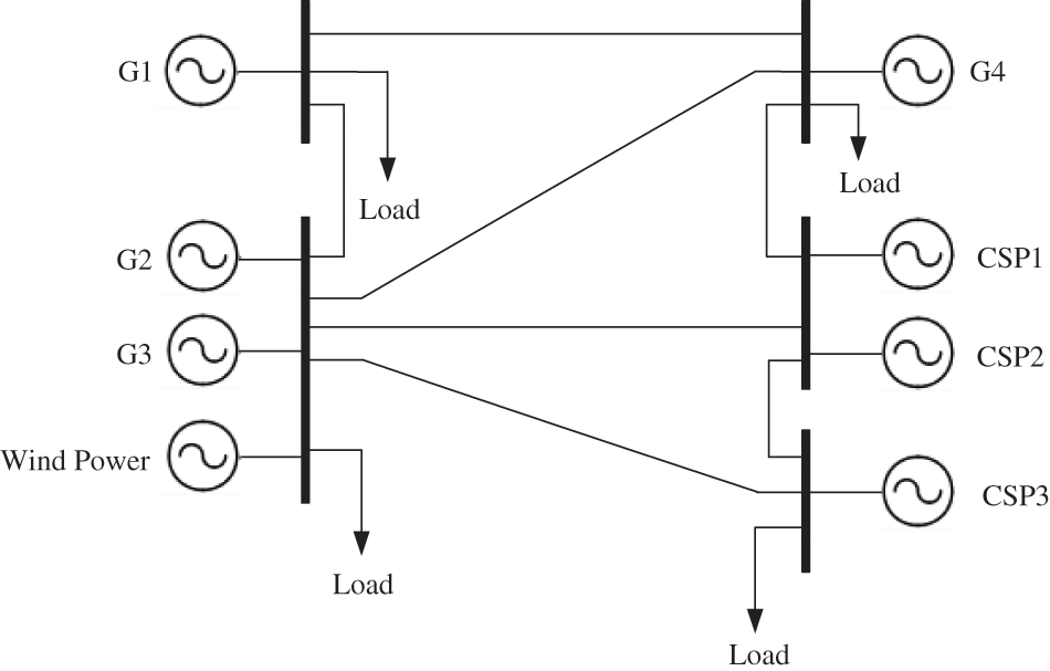
Figure 1: Schematic diagram of actual power system structure

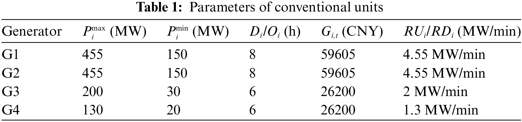
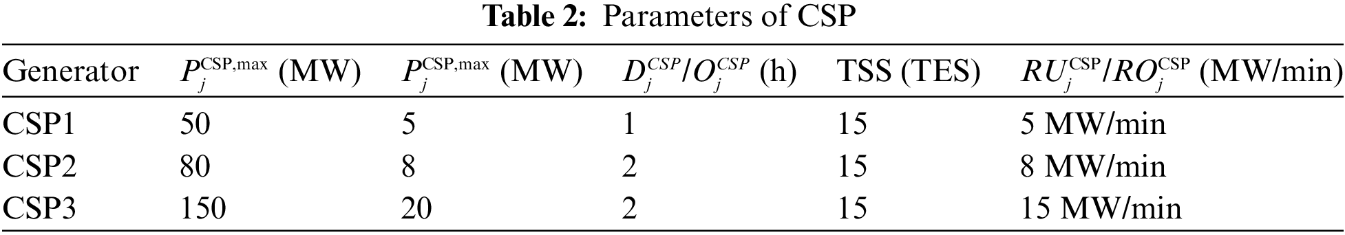
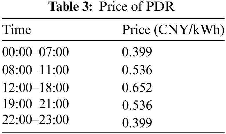
Fig. 2 shows the forecast curves of load and wind power at different time scales, and Fig. 3 shows the predicted values of direct normal irradiance (DNI) within a week. Assuming that the weekly prediction error of wind power is 35%, then the weekly prediction curve of wind power can be obtained by adding white noise with an expectation of 0 and a standard deviation of 0.35 to the actual wind power curve. Similarly, assuming that the forecast errors of wind power forecast before and during the day are 20% and 5%, and the forecast errors of the load during the week, day ahead, and in-day are 5%, 3%, and 1%, respectively, then the corresponding forecast curve can be obtained by adding the corresponding white noise on the basis of the actual curve. In addition, five working days (heavy-load days) and two rest days (small-load days) are considered in the weekly load, and two consecutive cloudy days (Thursday and Friday) are considered in the in-week DNI forecast. The subsequent calculation examples are all carried out on the basis of the above prediction curve.

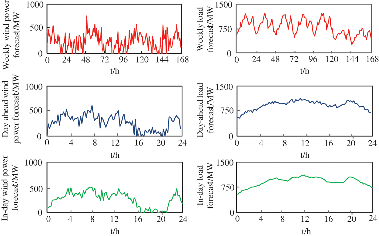
Figure 2: Wind power and load prediction curves under different time scales

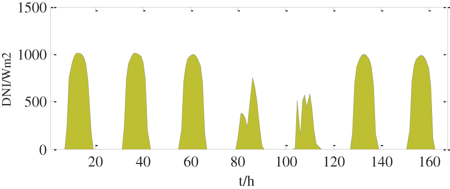
Figure 3: DNI prediction in one week

4.2 Analysis of the Results of Resource Scheduling

In order to study the utilization of all scheduling resources, the calculation examples were used to solve the weekly, day-ahead, and in-day peak shaving plans. First, the weekly peak shaving plan is calculated, and then the day-ahead and in-day peak shaving plans are respectively solved in a rolling way. Finally, continuous week-day-day rolling peak-shaving optimization results can be obtained by connecting the optimization results of each period. In the example, the day-ahead scheduling model uses the SSP-based stochastic planning model, with the number of scenarios being 5.

4.2.1 Analysis of Weekly Peak-Shaving Results

By solving the weekly peak shaving optimization model, the combination of conventional units within a week can be obtained, as shown in Fig. 4. It can be seen that for conventional thermal power units, in order to ensure the economic performance of the system and the stability of unit operation, the small unit (unit 4 in the figure) should be started first when the load level is low. As the load continues to rise, other units will be started gradually (such as unit 3 in the figure), and only when the load has risen to a certain level, that is, when the small unit can no longer meet the load demand, will the large units get started (e.g., units 1 and 2 in the figure). Once the large-scale units are turned on, they will mainly bear the base load and waist load of the system for a period of time in the future, so as to minimize the number of starts and stops and avoid the high operating cost caused by frequent starts and stops. It can also be seen from the figure that the number of start and stop times of the two large units in a week is significantly less than that of the other two small units.

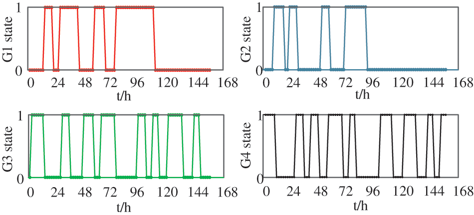
Figure 4: Conventional units commitment in one week

4.2.2 Result Analysis of Day-Ahead Peak Shaving Scheduling

Using the results of the conventional unit combination in the weekly peak shaving plan as the input data of the day-ahead peak-shaving model, and combined with SSP (a total of 5 wind power scenarios are considered), the day-ahead peak shaving optimization model can be solved to further determine the CSP unit combination PDR response strategy. Fig. 5 shows the day-ahead unit combination of conventional units (in this example, Monday is taken as an example), and Fig. 6 shows the five wind power scenarios selected in this article.

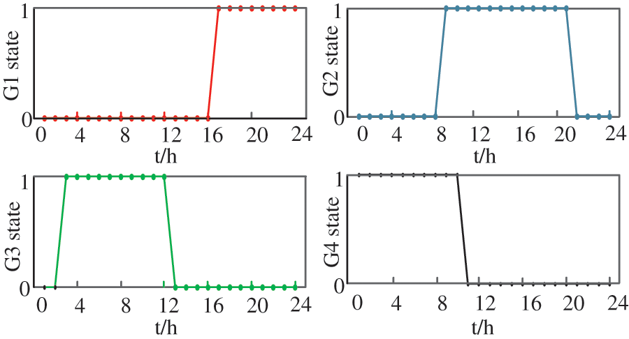
Figure 5: Conventional units commitment in day ahead

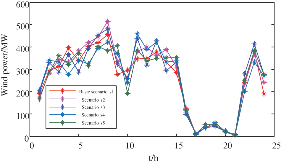
Figure 6: Wind power scenarios

By solving the day-ahead peak shaving optimization model, the day-ahead PDR response strategy and CSP combination can be obtained, as shown in Figs. 7 and 8. It can be seen from Fig. 7 that by optimizing the electricity price for each time period, the PDR can be guided to appropriately transfer the load according to different electricity prices, that is, to arrange the load power consumption and increase the load level during the low electricity price period (load low period: 01:00–08:00, 14:00–18:00, 22:00–24:00) as much as possible. In the peak electricity price period (peak load period: 08:00–14:00, 18:00–22:00), the load is reduced by the same amount to decrease the load demand during this period, which is equivalent to shifting the peak period load to the trough period while ensuring the user’s overall power consumption remains unchanged, thereby effectively reducing the peak-valley difference of the system. Fig. 8 shows the start-stop plan of CSP units determined a few days ago, from which we can see that in order to ensure the economy of system operation, CSP units carry out frequent start-stop peak shaving within a day, greatly reducing the load pressure for conventional thermal power units. At the same time, in order to ensure the power generation of large CSP units (such as CSP3), the frequency of start-stops is significantly less than that of small units.

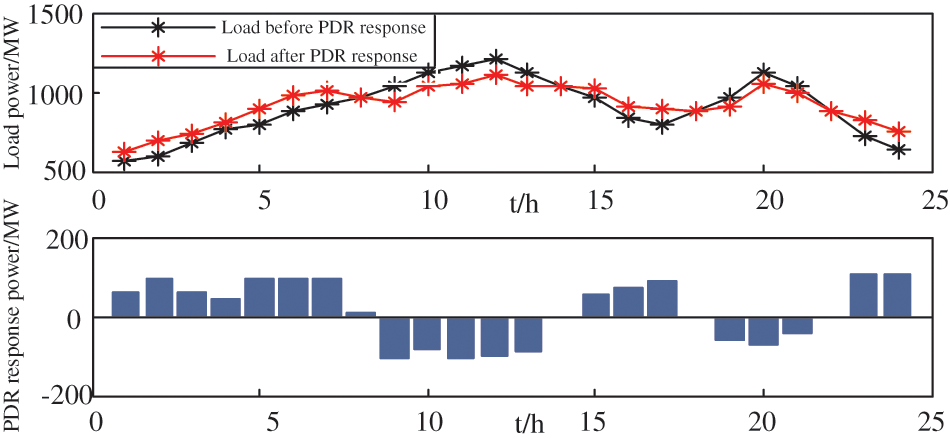
Figure 7: The response strategy of PDR

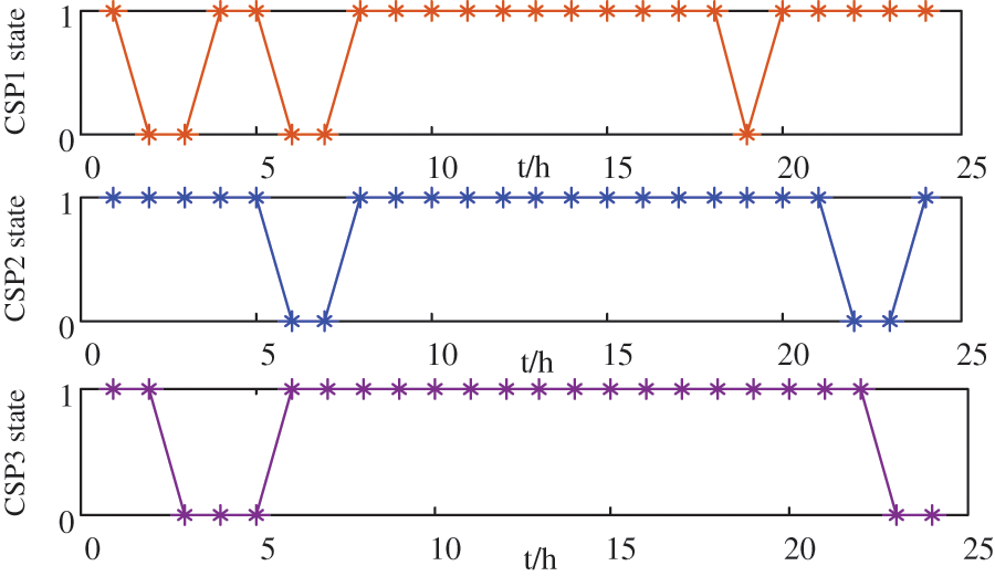
Figure 8: The unit commitment of CSP

4.3 Analysis of the Results of In-Day Peak Shaving Scheduling

As can be seen from Figs. 9 and 10, in the daytime, due to the high system load level and the relatively sufficient peak shaving capacity of the system, the wind power volatility has little impact on the system. At this time, to ensure the solar thermal power generation capacity, the three solar thermal units are all at full capacity, and conventional units are responsible for daily peak shaving tasks. At night, due to the low load level, some conventional units are in a shutdown state, and the night is a period with heavy winds and strong volatility, resulting in a serious shortage of adjustable capacity. At this time, CSP uses the energy stored in the heat storage system during the day for peak shaving, frequently adjusts its own output to cope with wind power, and provides a certain peak shaving capacity for the system. In addition, it can be seen from Fig. 11 that during system operation, IDR can be regarded as a system spinning reserve. When wind power changes drastically, IDR provides a certain peaking capacity for the system by adjusting its own load power, thereby undertaking part of the drastic changes in wind power.

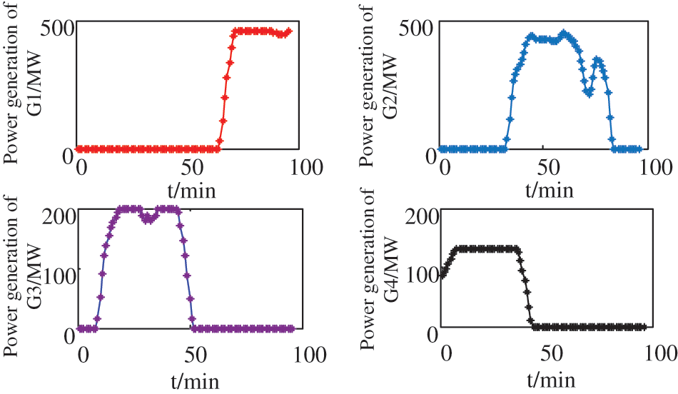
Figure 9: The power generation of conventional units

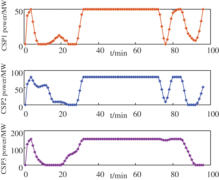
Figure 10: The power generation of CSP

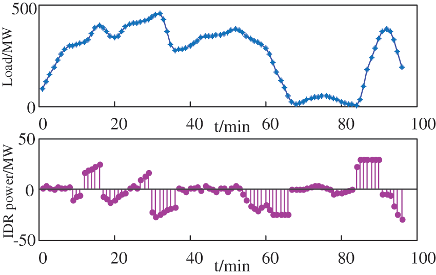
Figure 11: The response strategy of IDR

In the in-day rolling peak shaving, the conventional and CSP unit combination and PDR response are used as the inputs, and the scheduling period is 2 h with a resolution of 15 min. The optimization is carried out point by point, and the IDR response is considered to determine the output and IDR of each unit. The response strategy is shown in Figs. 11–13.

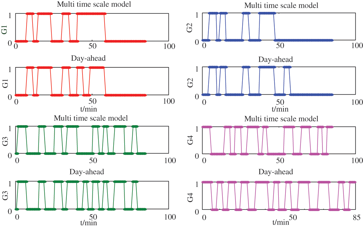
Figure 12: Comparison of conventional units commitment

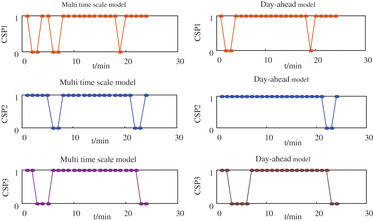
Figure 13: Comparison of CSP units commitment

4.4 Comparison with Traditional Scheduling Methods

In order to conduct a comparative study, traditional day-ahead scheduling methods are also considered in the following calculation examples. To ensure fairness in comparison, the proportions of PDR and IDR in the day-ahead scheduling model are the same as those mentioned in this paper. Wind power and load forecast power follow the previous forecast curve in this article. In the scheduling process, only the day-ahead scheduling model is used to coordinate and optimize various resources within 24 h, which means that not only the conventional unit combination and the CSP unit combination but also the output of each unit and the PDR and IDR responses are determined the day before.

As shown in Fig. 12, the conventional unit startup and shutdown schemes obtained under two different models are shown. It can be seen from the figure that under the traditional day-ahead scheduling model, G1 and G2 units start and stop 10 times, G3 units start and stop 18 times, and G4 units start and stop 20 times. Under the model proposed in this article, the number of starts and stops for G1 and G2 units is reduced to 8, and the number of starts and stops for G3 and G4 units is reduced to 16.

Therefore, compared with the traditional day-ahead scheduling model, the multi-time scale rolling optimization model proposed in this paper effectively reduces the number of starts and stops of conventional units, among which G1, G2, and G3 units are reduced twice, and G4 units are reduced four times. Reduce startup and shutdown costs by approximately 124,100 CNY.

As shown in Fig. 13, the startup and shutdown schemes of the CSP unit are obtained under two different models. It can be seen from the figure that under the traditional day-ahead scheduling model, the number of CSP1 starts and stops is 4, the number of CSP2 starts and stops is 2, and the number of CSP3 starts and stops is 3.

In the model proposed in this article, CSP1 has 6 start-stop times, CSP2 has 4 start-stop times, and CSP3 has 3 start-stop times.

Compared with the traditional day-ahead scheduling model, under the multi-time scale rolling optimization model proposed in this paper, the solar thermal units give full play to the characteristics of CSP rapid startup and shutdown to provide peak shaving support for the system, and their startup and shutdown times are significantly higher than the traditional model, which effectively alleviates the peak shaving pressure of the system and reduces the startup and shutdown times of conventional units.

Figs. 14 and 15 show the system’s PDR and IDR responses in the two modes. From the figure, it can be seen that the system PDR responses in the two modes are basically the same, while the IDR response is quite different: The IDR called for by the traditional day-ahead scheduling model in the peak shaving process is much higher than the model proposed in this article. As the IDR response of the model mentioned in this article is determined during the in-day dispatch phase and the accuracy of in-day wind power and load forecasting is higher than the previous forecast, only a small amount of the higher-cost IDR can meet the system’s peak shaving requirements. However, in the traditional day-ahead scheduling model, all schedulable resources are determined in the day-ahead scheduling stage, and the accuracy of day-ahead wind power and load forecasting is low. Therefore, in order to ensure the required system reserve capacity, a large number of IDRs with higher costs are needed as spare capacity to compensate for the uncertainty of wind power, which also increases the cost of system peak shaving.

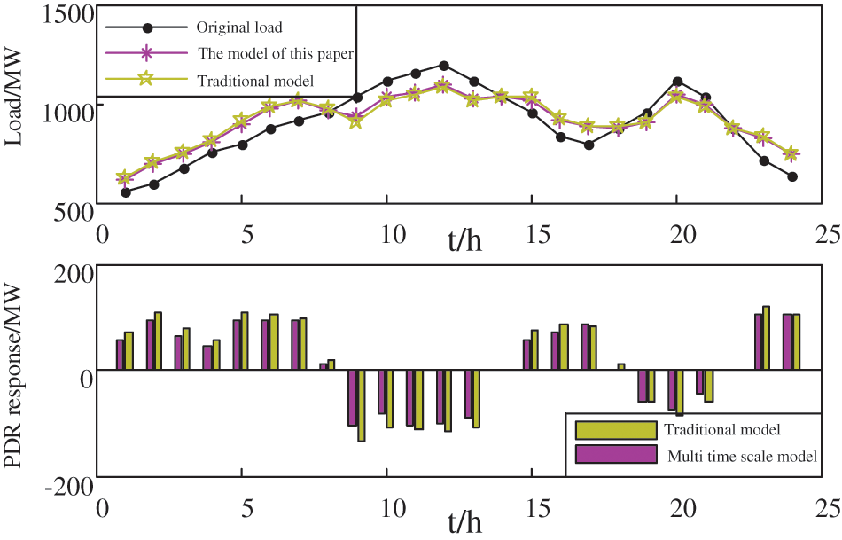
Figure 14: PDR response strategy under two modes

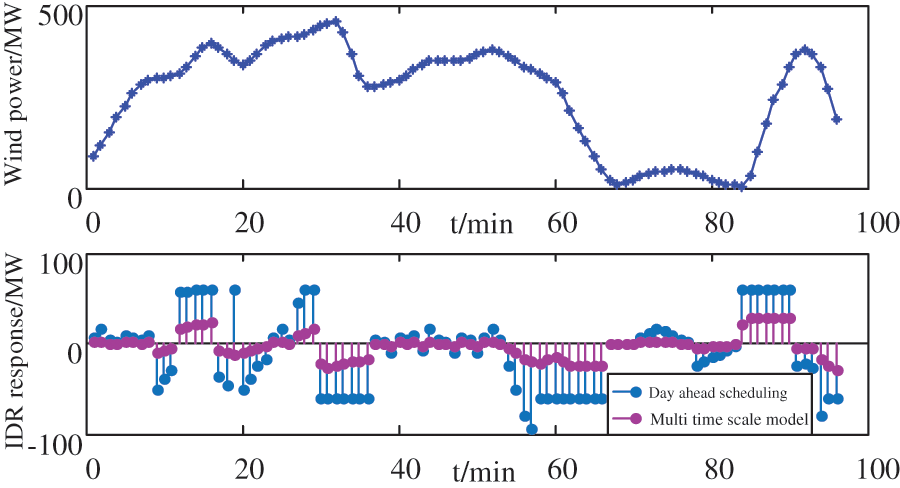
Figure 15: IDR response strategy under two modes

4.5 Peak-Shaving Utility Analysis

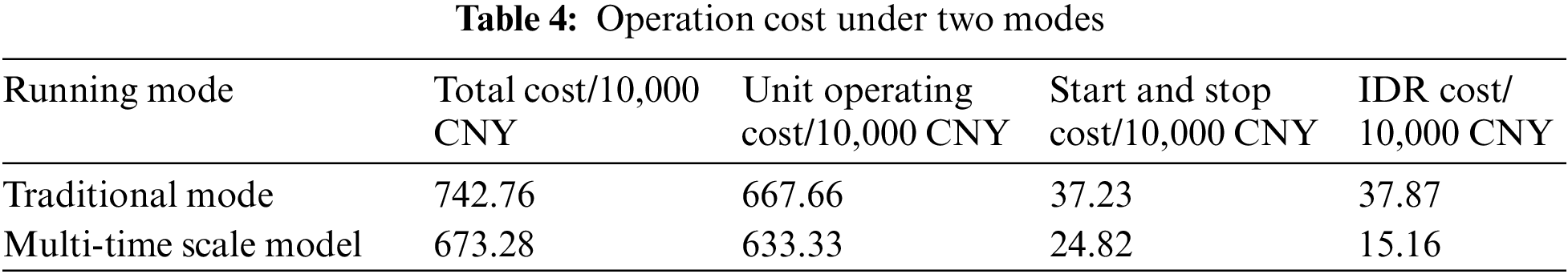
By comparing the results of the two scheduling modes, it can be found that when the traditional day-ahead peak shaving model is used, the total spinning reserve required by the system is about 85.98 MW. When the multi-time-scale rolling peak shaving model proposed in this paper is used, the total spinning reserve required by the system is about 8.69 MW, which only accounts for 10.1% of the peak shaving model. Moreover, the operating costs of the system under the two models are shown in Table 4.

5  Conclusion

This paper proposes a CSP peak-shaving strategy based on multiple time scales and taking into account the demand-side response. The model fully considers the multi-time-scale characteristics of conventional units, CSP units, and various demand-side resources. The CSP rolling peak shaving optimization model of a three-time scales-week, day-ahead, and in-day—realizes the interaction between peak shaving between the power generation side and the demand side. The calculation results show that:

The peak shaving optimization model based on multiple time scales can make full use of the characteristics of the power generation and demand-side resources in the system on different time scales for peak shaving. Among them, for the unit composition and output arrangements of conventional units and CSP units, the model optimizes them on different time scales, which not only effectively reduces the start-up and shutdown costs of conventional units in operation but also makes full use of CSP units’ feature of rapid start-stop to improve the flexibility of CSP units participating in power system peak shaving. In addition, the model also optimizes it separately in the day-ahead and in-day stages according to the different response speeds on the demand side, so that not only the PDR with a slower response speed participates in the peak and valley filling of the system, but also the IDR with a faster response speed is employed as part of the system’s spinning reserve to smooth out short-term fluctuations in wind power.

The rolling peak shaving model can, according to the characteristics of wind power and load forecasting accuracy be gradually improved as the time scale shrinks, effectively utilizing the wind power and load forecast results at each time scale, thereby improving the accuracy of the dispatch results. Compared with the day-ahead scheduling model, the rolling model proposed in this paper requires less spinning reserve capacity, which can effectively reduce the system operating cost and the impact of wind power uncertainty on system operation. In addition, this article also combines SSP, so as to improve the reliability of system operation.

It can be seen from the calculation results that when the traditional peak shaving model is used, the total operating cost of the system reaches about 7,427,600 CNY, but when the multi-time scale model is used, the total operating cost of the system is only 6,732,800 CNY, saving about 9.4% of the total cost. Among them, the start-stop cost in this mode is about 248,200 CNY, which is 33.3% lower than the traditional mode. And the IDR call cost is about 151,600 CNY, 59.9% lower than the traditional mode.

At the same time, the research in this paper still has shortcomings; for example, the economic benefits of the CSP plant are not considered in the model in this paper. Therefore, in the follow-up research process, the department will carry out a special study on this.

Acknowledgement: None.

Funding Statement: The authors thankfully acknowledge the support of the projects Youth Science Foundation of Gansu Province (Source-Grid-Load Multi-Time Interval Optimization Scheduling Method Considering Wind-PV-CSP Combined DC Transmission, No. 22JR11RA148) and Youth Science Foundation of Lanzhou Jiaotong University (Research on Coordinated Dispatching Control Strategy of High Proportion New Energy Transmission Power System with CSP Power Generation, No. 2020011).

Author Contributions: The authors confirm their contribution to the paper as follows: study conception and design: Lei Fang, Dong Haiying; data collection: Li Shuaibing, Lei Fang; analysis and interpretation of results: Lei Fang, Dong Haiying, Zhen Xiaofei; draft manuscript preparation: Lei Fang. All authors reviewed the results and approved the final version of the manuscript.

Availability of Data and Materials: The data comes from the simulation data for Western China. Most of the data has been presented in the form of graphs in the text, so no data list is given.

Conflicts of Interest: The authors declare that they have no conflicts of interest to report regarding the present study.

References

1. Chen, C. Q., Li, X. R., Zhang, B. Y. (2022). Energy storage peak and frequency modulation cooperative control strategy based on multi-time-scale. Power System Protection and Control, 50(5), 94–105. [Google Scholar]

2. Niu, J. Y., Wang, D. L., Yu, X., Guo, L. J., Sun, C. et al. (2022). Parameter optimization of low inertia power system to improve wind power consumption level. Electric Machines and Control, 26(2), 111–120. [Google Scholar]

3. Wei, W., Jiang, F., Dai, S. F. (2022). Economic optimization of deep peak regulation of thermal power units taking into account the risk of emergency storage on the demand side. Power System Protection and Control, 50(10), 153–162. [Google Scholar]

4. Shi, Q. S., Ding, J. Y., Liu, K. (2019). Economic optimal operation of microgrid integrated energy system with electricity, gas and heat storage. Electric Power Automation Equipment, 39(8), 269–276+293. [Google Scholar]

5. Ying, Y. Q., Wang, Z. F., Wu, X. (2020). Multi-objective strategy for deep peak shaving of power grid considering uncertainty of new energy. Power System Protection and Control, 48(6), 34–42. [Google Scholar]

6. Du, E. S., Zhang, N., Kang, C. Q. (2016). Reviews and prospects of the operation and planning optimization for grid integrated concentrating solar power. Proceedings of the CSEE, 36(21), 5765–5775 (In Chinese). [Google Scholar]

7. Usaola, J. (2013). Operation of concentrating solar power plants with storage in spot electricity markets. IET Renewable Power Generation, 81, 38–42. [Google Scholar]

8. Chen, R. Z., Sun, H. B., Li, Z. S. (2014). Grid dispatch model and interconnection benefit analysis of concentrating solar power plants with thermal storage. Automation of Electric Power Systems, 38(19), 1–6. [Google Scholar]

9. Li, J. L., Guo, Z. D., Ma, S. L. (2022). Overview of the “source-grid-load-storage” architecture and evaluation system under the new power system. High Voltage Engineering, 1, 1–14. [Google Scholar]

10. Jin, H. Y., Sun, H. B., Guo, Q. L. (2016). Multi-day self-scheduling method for combined system of CSP plants and wind power with large-scale thermal energy storage contained. Automation of Electric Power Systems, 40(11), 17–22. [Google Scholar]

11. Wang, B. B., Liu, X. C., Li, Y. (2013). Day-ahead generation scheduling and operation simulation considering demand response in large-capacity wind power integrated systems. Proceedings of the CSEE, 33(22), 35–44 (In Chinese). [Google Scholar]

12. De, J. C., Hobbs, B. F., Belmans, R. (2014). Value of price responsive load for wind integration in unit commitment. IEEE Transactions on Power Systems, 29(2), 675–685. [Google Scholar]

13. Zhao, C. Y., Wang, J. H., Watson, J. P. (2013). Multi-stage robust unit commitment considering wind and demand response uncertainties. IEEE Transactions on Power Systems, 28(3), 2708–2717. [Google Scholar]

14. Liu, X. C., Wang, B. B., Li, Y. (2014). Unit commitment model and economic dispatch model based on real time pricing for large-scale wind power accommodation. Power System Technology, 38(11), 2955–2963. [Google Scholar]

15. Yang, S. C., Liu, J. T., Yao, J. G. (2014). Model and strategy for multi-time scale coordinated flexible load interactive scheduling. Proceedings of the CSEE, 34(22), 3664–3673 (In Chinese). [Google Scholar]

16. Yao, J. G., Yang, S. C., Wang, K. (2014). Framework and strategy design of demand response scheduling for balancing wind power fluctuation. Automation of Electric Power Systems, 38(9), 85–92. [Google Scholar]

17. Yang, S. B., Tan, Z. F., Lin, H. Y., Li, P., De, G. et al. (2020). A two-stage optimization model for park integrated energy system operation and benefit allocation considering the effect of time-of-use energy price. Energy, 195(15), 117013. [Google Scholar]

18. Long, J., Mo, Q. F., Zeng, J. (2011). A stochastic programming based short-term optimization scheduling strategy considering energy conservation for power system containing wind farms. Power System Technology, 35(9), 133–138. [Google Scholar]

19. Ela, E., O’Malley, M. (2012). Studying the variability and uncertainty impacts of variable generation at multiple time-scales. IEEE Transactions on Power Systems, 37(3), 1324–1333. [Google Scholar]

20. Liu, M. H., Tian, S., Liang, Y. D. (2022). Double-level multi-objective optimal scheduling of microgrid considering customer satisfaction of electric vehicles. Distributed Energy, 7(2), 18–25. [Google Scholar]