Design of a Multifrequency Signal Parameter Estimation Method for the Distribution Network Based on HIpST

1  Introduction

PMU estimates the amplitude and phase of voltage and current waveform signals in the power grid, providing the power grid with time-stamped phasor and frequency information [1,2]. A traditional PMU focuses on the fundamental frequency and cannot completely cover the 0–2.5 kHz signal [3]. The large-scale access of distributed sources and load injects harmonics of different components into the distribution networks, increasing the difficulty of protection and fault detection of the distribution network [4]. Harmonic phasors have become a topic of significant interest in the distribution grid’s PMUs, as they can provide additional information for applications such as protection and fault diagnosis in the distribution grid [5–7]. Therefore, The synchronization measurement method needs to consider multifrequency estimation, fast response, and practicability.

Most existing practical and low-complexity synchronization measurement methods are based on discrete Fourier transform (DFT) and Taylor series and achieve synchronous measurement estimation via different improvements in these series. Indeed, because it is easy to understand and simple to calculate, DFT has been widely used in PMU [8–12]. DFT-based algorithms include enhanced interpolated DFT (E-IpDFT) [8], the DFT improvement method [9,10], iterative interpolated DFT(I-IpDFT) [11], and others [13]. Especially in the distribution network, due to the intermittence and volatility of the source network load, the DFT-based quantity measurement method is limited in solving negative spectral line interference and dynamic signal parameter estimation. Therefore, based on interpolated DFT (IpDFT), Paolo et al. [8] further proposed the E-IpDFT algorithm, eliminating the negative spectral line error and improving the estimation accuracy through two IpDFT calculations. Based on IpDFT, Asja et al. [11] proposed the I-IpDFT, which improves the accuracy of dynamic signal parameter estimation through multiple iterative calculations. Based on IpDFT and Hilbert Transform, Guglielmo et al. [12] proposed the method effectively to solve the problems of spectrum leakage and noise interference. However, the calculation amount has increased under the condition of large frequency deviation and signal dynamic change, and the application of iterative calculations in the embedded platform has been limited.

To improve the accuracy of parameter estimation under dynamic signal changes, the Taylor series and its improved algorithm are further proposed in references [14–19]. The algorithms based on the Taylor series are Taylor Extended Kalman Filtering [14,15], adaptive algorithm [15], Maximally Fla Differentiators [17], Taylor weighted least squares (TWLS) [18], symmetric Taylor weighted least square (STWLS) [19], and so on. Based on Taylor series expansion, Bai et al. [16] proposed an estimation algorithm to solve out-of-band interference based on Taylor series expansion, and the complexity of the proposed algorithm needs to be further reduced. Based on the Maximally Fla Differentiators, Daniel et al. [18] proposed the TWLS algorithm, which can achieve higher estimation accuracy with lower computational complexity, but the estimation accuracy is affected when the frequency deviation is large. To improve the estimation accuracy and reduce the complexity of the algorithm in the case of frequency deviation, Milovan et al. [19] proposed the STWLS estimation algorithm and proposed a correction method to solve the problem of negative spectral line interference. However, in the calculation process of STWLS, the initial value of the input frequency is needed, and its value set has a great influence on the calculation cost and accuracy. The STWLS algorithm cannot obtain the signal frequency component, and can only estimate the specific frequency signal parameters. It cannot completely solve the synchronous estimation of multifrequency signal parameters in the distribution network, and further research is needed.

For wideband phasor estimation, the two methods perform differently. Zhan et al. [9] proposed the Clarke Transformation-Based DFT algorithm to solve the problem of wide frequency range estimation. However, the calculation amount increased under the condition of signal dynamic change. Based on the Taylor series, Claudio et al. [20] proposed Fast-TFM-Multifrequency to solve the problem, but the frequency needs to be known.

Upon analyzing the waveform signals of voltage and current in power distribution networks, it has been determined that the fundamental frequency is the dominant frequency of the voltage or current signal, whereas the frequencies of its harmonics remain undetermined. DFT has a number of restrictions, but it can still identify the frequency components that are present in the signal. STWLS offers certain benefits when the signal fluctuates dynamically, but it also has some drawbacks when the frequency component of the signal is unknown. Therefore, a high-precision estimation algorithm called HT-IpDFT-STWLS (HIpST) for multifrequency signal parameters of the distribution network is proposed. This algorithm aims to meet the demand for multifrequency signal parameter characteristics in the practical application of distribution networks, taking into account the actual scene of strong signal dynamic characteristics and rich harmonic content.

1)   In data processing, HT is used to minimize the impact of noise on estimate performance [12,21]. Its anti-noise ability is boosted by two to three times over the literature way.

2)   HIpST extends the frequency sensing range of PMU in the distribution network to 5500 Hz on the basis of harmonic frequency, expanding the frequency sensing range of PMU compared to the literature technique.

3)   By utilizing high-performance embedded processors, the frequency sensing range will be further extended without taking into account the PMU cost of the distribution network.

In order to accomplish a high-precision estimate of multifrequency signal parameters, this approach combines the multifrequency estimation capabilities of the IpDFT algorithm with the high-performance dynamic estimation qualities of the STWLS algorithm. The IpDFT and STWLS algorithms are first examined, and the distribution network voltage or current waveform signal is modeled. Next, the HIpST multifrequency signal estimating approach is suggested. The study examined the dynamic changes in the distribution network voltage or current waveform signal to assess the performance of the HT-IpDFT, STWLS, and HIpST in order to verify the correctness of the suggested technique. The estimated performance of HIPST was evaluated when the signal was dynamic and contained harmonics. This approach strikes a balance between the competing demands of high-precision signal parameter estimation, making it appropriate for deployment in embedded platforms.

2  Stable and Dynamic Signal Modelling and Algorithm Analysis of Distribution Network

The distribution network is directly connected to the user side, and its dynamic process is complex. In particular, the signal amplitude and phase will be modulated due to the influence of large-capacity source-load switching, line faults, protection misoperation, etc. It is necessary to carry out steady-state and dynamic modeling of distribution network signals, especially the construction of dynamic signal models, as a data source for algorithm feasibility verification.

2.1 Stable and Dynamic Signal Modeling

Since the distribution network is directly connected to the user, its voltage and current fluctuate frequently. In particular, the distributed energy is connected to the converter interface, and its harmonics and interharmonics are enhanced in the signal. In the normal operation of the distribution network, the influence of interharmonics, harmonics, DC components, noise, and so on is considered. The steady-state signal model can be described as [8]:

ss(t)=aM(t)(cos⁡(2πf0⋅t)+φ(t))+∑Aicos(2πfi⋅t+φi(t))+∑Ahcos(2πfh⋅t+φh(t))+r(t)+wnoise(1)

where s(t) is a steady-state continuous signal; aM(t) is the amplitude; t is time information; f0 is the fundamental frequency; φ(t) is the signal phase; i is the interharmonic symbol; h is the harmonic symbol; r(t) is the direct current component; and wnoise is the noise function. The intensity of signal noise in the distribution network is generally 60–80 dB [8–11].

However, the steady-state signal cannot fully reflect the distribution network signal, the signal amplitude, and the phase caused by the switching of the impact load and the short-circuit fault in the distribution network. Therefore, the dynamic signal model of the distribution network can be described as [16]:

sd(t)=am(t)(cos⁡(2πf0⋅t)+φ(t))=(A0⋅(1+kacos⁡(2πft⋅t)))⋅(cos⁡(2πf0⋅t)+kxcos⁡(2πft⋅t))(2)

where sd(t) is a steady-state continuous signal; A0 is the fundamental amplitude; ka is the amplitude modulation coefficient 0–0.1; ft is the modulation frequency, and its value range is 0.1–5 Hz/s; kx is the phase modulation coefficient, and its value ranges from 0–0.1.

The steady and dynamic models of the distribution network, as shown in Eqs. (1) and (2) can describe the signal changes of the distribution network and provide input data for the validity verification of the algorithm.

2.2 Signal Frequency Component Sensing Algorithm

The IpDFT algorithm is a variant of the DFT algorithm, which can achieve a certain accuracy of frequency estimation. The process is as follows: sampling the continuous signal s(t) set by Eqs. (1) and (2) to obtain the discrete input signal s(n); a windowed DFT calculation is performed, as shown in Eq. (3):

S(k)≜1∑n=0N−1ωn∑n=0N−1ω(n)s(n)⋅e−j2π⋅k⋅nN(3)

where ωn is the windowed function of DFT [6–9]; N is the number of sampling points; n is the sampling point serial number; s(n) is the sampling value; k is the DFT calculated spectral line number, and the value range is (0:N-1).

However, due to the fluctuation of the fundamental frequency of the signal, the frequency obtained by Eq. (3) is not the real frequency value; in the calculation process, the signal needs to be windowed and truncated, which will produce spectrum leakage, and the main spectrum line will affect the adjacent spectrum line. To solve the spectrum leakage, the main spectral line and two adjacent spectral lines are often used for correction calculation. The calculation expression is formulated in the following, and it is considered from [8,11],

δ=2ε⋅|S(kpm+ε)|−|S(kpm−ε)||S(kpm−ε)|+2|S(kpm)|+|S(kpm+ε)|(4)

where kpm is the serial number of the spectral line corresponding to the maximum value, and ε is the adjacent spectral line of the largest spectral line, taking 1 or −1.

The signal estimation correction value can be calculated according to Eq. (4). According to this value, the frequency corresponding to the DFT spectral line can be corrected once, and the correct expression is formulated in the following, and it is considered from [8,11],

fk=(k+δ)f0Cycle(5)

where f0 = 50/60 Hz; Cycle calculates the number of signal cycles.

The calculation process of IpDFT is composed of Eqs. (3)–(5). Only three spectral line values need to be determined, and the frequency value can be estimated. The accuracy of this method can meet the requirements under steady-state conditions. At the same time, the IpDFT algorithm can provide frequency components and their rough estimates, but some improved algorithms are needed to improve the dynamic signal estimation accuracy.

2.3 Signal Parameter Estimation Algorithm

STWLS can realize the parameter estimation of dynamic signals, and some operations can be completed offline with low computational complexity. According to the basic form of Taylor expansion, the single-frequency signal is modeled, as shown in Eq. (6), and it is considered from [17,18],

s(nTs)=am(nTs)ejφ(nTs)⋅ej2πf0⋅nTs=p(nTs)ej2πf0⋅nTs(6)

where p(nTs)=p(0)+p′(0)nTs+p″(0)t⋅(nTs)22!+p‴(0)(nTs)⋅(nTs)33!+⋯+pK(0)(nTs)⋅(nTs)KK!, Ts is the sampling time. K is the order of Taylor expansion. Convert Eq. (6) to matrix form, as shown in Eq. (7), and it is considered from [17–19]. According to the results in reference [19], the value of K is generally 3, which can meet the requirements.

[s(−N2)⋮s(−1)s(0)s(1)⋮s(N2)]=[(−N2TS)Kej−2πN2NTsf⋯(−N2TS)0ej2π0NTsf⋯(−N2TS)Kej2πN2NTsf⋮⋮⋮⋮⋮(−TS)Kej−2πN2NTsf⋯(−TS)0ej2π0NTsf⋯(−TS)Kej2πN2NTsf0⋯1⋯0(TS)Kej−2πN2NTsf⋯(TS)0ej2π0NTsf⋯(TS)Kej2πN2NTsf⋮⋮⋮⋮⋮(N2TS)Kej−2πN2NTsf⋯(N2TS)0ej2π0NTsf⋯(N2TS)Kej2πN2NTsf]∗[pp¯]=((ΠHW2Π)−1ΠHW2EfH)−1∗[pp¯](7)

Π=[1−NTs2⋯(−NTs2)k⋮−nTs⋯(−nTs)k10⋯0⋮nTs⋯(−nTs)k1NTs2⋯(NTs2)k](N+1,K+1)(8)

Ef=diag(ej2πnNTsf)(N+1,N+1)(9)

The frequency value of the signal can be calculated by using Eqs. (7)–(9). The signal estimation results are shown in Eq. (10), and it is considered from [19],

{A=abs(p^(n0))φ=angle(p^(n0))f=f0+14πimag(p^(n1)p^(n0))abs(p^(n0))2(10)

Through the analysis of IpDFT and STWLS, it can be seen that when the signal parameters change dynamically, the δ fluctuation in the IpDFT method will cause a large error in the estimation result; the STWLS method has strong adaptability to dynamic signal estimation due to the filtering characteristics of Eq. (7). However, limited by the variable f in Eq. (9), STWLS can only solve the parameter estimation of known frequency signals. Therefore, taking into account the IpDFT method’s ability to perceive signal frequency components, STWLS has the advantage of dynamic estimation of single-frequency signals and proposes a signal multifrequency parameter estimation algorithm to solve the problem:

1) The frequency component of the distribution network signal is perceived, and the envelope spectrum of the signal after the Hilbert transform is calculated to determine the signal frequency spectrum line value.

2) High-precision estimation of multifrequency signal parameters: IpDFT is used to calculate the frequency value of the known frequency spectral line value, which is used as the initial frequency value of the STWLS to calculate the amplitude and phase of different frequency signals.

3  Multifrequency Parameter Estimation of Distribution Network Signal Based on HIpST

The distribution network signal has strong dynamic characteristics and multiple frequencies. Accurately estimating the signal frequency value plays an important supporting role in the application of distribution network state estimation and fault location. The following factors must be taken into account for the algorithm:

1) Response time: A dynamic change time scale of the distribution network signal is small, and the signal interception length must be as short as possible. However, the faster the time length of the intercepted signal is, the lower the operation accuracy will be. The trade-off between the length and accuracy of the signal interception must be considered when building the algorithm.

2) The computational complexity: The general algorithm has high computational complexity and high calculation accuracy, but the algorithm complexity is high, and its applicability on the embedded platform is low.

3) Algorithm calculation time: The algorithm fs and N will affect the calculation time; generally, the higher the fs is, the more sampling points, the more time-consuming the calculation, the higher the requirements for the acquisition chip, and the corresponding cost increase.

A multifrequency signal estimating approach of HT-IpDFT-STWLS is developed, taking into account the reaction time, computational complexity, and application of the algorithm as well as the respective benefits of the IpDFT and STWLS algorithms. Based on appropriately increasing the complexity, the application scenarios of the algorithm are expanded. The proposed algorithm introduces the Hilbert transform (HT) to convert the real signal into an analytical signal. The spectrum has only positive frequency components, which reduces the influence of negative spectral line interference to a certain extent. Even in the case of a relatively short window length, it can also provide accurate synchronization estimates [17,18].

Considering the complexity of the signal frequency components in the DN, the proposed algorithm estimates the initial frequency values of the signal f1, f2, f3, etc., through IpDFT. Eq. (6) should be rewritten as:

s(t)=pf1(t)ej2πf1t+pf2(t)ej2πf2t+pf3(t)ej2πf3t+⋯

Therefore, the parameter values of each frequency in the signal can be calculated using Eqs. (7)–(10) only by determining the equivalence of f1, f2, f3, etc., in the formula. The proposed algorithm process is shown in Fig. 1.

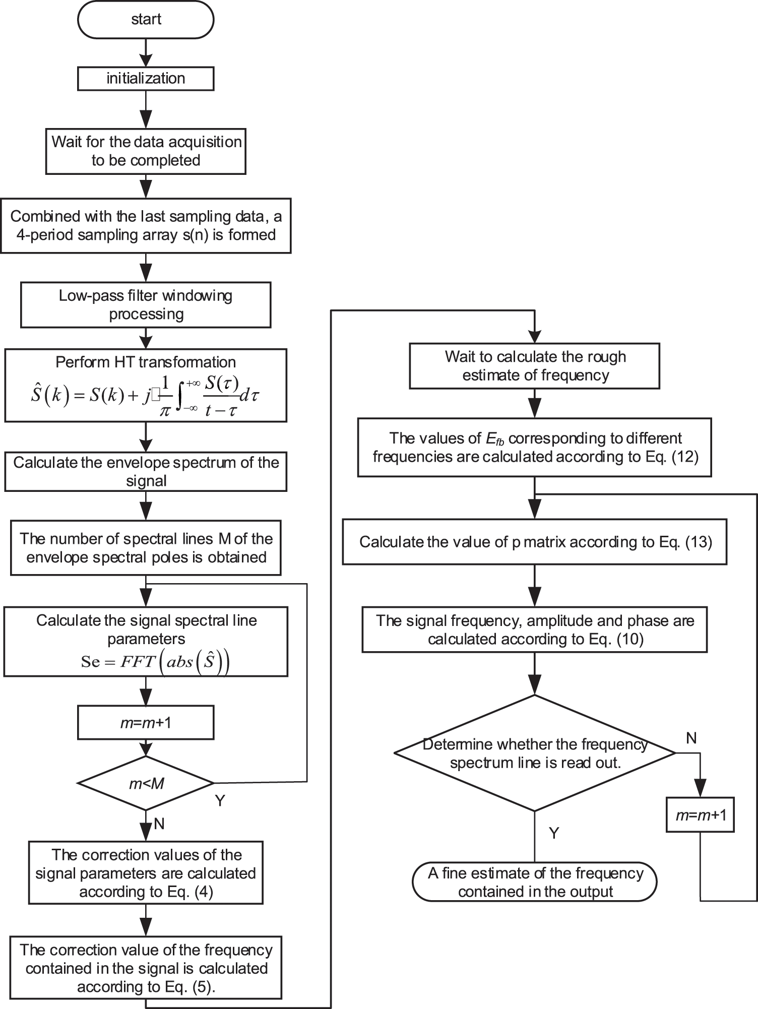
Figure 1: Algorithm flowchart of HIpST

Step 1: The collected signal s(n) is subjected to HT processing, the real data are converted into analytical data, and Fourier transform analysis is performed. The outcomes are displayed in Fig. 2. From the results of Fig. 2, it can be seen that there is no negative spectral line in the signal spectrum after HT transformation, and the amplitude of the positive spectral line becomes twice that of the original, which can reduce noise interference to a certain extent.

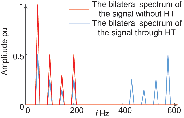
Figure 2: Frequency spectrum analysis result of signal HT

Step 2: Calculate the envelope spectrum of the signal. The envelope spectrum is sensitive to the frequency in the signal, and the total number of spectral lines M of the frequency contained in the signal is determined.

Step 3: According to the determined spectral line number b and the two adjacent spectral lines, the correction value is calculated for Eq. (4). Determine whether the number of calculations m is greater than M. If it is greater than M, the calculation is complete; otherwise, continue.

Step 4: The correction value calculated in step 3 is brought into Eq. (5) to calculate the initial value of frequency, and the coarse estimation value of frequency fb is obtained.

Step 5: Bring the results of step 4 into Eq. (11) and calculate the value corresponding to different frequencies.

Efb=[ej2π−N2NTsfb⋯0⋯0⋮⋱⋮⋮⋮00ej2π0NTsfb⋮0⋮⋮⋮⋱⋮0⋯0⋯ej2πN2NTsfb](N+1,N+1)(11)

Complex procedures on an embedded platform take a lot of time. According to the Euler rule, Eq. (11) must be divided into accessible Eq. (12) to simplify complicated procedures and shorten computation times.

Efb=diag(cos⁡(2πnNTsfb))+j⋅diag(sin⁡(2πnNTsfb))(12)

Step 6: The calculated results are brought into Eq. (13) calculation to obtain the calculated value of p, whereas a constant term, which can be completed offline, and only the values and s need to be updated each time;

p[K∗1]=(ΠHW2Π)−1ΠHW2EfbH⋅sN×1(13)

Step 7: According to the calculation results of step 5, the exact value of the signal parameters is calculated by Eq. (10). After the input data are processed by HT, the amplitude calculation formula in Eq. (10) needs to be corrected:

A=abs(p⌢(0))

Step 8: Determine whether the number of calculations m is greater than M; if it is greater than M, the calculation is completed, otherwise the calculation is continued according to steps 4–7.

4  Experimental Results and Analysis

The HIpST algorithm is optimized based on IpDFT and STWLS, focusing on the analysis of multifrequency signal parameter estimation under the superposition of noise and harmonic signals. The parameters of the proposed algorithm are set as follows: the sampling frequency is 12800 Hz, the window is 4 cycles, and the N is 1024. According to the Nyquist sampling theorem, the set sampling frequency can meet the recognition frequency of 0–6 kHz. In the implementation process of the embedded platform, when the number of calculation points is a multiple of 4, the use of the radix-4 fast Fourier transform can ensure that the calculation is completed within 500 µs. To improve the response time of the algorithm, the algorithm uses the recursive idea to update the number of sampling points in two cycles each time to ensure that the response time is 40 ms. As shown in Fig. 3.

Figure 3: Measurement data preprocessing method

The number of STWLS calculation points is odd, and the last sampling point needs to be added during the calculation. After actual testing, it does not affect the accuracy of signal estimation. To determine the effectiveness of the algorithm, three indicators are used to judge [8,19]:

TVE=(acos⁡(φ)−A0cos⁡(φ0))2+(asin⁡(φ)−A0sin⁡(φ0))2(A0cos⁡(φ0))2+(A0sin⁡(φ0))2∗100%(14)

PE=|φ−φ0|(15)

FE=|f−f0|(16)

where a is the estimated amplitude of the signal, A0 is the signal reference amplitude; φ is the phase value of signal estimation, and φ0 is the signal reference phase.

4.1 Simulation Signal Test

First, the collected signal is processed by the HT, and the real signal is converted into an analytical signal, which can expand the spectrum range and enhance the energy of the positive spectrum line under the condition of limited points. According to the basic parameter setting, the fundamental frequency range is 50 ± 0.1 Hz, and the frequency error is calculated. The results are shown in Fig. 4.

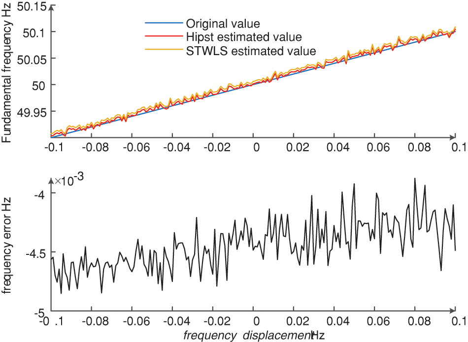
Figure 4: Influence of introducing HT on signal estimation accuracy

At the set frequency offset of −0.1–0.1 Hz, the signal is processed by HT, and the frequency estimation value and frequency error of the proposed algorithm and STWLS algorithm are calculated. The frequency error is the proposed algorithm’s estimated value minus the STWLS algorithm’s estimated value. From Fig. 4, it is clear that the fundamental frequency estimation result is closer to the real value than that without HT processing, and the maximum difference in frequency error is close to 5 mHz. Therefore, after the collected signal is processed by the HT, the improvement in the fundamental frequency estimation accuracy is 2–3 times that of the STWLS. Under the same accuracy constraints, the proposed algorithm can meet the requirements with only one calculation.

4.2 Analysis of the Accuracy of Fundamental Wave Estimation Using Different Algorithms

The TVE of the estimation results were compared when the DN signal changed dynamically to confirm the estimation accuracy of IpDFT [9], STWLS [12], and HIpST. For calculating the real voltage and current sampling per unit value, Eq. (2) replicated the voltage and current signals of the distribution network. The frequency offset was set to 50.05 Hz. The noise intensity was set to 60 dB. The harmonic was set at 100–2500 Hz, the amplitude of the maximum 10% superimposed on the fundamental signal. The estimation results of the three methods were compared, as shown in Fig. 5. When the signal amplitude modulation frequency is 0–5 Hz/s, the standard of parameter estimation is as follows: TVE is less than 0.01%. The TVE of STWLS is about 0.05%. So, the estimation results of HIpST are better than others.

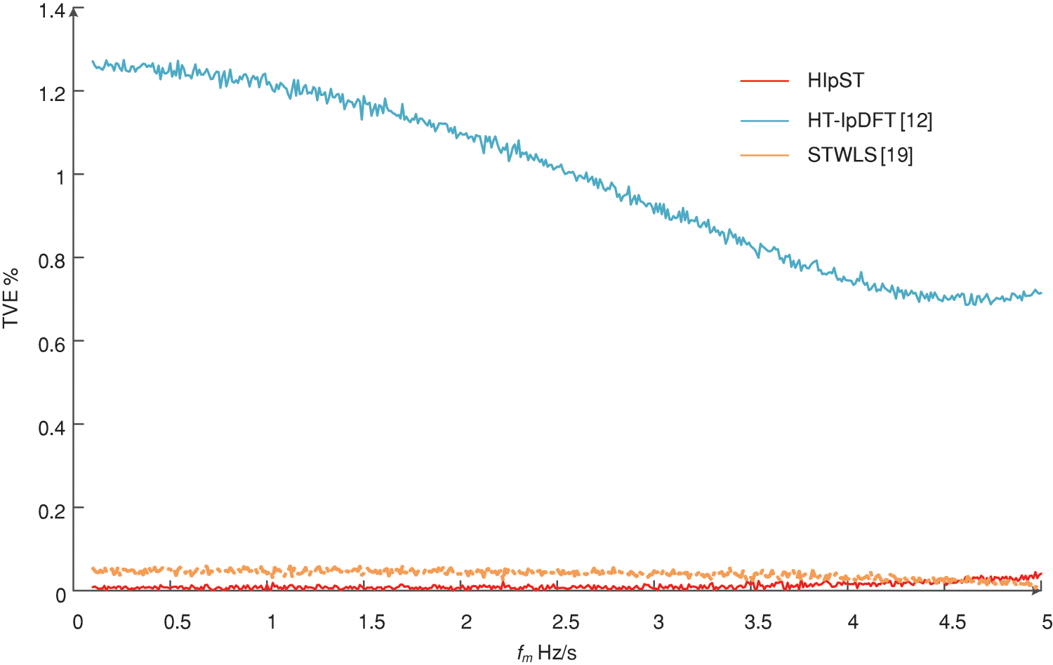
Figure 5: The TVE results of three algorithms estimate parameter estimation

4.3 Steady-State Signal Test

The steady-state signal parameters of the DN were set as follows: (1) the fundamental frequency f was in the range of 50 ± 2.5 Hz; (2) to simulate the noise interference of the signal in the actual sampling process, noise (60–80 dB) was added to the signal; and (3) harmonic (100–2500 Hz), the amplitude of the maximum 10% superimposed on the fundamental signal. The standard of parameter estimation is as follows: TVE is less than 0.1%, and FE is less than 1 mHz. The estimation results are shown in Fig. 6.

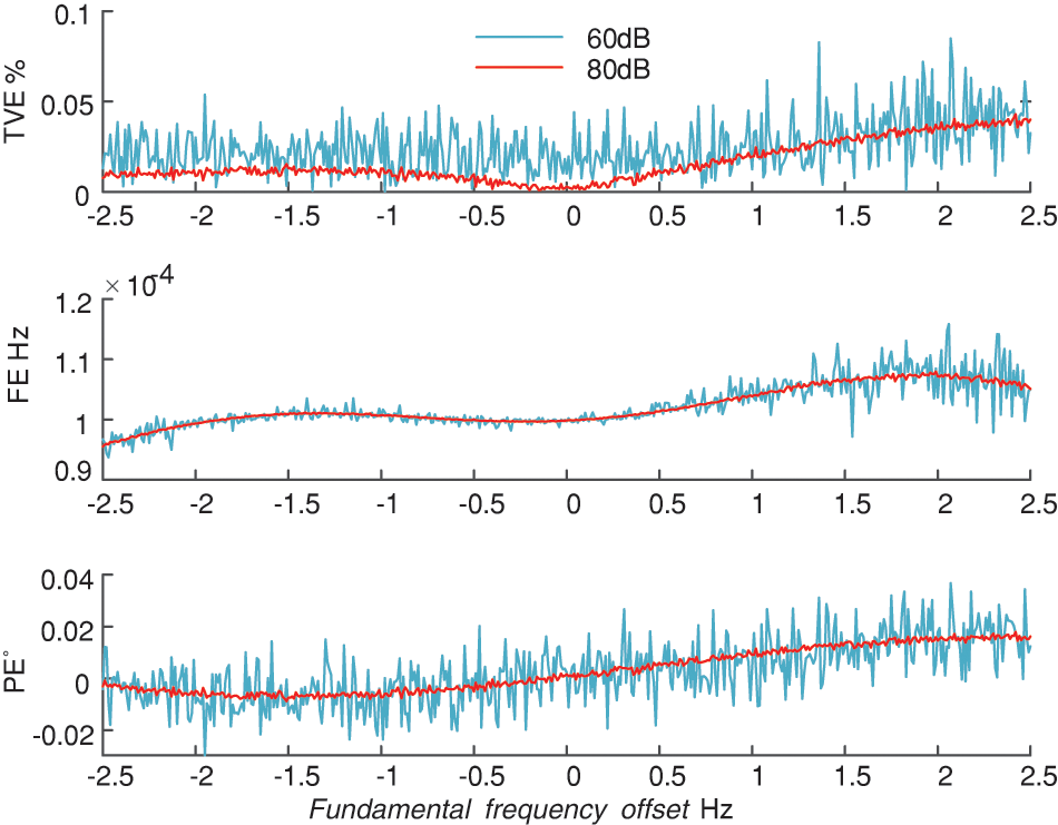
Figure 6: Parameter estimation results for a steady-state signal with harmonics

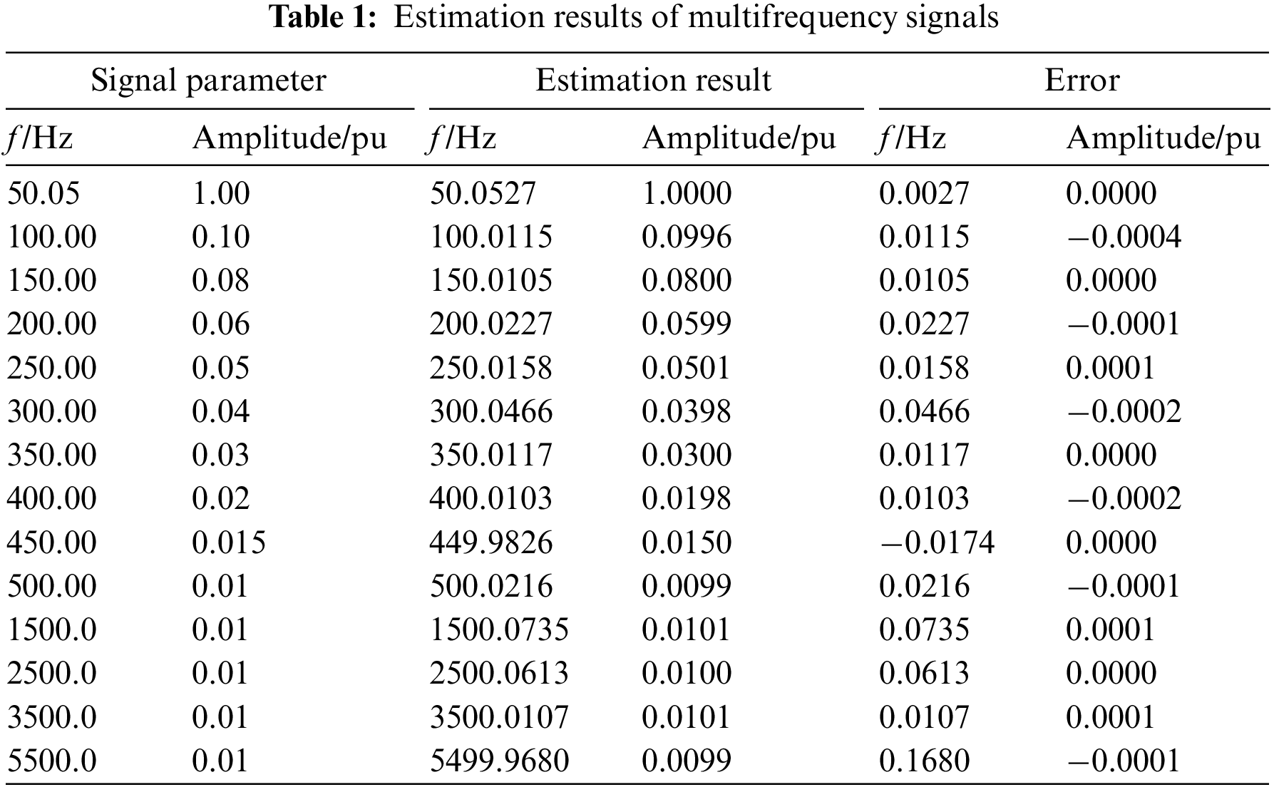
In the case of a fundamental frequency shift of −2.5–2.5 Hz, it can be observed from Fig. 6. The TVE of the proposed method is less than 0.1 %, the FE is less than 0.12 mHz, and the PE is less than 0.04°. Therefore, in the case of frequency offset and harmonics, the TVE, FE, and PE of the proposed method are far below the required limit and are not affected by the fundamental frequency offset of the signal and the existence of harmonic components.

Through the data analysis of Table 1, the amplitude error is 0.0000 pu, not that the error is zero, but due to the retention of the effective number of bits, the amplitude estimation result is relatively accurate, and the frequency estimation error is less than 100 mHz.

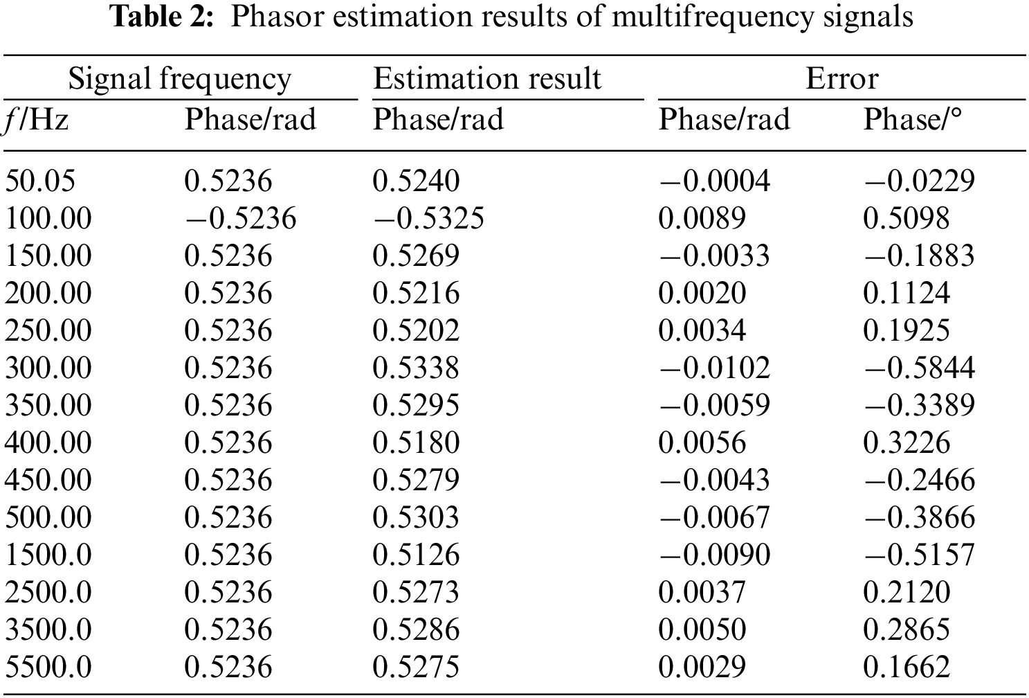
The phase of the signal model is set to −30°, the frequency is 100 Hz, and the phase of other frequency signals is set to 30°. Table 2 shows the phase estimation results of multifrequency signals. The error phase of the phase estimation results of multifrequency signals by the proposed algorithm is less than 1°, which can meet practical applications.

4.4 Dynamic Signal Test

The dynamic signal model of the distribution network was built concerning Eq. (2). The frequency offset was set to 50 ± 2.5 Hz, the modulation frequency i was set to 0.5 Hz/s, and the dynamic signal test was carried out. The noise intensity is selected between 60 and 80 dB during the test. To ensure the algorithm’s effectiveness, the noise intensity is set at 60 dB during the test. After testing, the proposed algorithm’s signal fundamental parameter estimation results are shown in Figs. 7–9. As seen from the results in Fig. 7, when the frequency offset is −2.5–2.5 Hz, the modulation frequency is 0–5 Hz/s, the signal amplitude modulation frequency is 0–5 Hz/s, and the proposed algorithm TVE is less than 1%. It can be seen from the curve that TVE increases with the gradual increase of frequency deviation and modulation frequency. When the most severe case is achieved (frequency deviation reaches 2.5 Hz, the modulation frequency is 5 Hz/s), the TVE reaches a maximum of 0.15%, still meeting the design requirements.

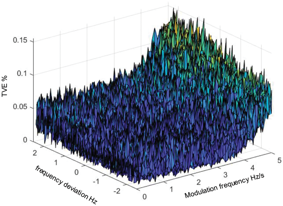
Figure 7: The TVE results of fundamental wave estimation under dynamic signals

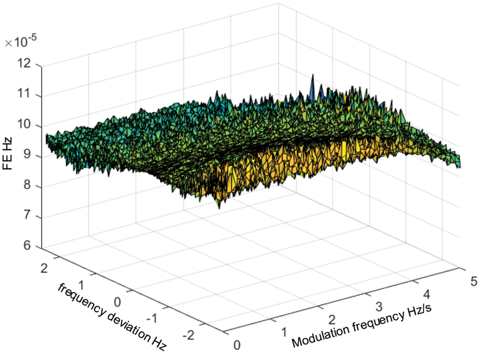
Figure 8: The FE results of fundamental wave estimation under dynamic signals

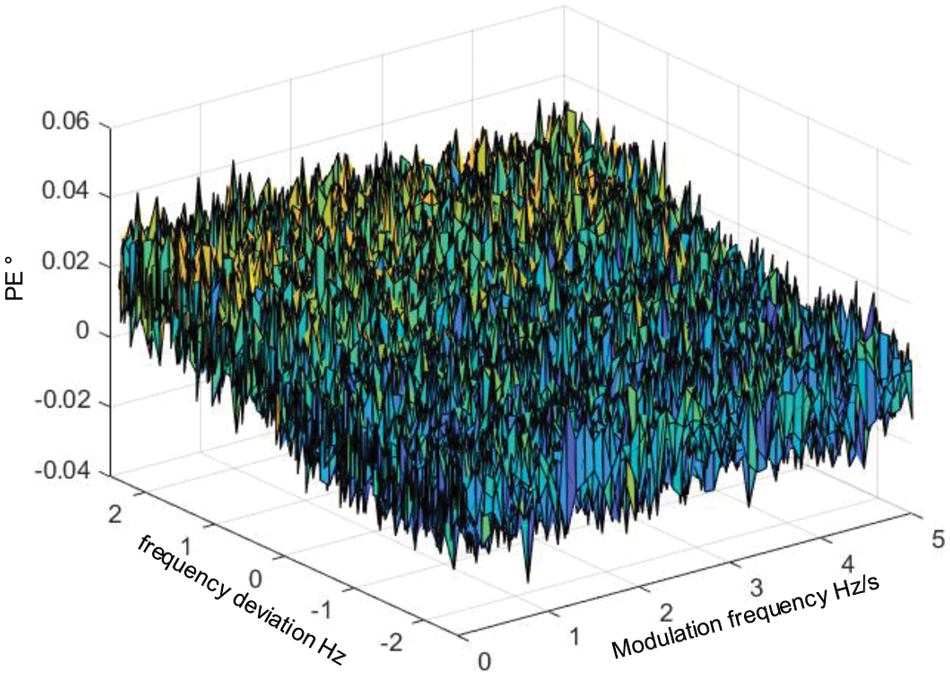
Figure 9: The PE results of fundamental wave estimation under dynamic signals

As shown in Fig. 8, when the frequency offset is −2.5–2.5 Hz, and the signal amplitude modulation frequency is 0.5 Hz/s, the frequency deviation is less than 1 mHz, which meets the design requirements. According to the fluctuation of the curve, FE gradually decreases with the frequency deviation from −2.5 to 0 Hz. With the frequency deviation from 0 to 2.5 Hz, FE is unchanged. This is because when the frequency is less than 50 Hz (−47.5–50 Hz), the signal period becomes larger, and the set data window cannot fully describe the four complete period signals. As the modulation frequency gradually increases, its FE gradually increases and reaches a maximum of 12 * 10–5 Hz in the most serious case set (frequency deviation −2.5 Hz, modulation frequency 5 Hz/s); FE still meets the design requirements.

As seen from the PE results in Fig. 9, when the frequency offset is −2.5–2.5 Hz, and the signal amplitude modulation frequency is 0–5 Hz/s, the phase error PE fluctuates little and is less than 0.1°, which can realize the dynamic estimation of the fundamental wave parameters of the distribution network signal. With the gradual increase in modulation frequency, PE is the smallest when the frequency offset is 0 Hz. With the gradual increase in the offset frequency value, PE reaches a maximum of 0.04° at the frequency offset boundary of 2.5 and −2.5 Hz.

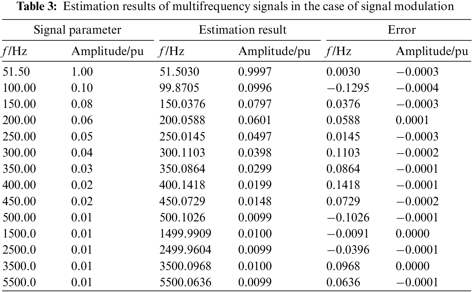
To verify the effect of the proposed algorithm on harmonic parameter estimation, the harmonic signal of 100–5500 Hz is superimposed in the signal dynamic model, and its parameters are listed in Tables 3 and 4. The estimation results of the signal amplitude and frequency are shown in Table 3. It can be seen from the results that the amplitude and frequency estimation accuracy of the fundamental wave parameters of the proposed algorithm is under the dynamic change of the fundamental wave signal.

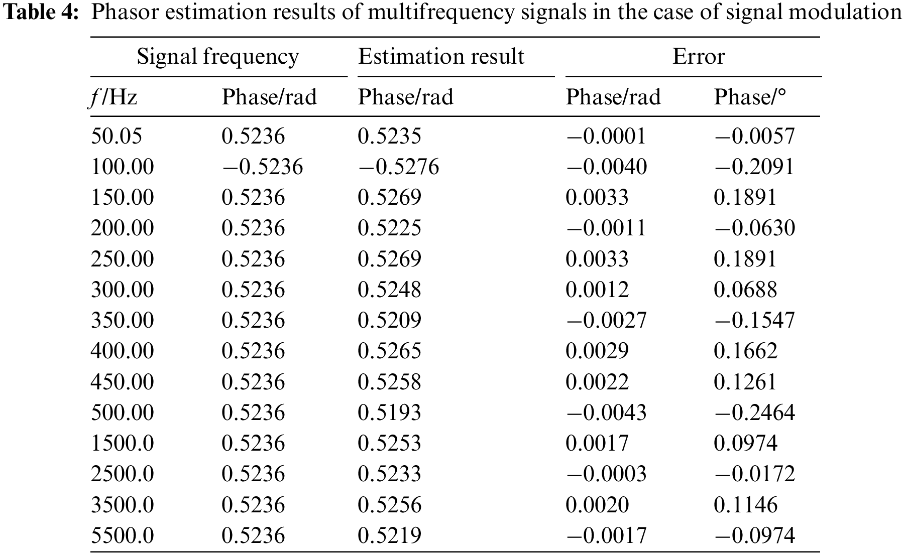
To ensure the comparability of the algorithm estimation results, the dynamic signal phase parameters are set as in Table 2. The phase estimation results of multifrequency signals are shown in Table 4. The proposed algorithm can estimate the phase of the fundamental wave parameters with high accuracy. The maximum phase estimation accuracy is less than 0.01°, and the maximum phase error of the multifrequency signal phase estimation results is less than 0.5°, which can meet practical applications. Comparing the signal phase estimation results in Tables 2 and 4, it can be seen that the phase estimation results have certain stability in static and dynamic signals.

5  Conclusion

Aiming at the strong dynamic characteristics and complex frequency components of distribution network signals, a multifrequency measurement signal estimation method for distribution networks based on HIpST is proposed. Compared with the same type of algorithm, this algorithm can realize the parameter estimation of distribution network signals and meet the existing standard requirements, which is suitable for the application requirements of different scenarios of distribution networks. Through simulation experiments, the following conclusions are drawn:

1) The proposed algorithm introduces HT, which can improve the signal frequency estimation accuracy by 2–3 times under the same calculation conditions. The proposed algorithm is still effective under different noise levels.

2) When the fundamental frequency offset is small, the estimation performance of the HIpST algorithm is more than 5 times higher than that of STWLS and HT-IpDFT. The proposed algorithm fully satisfies the 2–50 harmonic parameter estimation, and theoretically, the frequency parameter estimation below 6000 Hz can be realized.

3) Based on the multifrequency characteristics of IpDFT and the dynamic estimation advantages of STWLS, the multifrequency parameter estimation is realized based on appropriately increasing the calculation process of the algorithm, and the application scenario of the STWLS algorithm is expanded. The proposed method has the possibility of application in practical scenarios. The next research goal of the project will be to explore the application of multifrequency measurement parameters in different scenarios of distribution networks, and the deployment of synchronous measurement devices in distribution networks.

Acknowledgement: We thanked Tongliao Power Supply Company of State Grid East Inner Mongolia Electric Power Company Limited for giving financial support for this study. We would like to thank three anonymous reviewers and the editor for their comments.

Funding Statement: This project is supported by the State Grid Corporation of China Headquarters Management Science and Technology Project (No. 526620200008).

Author Contributions: The authors confirm contribution to the paper as follows: study conception and design: Bin Liu, Shuai Liang; project administration: Renjie Ding; analysis and interpretation of results: Shuguang Li; draft manuscript preparation: Bin Liu, Shuguang Li. All authors reviewed the results and approved the final version of the manuscript.

Availability of Data and Materials: The original contributions presented in the study are included in the article. Further inquiries can be directed to the corresponding author.

Conflicts of Interest: The authors declare that they have no conflicts of interest to report regarding the present study.

References

1. Rahmatian, F., Shahidehpour, M. (2021). State-of-the-art in synchrophasor measurement technology applications in distribution networks and microgrids. IEEE Access, 9, 153875–153892. https://doi.org/10.1109/access.2021 [Google Scholar] [CrossRef]

2. Mayo-Maldonado, J. C., Valdez-Resendiz, J. E., Guillen, D., Bariya, M., Meier, A. V. et al. (2020). Data-driven framework to model identification, event detection, and topology change location using D-PMUs. IEEE Transactions on Instrumentation and Measurement, 69(9), 6921–6933. https://doi.org/10.1109/tim.2020.2980332 [Google Scholar] [CrossRef]

3. Shaik, A., Praveen, T. (2018). Development of phasor estimation algorithm for P-Class PMU suitable in protection applications. IEEE Transactions on Smart Grid, 9(2), 1250–1260. https://doi.org/10.1109/tsg.2016.2582342 [Google Scholar] [CrossRef]

4. Parihar, S. S., Malik, N. (2022). Analysing the impact of optimally allocated solar PV-based DG in harmonics polluted distribution network. Sustainable Energy Technologies and Assessments, 49, 101784. https://doi.org/10.1016/j.seta.2021.101784 [Google Scholar] [CrossRef]

5. Melo, I. D., Pereira, J. L. R., Variz, A. M., Garcia, P. A. N. (2017). Harmonic state estimation for distribution networks using phasor measurement units. Electric Power Systems Research, 147, 133–144. https://doi.org/10.1016/j.epsr.2017.02.027 [Google Scholar] [CrossRef]

6. Awasthi, S., Singh, G., Ahamad, N. (2023). Identification of type of a fault in distribution system using shallow neural network with distributed generation. Energy Engineering, 120(4), 811–829. https://doi.org/10.32604/ee.2023.026863 [Google Scholar] [CrossRef]

7. Kamwa, I., Samantaray, S. R., Joos, G. (2013). Wide frequency range adaptive phasor and frequency PMU algorithms. IEEE Transactions on Smart Grid, 5(2), 569–579. https://doi.org/10.1109/tsg.2013.2264536 [Google Scholar] [CrossRef]

8. Paolo, R., Mario, P. (2014). Enhanced interpolated DFT for synchrophasor estimation in FPGAs theory-implementation and validation of a PMU prototype. IEEE Transactions on Instrumentation and Measurement, 63(12), 2824–2836. https://doi.org/10.1109/tim.2014.2321463 [Google Scholar] [CrossRef]

9. Zhan, L., Liu, Y., Liu, Y. (2018). A clarke transformation-based DFT phasor and frequency algorithm for wide frequency range. IEEE Transactions on Smart Grid, 9(1), 67–77. https://doi.org/10.1109/tsg.2016.2544947 [Google Scholar] [CrossRef]

10. Jafarpisheh, B., Madani, S. M., Shahrtash, S. M. (2016). A new DFT-based phasor estimation algorithm using high-frequency modulation. IEEE Transactions on Power Delivery, 32(6), 2416–2423. https://doi.org/10.1109/tpwrd.2016.2629762 [Google Scholar] [CrossRef]

11. Asja, D., Paolo, R., Mario, P. (2018). Iterative-interpolated DFT for synchrophasor estimation a single algorithm for P- and M-class compliant PMUs. IEEE Transactions on Instrumentation and Measurement, 67(3), 547–558. https://doi.org/10.1109/tim.2017.2779378 [Google Scholar] [CrossRef]

12. Guglielmo, G. F., Asja, D., Mario, P. (2019). Reduced leakage synchrophasor estimation: Hilbert transform plus interpolated DFT. IEEE Transactions on Instrumentation and Measurement, 68(10), 3468–3483. https://doi.org/10.1109/tim.2018.2879070 [Google Scholar] [CrossRef]

13. Ferrero, R., Pegoraro, P. A., Toscani, S. (2020). Dynamic synchrophasor estimation by extended kalman filter. IEEE Transactions on Instrumentation and Measurement, 69(7), 4818–4826. https://doi.org/10.1109/tim.2019.2955797 [Google Scholar] [CrossRef]

14. Ferrero, R., Pegoraro, P. A., Toscani, S. (2020). Synchrophasor estimation for three-phase systems based on taylor extended kalman filtering. IEEE Transactions on Instrumentation and Measurement, 69(9), 6723–6730. https://doi.org/10.1109/tim.2020.2983622 [Google Scholar] [CrossRef]

15. Bashian, A., Macii, D., Fontanelli, D., Petri, D. (2022). A tuned whitening-based Taylor-Kalman filter for P class phasor measurement units. IEEE Transactions on Instrumentation and Measurement, 71, 1–13. https://doi.org/10.1109/tim.2022.3162274 [Google Scholar] [CrossRef]

16. Bai, S., Pan, C., Xiong, S., Fu, L. (2019). A frequency estimation algorithm of power system considering out-of-band interference. Power System Technology, 43(3), 761–768. https://doi.org/10.13335/j.1000-3673.pst.2018.2766 [Google Scholar] [CrossRef]

17. Miguel, A., Jos, A. (2010). Dynamic phasor and frequency estimate through maximally Fla differentiators. IEEE Transactions on Instrumentation and Measurement, 59(7), 1803–1811. https://doi.org/10.1109/tim.2009.2030921 [Google Scholar] [CrossRef]

18. Daniel, B., Daniele, F., Dario, P. (2015). Dynamic phasor and frequency measurements by an improved Taylor weighted least squares algorithm. IEEE Transactions on Instrumentation and Measurement, 64(8), 2165–2178. https://doi.org/10.1109/tim.2014.2385171 [Google Scholar] [CrossRef]

19. Milovan, R., Žarko, Z., Božo, K. (2020). Dynamic phasor estimation by symmetric Taylor weighted least square filter. IEEE Transactions on Power Delivery, 35(6), 828–836. https://doi.org/10.1109/tpwrd.2019.2929246 [Google Scholar] [CrossRef]

20. Claudio, N., Matteo, B., Guglielmo, F., Giada, G. (2018). Fast-TFM-multifrequency phasor measurement for distribution networks. IEEE Transactions on Instrumentation and Measurement, 67(8), 1825–1835. https://doi.org/10.1109/tim.2018.2809080 [Google Scholar] [CrossRef]

21. Asja, D., Guglielmo, F., Mario, P. (2020). Beyond phasors: Modeling of power system signals using the Hilbert transform. IEEE Transactions on Power Systems, 35(4), 2971–2980. https://doi.org/10.1109/tpwrs.2019.2958487 [Google Scholar] [CrossRef]