Simulation and Analysis of Cascading Faults in Integrated Heat and Electricity Systems Considering Degradation Characteristics

1  Introduction

In recent years, the urgency to transform and upgrade the energy structure has become apparent due to the rapid growth of energy consumption and the increasing problem of environmental pollution [1]. To address these challenges, the integrated energy system (IES) has gained significant attention considering its advantages in improving energy utilization efficiency and promoting the use of renewable energy [2]. The IES has been widely regarded as the primary form of energy-carrying capacity in future society [3].

While the IES brings about positive economic and environmental benefits, it also introduces safety risks due to the coupling and impact of diverse and heterogeneous energy sources within the system [4]. An internal fault in one subsystem can propagate to other subsystems, resulting in cross-system cascading faults that endanger its overall safe operation [5,6]. As a typical application of IES, integrated heat and electricity systems (IHES) have become increasingly complex in terms of cascading faults due to the bidirectional transmission of energy flow through coupling elements. Moreover, the system components in the IHES undergo varying degrees of degradation over time and accumulate damage, which weakens their ability to withstand cascading faults. Therefore, it is crucial to comprehensively analyze the impact of system degradation on cascading faults to effectively ensure the safe and stable operation of the entire IHES.

Security is the foundation for the normal operation of an IES. Currently, a lot of research has been reported on ensuring the secure operation of power systems, with a primary focus on preventing, mitigating, and forecasting cascading faults. Wang [7] analyzed several power outage accidents caused by cascading faults and proposed preventive and emergency measures. Liu et al. [8] presented the propagation characteristics of cascading faults and developed a fault chain model for the power system. References [9,10] analyzed the impact of renewable energy integration on cascading faults in power systems. Li et al. [11] employed Long Short Term Memory (LSTM) neural networks to forecast cascading faults. Li et al. [12] utilized the arrival time of cascading faults to predict their occurrence in dynamic power grids. Nevertheless, in a tightly coupled integrated energy system comprising multiple energy sources, it is imperative to acknowledge the substantial interaction between the power system and other energy systems. References [13,14] conducted simulations to model the bidirectional cascading fault propagation process between power and natural gas systems. Fu et al. [15] examined the correlation among multiple failure modes in the IES. Liang et al. [16] conducted a risk assessment of cascading faults without taking into account the propagation path of such failures. Pan et al. [17] summarized the limitations of existing cascading fault models of IHES and proposed a fault chain search strategy considering the bidirectional coupling of electric-heating networks. Wang et al. [18] described the process of cascading faults in the IHES under extreme cold disasters using multi-time scale Markov processes.

However, the aforementioned research overlooked the performance degradation resulting from the aging of system components. Prolonged operation can lead to a decline in the efficiency of energy supply equipment and an increase in the rate of accidental failures [19]. References [20,21] indicated, through experimental measurements, that the temperature rise characteristics of transmission lines changed and the current carrying capacity limit decreased after long-term operation. References [22,23] also supported the notion that the aging of power system components escalated the risk of system interruption and diminished the reliability of energy supply. The aging and deterioration of heating pipelines are also inevitable. Vega et al. [24] analyzed the changes in adhesion strength and chemical structure of pipeline surface materials during the thermal aging process. Mazumder et al. [25] evaluated the pipeline reliability through vulnerability analysis. Research on the degradation characteristics of system components is essential for optimizing the planning and design scheme of the system [26,27], adjusting operation strategies [28], and formulating maintenance plans [19].

Based on the interaction mechanism of IHES and the electric-heating network, a cascading faults analysis method is proposed, while taking into account the degradation characteristics of the system network and equipment. By executing a numerical study, the effectiveness of the proposed method is demonstrated, and the impact of system degradation characteristics on cascading faults is revealed. The specific innovations and contributions of this research are as follows:

1) The performance degradation model of components that affect cascading faults is established, including the current carrying capacity of transmission lines, the water carrying capacity, and thermal insulation performance of thermal pipelines, as well as the degradation model of power of energy supply equipment with operation years.

2) A cascading fault simulation method for the IHES is proposed. The method adopts a fault path search strategy dominated by branch overload and considers the network island caused by branch interruption, as well as the optimal load shedding model in the case of unbalanced supply and demand in the island. Finally, the propagation and development of cascading faults are represented in the form of a fault chain.

3) The impact assessment index of cascading faults is proposed, which takes into account both network topology and load loss. The severity of cascading faults is then analyzed based on this index comprehensively.

The rest of this study is organized as follows: Section 2 introduces the interaction mechanism of the electrothermal network in the IHES and the power flow calculation method. Section 3 describes the performance degradation models of specific components. In Section 4, a cascading faults simulation method considering degradation characteristics is proposed. Section 5 introduces the numerical analysis of an IHES. The conclusions are given in Section 6.

2  Modeling and Interaction Mechanism of Electrothermal Coupling

2.1 Model of Integrated Heat and Electricity System

A typical IHES consists of a power system and a thermal system, with the two energy subsystems interconnected through coupled components such as combined heat and power (CHP) units. The thermal network and power network are composed of sources, networks, loads, and other components [29]. The power network transmits electricity via transmission lines, while the thermal network transmits heat energy through heating pipelines.

2.1.1 Power Network Model

In an IHES, the power network is divided into two models: DC and AC [30,31]. The AC model is preferred over the DC model as it takes into consideration factors such as reactive power flow and ground admittance in transmission lines. This allows for a more accurate representation of the power system’s state. Therefore, the AC model is employed in this study, which can be described as follows:

{ΔPi=Pi−Vi∑j∈iVj(Gijcos⁡θij+Bijsin⁡θij)ΔQi=Qi−Vi∑j∈iVj(Gijsin⁡θij+Bijcos⁡θij)(1)

where, ΔPi and ΔQi are the active and reactive power imbalances of node i. Pi and Qi represent the active and reactive power of node i, respectively. Vi is the voltage amplitude. G and B are conductivity and sodium. θij is the voltage phase difference between branch i and j.

2.1.2 Thermal Network Model

In a thermal network, heat is transported to the load through the heating network using a heat transfer medium and then returned to the heat source through the regenerative network, forming a closed loop. In this study, water is used as the heat transfer medium. The thermal network model consists of a hydraulic model and a thermal model [32].

The hydraulic model is used to determine the relationship between the flow rate and pressure of each pipeline in the thermal network, consisting of a continuous mass flow equation and a loop pressure drop equation:

Am=mq(2)

Bhf=0(3)

where m is the water flow rate of the pipeline. mq is the node water flow rate. A is the node-branch correlation matrix. B is the hydraulic model circuit branch correlation matrix. hf is the water pressure drop vector.

The thermal model describes the heat transfer process in a thermal network, used to calculate node temperature, heat supply, and return heat, including the thermal power equation, pipeline temperature drop equation, and mixed node temperature equation, which are shown in Eqs. (4)–(6), respectively.

Φ=cpmq(Ts−Tr)(4)

Tend=(Tstart−Ta)exp⁡(λL/cpm)+Tamb(5)

∑(mout)Tout=∑minTin(6)

where, Ts and Tr are the supply temperature and return temperature, respectively. cp is the specific heat capacity of water. Φ is the power vector of the thermal load node. Tstart and Tend are the temperatures at both ends of the pipeline, respectively. Tamb is the reference ambient temperature. min and mout represent the input and output flow rates of the pipeline, respectively. Tin and Tout represent the node mixing temperature and the temperature at the end of the injection pipeline, respectively.

2.1.3 Coupling Device Model

The coupling equipment between the electric and heating systems mainly includes CHP units, electric boilers, heat pumps, and circulating water pumps. The CHP units are the focus in this study.

A CHP unit is primarily comprised of a gas turbine and a waste heat boiler. It operates by burning natural gas to simultaneously generate electricity and heat energy. The CHP unit offers several advantages such as compact size, high controllability, low environmental requirements, and high energy utilization efficiency [33]. Depending on the energy demand of the system, the CHP unit can operate in two modes: following the electric load (FEL) and following the thermal load (FTL). The mathematical model of the CHP unit can be expressed as follows:

{cm=HCHP/PCHPPCHP=ηeGCHP(7)

where, cm is the thermoelectric ratio coefficient. HCHP and PCHP are respectively the thermal power and electrical power of the CHP unit. ηe is the power generation efficiency. GCHP is the power consumption of natural gas.

2.2 Mechanism and Analysis of Electrothermal Interaction Effects

The high level of coupling in the IHES intensifies the interaction between different components. Local fluctuations or faults can easily propagate between energy networks through coupling components, leading to a deeper propagation of faults, expanding their impact, and ultimately jeopardizing the safe and stable operation of the entire system.

The interaction among the electric-heating systems is illustrated in Fig. 1, which can be manifested as follows: Firstly, when a fault occurs in the power grid, such as a line disconnection, it disrupts the system balance. In response, the energy supply unit adjusts the generation capacity, leading to a change in the heating capacity. Secondly, the output change of the coupling unit in FEL has an impact on the thermal power of the heating network’s slack node, thus affecting the operational state of the heating network. Thirdly, changes in the operating state of the heating network will, in turn, affect the power system through the coupling unit in FHL. The same principles apply to faults occurring in the heating network.

Figure 1: Schematic diagram of the interactive effects of the electric-heating network

Overall, the interaction between electric-heating systems is accomplished through the transmission of coupling components. When a disturbance arises in one system, it propagates to other systems via coupling elements, thereby affecting the original system. Therefore, when evaluating the overall operational status of a system, it is crucial to comprehensively consider the operational status and response characteristics of multiple systems.

The operational status of IHES can be quantitatively analyzed through power flow calculations. Currently, two commonly used power flow calculation methods are the unified method and the decomposition method. The decomposition method is preferred due to its advantages including lower model dimensions, faster solving speed, and higher flexibility [34,35]. As a result, it has been employed for solving the system power flow through alternating iterations, as depicted in Fig. 2.

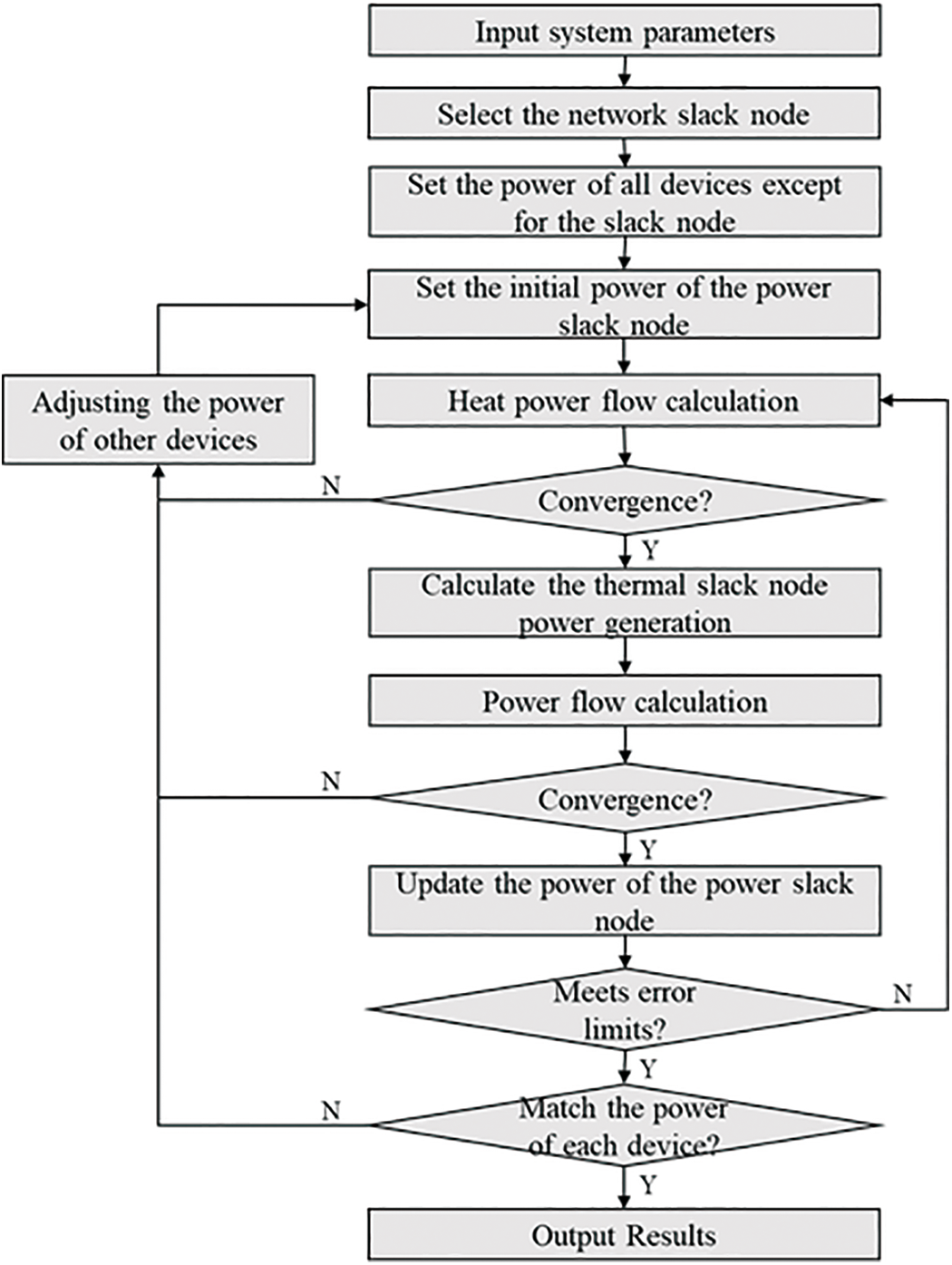
Figure 2: Flow chart of power flow calculation for IHES

3  The Degradation Model of IHES

3.1 Degradation Model of Electric-Heating Network

3.1.1 Transmission Line

Transmission lines are considered the most susceptible component of the power system, with line overload being the most prevalent type of fault [36]. The current carrying capacity of a transmission line depends on its maximum allowable operating temperature. A higher allowable temperature results in a greater current-carrying capacity. During operation, the primary sources of heat in transmission lines are the thermal effect of current and the absorption of solar radiation. Heat dissipation methods mainly involve convective heat dissipation and radiation heat dissipation. The calculation method for determining the current-carrying capacity of a wire can be expressed using the heat balance equation. According to the heat balance equation, the calculation method for the current carrying capacity of a wire can be expressed as:

I=(WR+WF−WS)R(TC)(8)

where, WR, WF and WS represent radiative heat dissipation power, convective heat dissipation power, and solar heat absorption power per unit length of wire, respectively. The specific calculation formula is shown in IEEE Standard [37]. TC is the wire temperature, and R(TC) is the AC resistance of wire at TC temperature.

According to the heat balance equation, the current carrying capacity of a transmission line is determined by the maximum real-time power flow value at the maximum allowable operating temperature. This power flow value is denoted by PR, and it is calculated using Eq. (9). If the current flowing through the line exceeds this calculated value, the line will overheat, resulting in disconnection.

PR=g(I(TC))(9)

As the operating time of a transmission line increases, the surface roughness of the line also increases, and pollutant layers start to accumulate. These factors have a negative impact on the heat dissipation performance of the wire. Additionally, the tensile strength of aging lines decreases, and the resistance per unit length increases [21]. These factors not only affect the temperature rise characteristics of the wires but also result in increased power transmission losses, reducing overall economic efficiency [23]. Consequently, the maximum allowable operating temperature of the transmission line decreases, leading to a decrease in its current carrying capacity. This makes the line more susceptible to overload, especially during periods of peak electricity consumption.

Eqs. (8) and (9) show that the calculation of the current carrying capacity of aging lines needs to comprehensively consider factors such as temperature, conductor wear and corrosion, insulation condition, and damage to supports and insulators. The degradation of current carrying capacity is intricately linked with the material characteristics and working conditions of the conductor. By incorporating the material characteristic coefficient and operating environmental coefficient, the functional relationship between the current carrying capacity of transmission lines and the increase in operating years can be simplified as follows:

PR(t)=PR0(1−δatδe)(10)

where, t is the operating years. PR0 is the current carrying capacity of the transmission line in a brand-new state. δa is the material property coefficient of the line. δe is the operating environment coefficient, which is related to the time of the wire in a high-temperature environment.

3.1.2 Heating Pipeline

During the operation of a thermal pipeline, various factors such as uneven water temperature, chemical corrosion, and impurity deposition affect the inner wall of the pipeline, leading to the formation of rust and scale. This results in a reduction in the effective inner diameter of the pipeline and subsequently decreases its water delivery capacity [38]. Additionally, the roughness of the inner wall of the pipeline increases, causing an increase in head loss. The Hazen-Williams formula is commonly used in many countries for hydraulic calculations of water supply pipelines [39]. By adjusting the coefficients of the Hazen-Williams formula, hydraulic calculations can be performed on pipelines with different roughness coefficients:

hf=10.67q1.852Chw1.852d4.87l(11)

where, q is the design flow. Chw is the coefficient of the Hazen-Williams formula. d is the pipe diameter. l is the pipe length.

Previous research has indicated that the value of Chw exhibits a characteristic of varying with operating years [40]. Consequently, the degradation model for the water delivery capacity of pipelines can be inferred from the changes in this value. Since water supply networks often comprise pipes with different diameters, and the pipe diameter is a significant factor influencing the value [41], it becomes essential to establish a functional relationship between the value Chw, pipe diameter, and operating years. Representative cast iron pipes with different laying years, diameters, and locations in a certain water supply network are selected for Chw value testing, and the results are shown in Table 1 [42].

By executing regression analysis, the functional equation for the value Chw of cast iron pipes can be obtained as follows:

Chw(d,t)=0.0031d1.0119+257.537e−0.0053t−128.7514(12)

Moreover, the insulation layer on the surface of thermal pipelines may undergo material aging, structural changes, and other issues over time due to environmental and operating conditions. This deterioration in insulation performance results in increased heat loss within the pipeline network. The degradation of insulation performance is influenced by factors such as thermal conductivity, eccentric structure, and hollow structure. Specifically, the primary cause is the increase in thermal conductivity [43,44]. The relationship between thermal conductivity and operating years can be expressed as follows:

λ(t)=λ0(1+γt)(13)

where, λ0 is the initial thermal conductivity and γ is the annual average growth rate.

3.2 Equipment Degradation Model

As service time increases, the equipment within the system inevitably undergoes a degradation process in performance. This is caused by the gradual accumulation of wear and aging of the internal electrical and mechanical components after prolonged operation. The degradation rate is especially accelerated for equipment operating under high loads and in harsh external environments. The degradation of equipment performance is manifested by a decrease in output capacity, efficiency, and an increase in heat rate, resulting in a decrease in the equipment’s energy supply capacity and reliability. The aging of equipment within the IHES impacts the system’s operational status and optimization scheduling outcomes.

The degradation trajectory model is a mathematical representation that describes how equipment degradation changes over time as it operates. This model takes into account factors such as operating time, load, environmental conditions, and maintenance practices to estimate the rate at which equipment performance deteriorates. By using this model, the current state of equipment degradation can be understood, the informed decisions about maintenance and replacement strategies can be made. The variation of equipment degradation ΔF with operating time can be represented as:

ΔF=f(t,β,ε)+τ+i0(14)

where, f is a degenerate function, commonly available in two types: linear and exponential. β is the constant parameter in the degenerate function. ε is the random parameter of the degradation function, which is related to random effects. τ is the degradation caused by sudden faults. i0 is the initial wear and tear of the equipment.

As a coupling element connecting the electrical and thermal networks, the CHP unit is the core component of an IHES. Actually, the CHP unit is not a single piece of equipment, but a combined system including power generation and heat recovery devices. Among these, the prime mover is the core device within a CHP system. Obviously, besides the prime mover, the auxiliary equipment (waste heat boilers, steam or hot water generators, etc.) of the CHP system such as may also degrade over time. Nonetheless, given the significance of the prime mover within a CHP unit, the degradation characteristics specifically related to the prime mover are focused in this study. Moreover, considering its wide application in the IHES especially for regional applications, the gas turbine is assumed as the prime mover of the CHP system.

Blade fouling is a significant cause of overall performance degradation in gas turbines [45]. This degradation is primarily caused by the corrosion of blades due to impurities and particles present in the air, as well as the scaling of oil and gas. These factors lead to a reduction in the inlet flow rate of the compressor and a decrease in the unit’s efficiency. The scaling on compressor blades is a form of recoverable degradation that can be addressed through maintenance measures such as cleaning and maintenance. However, corrosion and wear of components result in irreversible degradation [46], leading to a decline in overall performance as the equipment ages.

In general, the degradation function of a gas turbine can be expressed in the exponential form [47], and its degradation model can be expressed as Eq. (15). The exponential degradation function demonstrates that the rate of degradation in gas turbines gradually decreases over time. By measuring and monitoring the performance parameters of gas turbines, it is possible to estimate the parameters in the degradation model.

ΔF=eβ⋅tε+τ+i0(15)

For thermal power generation units, the basic aging coefficient Bf of the equipment can be obtained using Eq. (14). The calculation of aging coefficient PFi can refer to the estimation formula provided by the American Society of Mechanical Engineers (ASME):

PFi=Bflg⁡W0p0po′(16)

where, W0 is the rated power. p0 and p0′ are the inlet pressure of the steam turbine and the inlet pressure of the steam turbine at rated load, respectively.

The expression for the PF of the entire unit is obtained by weighting each equipment of the unit:

PF=∑i=1n(PFi⋅Si)∑i=1nSi(17)

where, n is the number of equipment inside the unit. Si is the corresponding weight coefficient.

4  Simulation Method for Cascading Faults Considering Degradation Characteristics

4.1 Fault Path Search Strategy

During the evolution and development of cascading faults, one common form of propagation is branch disconnection caused by overload [8,17,48]. In this study, the impact of trend changes on cascading faults is specifically focused on an overload-dominated development model utilized to predict the propagation path of cascading faults. There exists a clear causal relationship between the preceding and subsequent faults in the overload-dominated cascading fault. The preceding fault alters the system network structure and power flow operating conditions, thereby triggering the subsequent fault.

In the study of cascading faults in the IHES, it is important to note that the propagation process of these faults is often gradual. Therefore, the static analysis methods are primarily utilized to investigate the cumulative effects of faults that have occurred, the impact of single faults, system bearing capacity, and other factors that affect the stability of the system [49]. The cascading fault path is represented by connecting successively overloaded branches, highlighting the sequence of branch disconnections.

In this study, the scenario considered involves a single branch being disconnected, which acts as the initial triggering fault. The fault development is then simulated after all branches are disconnected using an enumeration method. When cascading faults occur, a fault chain is generated and an impact assessment is conducted.

To simulate the fault development after all branches are disconnected, the following steps can be followed:

Step 1. Set a branch disconnection as the initial triggering fault: Choose a branch in the network and disconnect it to initiate the fault.

Step 2. Update the network topology: After the branch disconnection, update the network topology to reflect the changes. This may lead to the system being decomposed into multiple sub-networks.

Step 3. Evaluate the energy supply capability of sub-networks: For each sub-network, evaluate whether there is sufficient energy supply equipment to meet the load demand. If there is an insufficient energy supply, that sub-network will need to be shut down, resulting in the loss of all loads within it. If energy supply equipment is available, it is important to assess whether it can meet the load demand considering capacity configuration and aging issues. In the event of a supply-demand imbalance, certain loads may require active disconnection using an electric-heating scheduling model to maintain balance within the sub-network.

Step 4. Recalculate network flow: If the load demand can be met within the sub-network, designate a new slack node and recalculate the network flow to incorporate the modifications in the network topology and load distribution.

Step 5. Identify overloaded branches: As the network’s carrying capacity diminishes due to branch disconnections, there is a higher probability of branches becoming overloaded. Identify the branches that are overloaded and at risk of failure under the existing conditions.

Step 6. Select subsequent fault: When a single branch is overloaded, it should be cut off as a subsequent fault. However, in cases where multiple branches are overloaded, cutting off all of them can heighten the risk of system collapse and undermine the significance of conducting cascading fault analysis. Therefore, it is crucial to select a single line for disconnection as a subsequent fault, considering the propagation distance of cascading faults.

Step 7. Repeat steps 2 to 6: Continue updating the network topology, assessing energy supply capability, recalculating network flow, identifying overloaded branches, and selecting subsequent faults until there are no more overloaded branches in the system.

Step 8. Calculate load loss and output fault chain: After completing the fault development process, calculate the load loss in each sub-network and generate the fault chain, which illustrates the sequence of faults that occurred during the cascading process.

In summary, the specific simulation process is shown in Fig. 3.

Figure 3: Cascading faults simulation flowchart considering degradation characteristics

4.2 Electric-Heating Joint Scheduling Model

The primary objective of operating an integrated energy system is to meet the load demand while ensuring safety and stability. In the event of a cascading fault within the system, where energy supply in a specific sub-network fails to meet demand, load-shedding measures must be implemented to restore supply-demand equilibrium and minimize losses through efficient scheduling.

Taking into account the varying energy qualities of electricity and heating, a conversion factor known as the energy quality coefficient φ is introduced. The energy quality coefficient φelec for electrical load is defined as 1, while for thermal load, the energy quality coefficient φheat is calculated as follows:

φheat=1−TambTheat(18)

where, Theat is the temperature for the heat load.

The electric-heating joint scheduling model should consider both minimizing load losses and minimizing the output adjustment of energy supply equipment. The objective function can be expressed as:

min[∑i∈NDφPcr,i+ω∑j∈NGΔWj](19)

where, ND and NG represent the number of load shedding nodes and energy supply equipment, respectively. Pcr,i is the load-shedding capacity of the node i. ΔWj is the output adjustment of equipment j. ω is the weight coefficient, generally taken as 0.1.

The constraints that need to be met during the scheduling process include the following:

1) Power balance constraints, including node power balance and system power balance:

∑k=1NkPk=0(20)

∑i∈NLPLi+Pc,loss=∑j∈NGWj(21)

where, Nk is the total number of branches connected to node i. Pk is the power of the k-th branch, defined as positive power inflow and negative power outflow. NL is the load aggregation. PLi and Wi are the power of unit and node loads, and Pc,loss is the total network loss.

2) Unit output constraints:

Wi,min≤Wi≤Wi,max(22)

where, Wi,max and Wi,min refer to the upper and lower limits of the unit’s output, respectively.

3) Transmission constraints:

Sk,min≤Sk≤Sk,max(23)

where, Sk represents the power flow of the branch k, with line transmission power in the power grid and pipeline flow in the heating network. Sk,max and Sk,min are the upper and lower limits of the branch flow, respectively.

4) State variable constraints:

xn,min≤xn≤xn,max(24)

where, xn is the system state variable, mainly including grid node voltage, phase angle, and heating network node temperature, pressure, etc. xn,max and xn,min represent the upper and lower limits of the system state variables, respectively.

5) Load shedding constraint:

0≤Pcr,i≤Pcr,imax(25)

where, Pcr,max is the load shedding upper limit of the node i.

4.3 Fault Impact Assessment

To assess the impact of cascading faults on the system, both load loss and structural loss are considered in this study as metrics.

The load loss encompasses the load in the forced closed sub-network and the load cut through scheduling. It is calculated by dividing the sum of these two loads by the total load, as shown in Eq. (26).

ΔPloss=∑Pclose+∑Pcr∑PLi(26)

where, ΔPlossp is the load loss rate. Pclose is the load within closed sub-networks.

The structural loss reflects the impact of cascading faults on the topological integrity of the system. It is measured through the calculation of system integrity, which considers both power grid integrity and heat grid integrity. System integrity is defined as the ratio of the maximum number of nodes in the operating sub-network to the total number of nodes, as shown in Eq. (27).

Rs=Ns,maxN(27)

where, Rsp is system integrity. Ns,max is the maximum number of nodes contained in the running sub-network. N is the total number of nodes in the system.

5  Numerical Study

5.1 Introduction of the Test System

In this study, an improved IEEE14-node power system [17] and a 13-node thermal system [16] are employed as an example for simulation analysis. The system structure is shown in Fig. 4. ei and hi represent the electric heating load nodes, respectively. pi is the heating pipeline, and bi is the transmission line. The system includes two CHP units and two conventional thermal power generation units. The CHP1 unit is connected to the node h13 and e3, and the CHP2 unit is connected to the node h12 and e1. Grid nodes e2 and e6 are connected to the generator. The total heat load is 2.1 MW, and the total power load is 2.29 MW. When the system is operating normally, e1 is the grid slack node and h13 is the slack node of the heating network.

Figure 4: Structure diagram of the analyzed IHES

5.2 Degradation Parameters and Scenario Setting

To investigate the influence of system degradation on cascading faults, four scenarios are assumed for comparative analysis:

Scenario 1: The system has just been put into operation and does not consider degradation characteristics as the baseline scenario.

Scenario 2: A general aging system that has been in operation for 10 years.

Scenario 3: A severely aging system that has been in operation for 20 years.

Scenario 4: A severely aging system that has been in operation for 30 years.

In each scenario, the running time of equipment, pipelines, and other system components is set to be the same.

The widely used LGJ-type transmission line is selected, and the degradation curve obtained from Eq. (10) is illustrated in Fig. 5. According to the curve, the degradation level of the transmission line after 25 years and 35 years of operation is found to be 93.35% and 87%, respectively. These values are in good agreement with the findings reported in [49].

Figure 5: Degradation curve of transmission line carrying capacity

In the analysis of the hot water pipeline, a universal cast iron pipeline is chosen. The degradation characteristics of its water delivery capacity and insulation performance are calculated using Eqs. (12) and (13), respectively. Moreover, it is assumed that the average annual growth rate of thermal conductivity for cast iron material is 1.37% [32].

Considering the complexity of the CHP unit, the degradation characteristics of the gas turbine are employed as a simplified representation. These characteristics can be calculated using Eq. (15). Furthermore, the aging coefficient of the generator can be computed using Eqs. (16) and (17).

5.3 Results and Discussion

5.3.1 Comparative Analysis of Cascading Faults under Different Aging Degrees

The concept of cascading fault path is defined as a sequence of n consecutive fault links, which is referred to as an n-order cascading fault. In Fig. 6, the number of cascading faults with different orders in four scenarios is illustrated. It can be observed that as the system operates for a longer duration and experiences deeper degradation, the frequency of cascading faults increases gradually. Taking p3 as the initial triggering fault for example, in Scenario 1, it cannot trigger a cascading fault. However, with the continuous degradation of the system, a 2-order fault chain of “p3→p8” is formed in Scenario 2. In Scenario 4, the cascading fault further evolves and expands, resulting in a 3-order fault chain of “p3→p8→b3”. Simultaneously, the increase in the order of fault chains indicates that system degradation leads to a higher probability of branch overload, making it easier to form high-order cascading faults.

Figure 6: Number of fault chains under different scenarios

The load loss rate caused by cascading faults under different scenarios is illustrated in Fig. 7. The load loss rate consists of two components: the node load in the sub-network that is forced to shut down and the active load removal through scheduling. In some cases, certain cascading faults may lead to the same load loss rate across different scenarios. This phenomenon occurs because the load loss is primarily attributed to the node load of the forced closed sub-network. As the system ages and experiences degradation, some sub-networks may be forced to shut down, resulting in a loss of load. However, the remaining sub-networks can still operate normally. Therefore, the load loss remains unchanged in these cases as the system degrades.

Figure 7: Load loss rates under different scenarios

The situation of an increased load loss rate can be categorized as follows. The first type is represented by the chain fault formed by initial triggering faults in branches b1, b4, and b18. In subsequent scenarios, the fault chain remains unchanged. The increase in load loss is primarily attributed to the system’s degradation, leading to a decrease in network carrying capacity and equipment energy supply capacity. To ensure the safe operation of the system, there is an increased need to actively cut off loads through the scheduling model. It is important to note that the equipment, transmission lines, and thermal pipelines in the system have been in operation for 30 years and are approaching the end of their service life in Scenario 4. Consequently, the rate of performance degradation is much higher compared to the past, resulting in a significant increase in the load loss rate. The second type is caused by the addition of fault chains, such as the disconnection of branch b12 until Scenario 3. This can lead to cascading faults and load loss, although not all new fault chains necessarily result in load loss. The third type is characterized by changes in the path of cascading faults, which may divide the system into new sub-networks. This division increases load loss within the sub-networks and requires an increased load cutoff through electric heating scheduling, thereby resulting in a significant rise in the load loss rate.

5.3.2 Analysis of Cascading Faults without Considering Degradation Characteristics

Based on the aforementioned comparative analysis, an in-depth analysis of cascading faults is conducted before and after considering degradation characteristics. In Scenario 1, the results of cascading faults without considering degradation characteristics are shown in Table 2. Eight cascading fault chains are identified, with two being high-order fault chains (4th order and above), accounting for 25% of the total. By analyzing the impact of these cascading faults, it is found that the average load loss rates generated by all cascading fault chains in Scenario 1 are 0.1542 (electrical) and 0.1420 (thermal), with the average system integrity measured at 0.9107 (electrical) and 0.9135 (thermal). Overall, the impact on the system is relatively low. However, there are instances where the low-order fault chain “p5→p3” has a significant impact. This is due to both branches, p5, and p3, serving as main lines of the heating network. The disconnection of branch p5 forced the CHP2 unit offline, resulting in a decrease in the system’s energy supply capacity. Similarly, the disconnection of branch p3 divided the heating network into two parts, leading to a lack of energy supply equipment in the lower half of the sub-network, causing a significant loss of load and a corresponding reduction in the integrity of the heating network.

5.3.3 Analysis of Cascading Faults Considering Degradation Characteristics

In Scenario 4, which represents the system with the longest running time and the deepest degree of degradation, a simulation considering the system’s degradation characteristics is executed. The results, as shown in Table 3, indicate a significant increase in the number of cascading fault chains from 8 (in Scenario 1) to 15. This suggests that the degradation of the system reduces the load-carrying capacity of the network, weakens its resistance to network disturbances, and increases the likelihood of cascading faults.

The increase in the proportion of high-order fault chains indicates that the degradation characteristics of the system can lead to more complex and extensive cascading faults. This highlights the importance of considering degradation in analyzing and managing the resilience of the IHES. For example, the 3rd-order fault chain “b7→b3→b20” demonstrates how degradation can influence the development of cascading faults. Without considering degradation, the fault chain would terminate at branch b20, and the system would reach stability without any overloaded branches. However, with degradation, the decrease in network carrying capacity leads to branch b6 becoming overloaded, which further propagates the cascading faults. In addition, the degradation can also affect the direction of cascading faults. In the case of the cascading faults caused by the opening of branch b17, considering degradation leads to the next order fault changing from branch b14 to branch b11. This change is based on the system topology and power flow transfer, as the priority of disconnecting branch b11 is higher when both branches b11 and b14 are overloaded.

From the perspective of the severity of the impact of cascading faults, the average load loss rate of the 8 initial fault chains with the same initial triggering faults as Scenario 1 in Scenario 4 increases to 0.2358 (electrical) and 0.2333 (thermal). Additionally, the system integrity decreases to 0.8393 (electrical) and 0.8624 (thermal), indicating that system degradation significantly exacerbated the impact of cascading faults. However, not all cases of load loss will increase, as it depends on the underlying causes. The increase in load loss can be attributed to two factors: firstly, an escalation in chain failures leading to load loss, and secondly, a decline in energy supply capacity due to equipment performance degradation. Taking the cascading fault chain “b13→b16→b14” as an example, the load loss, in this case, is attributed to the absence of energy supply equipment in the isolated islands of nodes e13 and e14. When considering the degradation characteristics, the fault chain remains unchanged, therefore the load loss will not increase. Similarly, in the chain fault with branch b11 as the initial trigger fault, the load loss decreases when considering the degradation characteristics. The reason is that in Scenario 1, the cascading fault causes the CHP2 unit to shut down, resulting in a substantial amount of load loss. In Scenario 4, the cascading fault path changes, allowing the CHP2 unit to supply energy normally, thus leading to reduced load loss. The decrease in system integrity is attributed to system degradation, which extends the chain of cascading faults, resulting in more severe damage to the system structure. This is closely related to the specific details of the evolution and development of cascading faults.

6  Conclusions

To thoroughly explore the impact of degradation characteristics on the cascading faults of the IHES, after developing a system component degradation model, a simulation method for cascading faults dominated by overload type is proposed. The propagation of cascading faults is depicted in the form of fault chains. By conducting a simulation analysis of an illustrative example, the following conclusions are drawn:

(1) After considering the degradation characteristics of system components, the frequency and severity of cascading failures caused by a single branch disconnection increase due to the decrease in network carrying capacity, significantly elevating the risk of cascading failures.

(2) Aging circuits are more vulnerable to overload, which can affect the progression of chain failures. This impact is manifested in two ways: an increase in the order of the fault chain and a change in the direction of chain failure propagation.

(3) When comparing the occurrence of cascading faults in systems with varying degrees of aging, it becomes evident that systems with severe aging are more susceptible to large-scale cascading failures. Therefore, timely replacement and maintenance of aging components are crucial to ensuring the safe operation of the system.

During the development of cascading faults, random faults resulting from branch disconnections and changes in the system state are also important factors that contribute to the progression of cascading faults. System degradation can also influence random faults, necessitating further research in the future. Moreover, as to the equipment degradation, besides the prime mover, the analysis of degradation characteristics of other auxiliary equipment within a CHP unit is expected to be included in the following studies, to grasp the degradation characteristics of coupled devices more comprehensively. In addition, while considering the relatively small scale of the IHES, the enumeration method has been employed to simulate fault development. However, as to some large-scale IHES, while considering the computational burden, the sampling method may be a choice.

Acknowledgement: None.

Funding Statement: The research work was supported by Shanghai Rising-Star Program (No. 22QA1403900), the National Natural Science Foundation of China (No. 71804106) and the Non-carbon Energy Conversion and Utilization Institute under the Shanghai Class IV Peak Disciplinary Development Program.

Author Contributions: The authors confirm contribution to the paper as follows: study conception and design: H. Cui and H. Ren; data collection: Q. Wu and W. Zhou; analysis and interpretation of results: Q. Li; draft manuscript preparation: H. Cui and H. Ren. All authors reviewed the results and approved the final version of the manuscript.

Availability of Data and Materials: All data, models, or codes that support the findings of this study are available from the corresponding author upon reasonable request.

Conflicts of Interest: The authors declare that they have no conflicts of interest to report regarding the present study.

References

1. Mohy-ud-din, G., Vu, D. H., Muttaqi, K. M., Sutanto, D. (2019). An integrated energy management approach for the economic operation of industrial microgrids under uncertainty of renewable energy. IEEE Transactions on Industry Applications, 56(2), 1062–1073. [Google Scholar]

2. Tahir, M. F., Chen, H. Y., Han, G. Z. (2021). A comprehensive review of 4E analysis of thermal power plants, intermittent renewable energy and integrated energy systems. Energy Reports, 7, 3517–3534. [Google Scholar]

3. Li, Z., Wang, C. F., Li, B., Wang, J. Y., Zhao, P. H. et al. (2020). Probability-interval-based optimal planning of integrated energy system with uncertain wind power. IEEE Transactions on Industry Applications, 56(1), 4–13. [Google Scholar]

4. Wang, K., Wang, C. F., Zhang, Z. W., Dong, X. T., Jiang, F. (2021). Multi-timescale active distribution network optimal dispatching based on SMPC. IEEE Transactions on Industry Applications, 58(2), 1644–1653. [Google Scholar]

5. Li, H., Hou, K., Xu, X. D., Jia, H. J., Zhu, L. W. et al. (2022). Probabilistic energy flow calculation for regional integrated energy system considering cross-system failures. Applied Energy, 308, 118326. [Google Scholar]

6. Sun, Q. Y., Yang, L. (2019). From independence to interconnection–A review of AI technology applied in energy systems. CSEE Journal of Power and Energy Systems, 5(1), 21–34. [Google Scholar]

7. Wang, J. N. (2019). Power grid cascading failure blackouts analysis. AIP Conference Proceedings, 2066(1), 020046. [Google Scholar]

8. Liu, Y. M., Wang, T., Guo, J. Y. (2022). Identification of vulnerable branches considering spatiotemporal characteristics of cascading failure propagation. Energy Reports, 8, 7908–7916. [Google Scholar]

9. Yang, S. H., Chen, W. R., Zhang, X. X., Yang, W. Q. (2020). A graph-based method for vulnerability analysis of renewable energy integrated power systems to cascading failures. Reliability Engineering and System Safety, 207, 107354. [Google Scholar]

10. Liu, D., Zhang, X., Tse, C. K. (2022). Effects of high level of penetration of renewable energy sources on cascading failure of modern power systems. IEEE Journal on Emerging and Selected Topics in Circuits and Systems, 12(1), 98–106. [Google Scholar]

11. Li, D. H., Wang, Q., Zhang, X., Fan, X. J. (2023). Predicting the cascading failure propagation path in complex networks based on attention-LSTM neural networks. 2023 IEEE International Symposium on Circuits and Systems (ISCAS), pp. 1–4. Monterey, USA. [Google Scholar]

12. Li, B. B., Jia, A. H., Chen, L. F. (2022). A prediction model towards the cascading failure of power grids. 2022 12th International Conference on Power and Energy Systems (ICPES), pp. 198–203. Guangzhou, China. [Google Scholar]

13. Bao, Z. J., Jiang, Z. W., Wu, L. (2020). Evaluation of bi-directional cascading failure propagation in integrated electricity-natural gas system. International Journal of Electrical Power & Energy Systems, 121, 106045. [Google Scholar]

14. Bao, Z. J., Zhang, Q. H., Wu, L., Chen, D. W. (2020). Cascading failure propagation simulation in integrated electricity and natural gas systems. Journal of Modern Power Systems and Clean Energy, 8(5), 961–970. [Google Scholar]

15. Fu, X. Q., Zhang, X. R., Qiao, Z., Li, G. Y. (2019). Estimating the failure probability in an integrated energy system considering correlations among failure patterns. Energy, 178, 656–666. [Google Scholar]

16. Liang, W. K., Lin, S. J., Liu, M. B., Sheng, X., Pan, Y. et al. (2023). Risk assessment for cascading failures in regional integrated energy system considering the pipeline dynamics. Energy, 270, 126898. [Google Scholar]

17. Pan, Y., Mei, F., Zhou, C., Shi, T., Zheng, J. Y. (2019). Analysis on integrated energy system cascading failures considering interaction of coupled heating and power networks. IEEE Access, 7, 89752–89765. [Google Scholar]

18. Wang, Z. Q., Wang, D. S., Ren, Z. W., Chen, Y., Li, X. (2022). Modeling and simulation of fault propagation of combined heat and electricity energy systems under extreme cold disaster based on Markov process. Energy Reports, 8(Supplement 1), 619–626. [Google Scholar]

19. Sadeghian, O., Shotorbani, A. M., Mohammadi-Ivatloo, B., Sadiq, R., Hewage, K. (2021). Risk-averse maintenance scheduling of generation units in combined heat and power systems with demand response. Reliability Engineering & System Safety, 216, 107960. [Google Scholar]

20. Atesavci, C. S., Afacan, E. (2019). Degradation sensor circuits for indirect measurements in re-configurable analog circuit design. 2019 11th International Conference on Electrical and Electronics Engineering (ELECO), pp. 875–879. Bursa, Turkey. [Google Scholar]

21. Chen, L., Bian, X. M., Wan, S. W., Wang, L. M., Guan, Z. C. (2014). Influence of temperature character of AC aged conductor on current carrying capacity. High Voltage Engineering, 40(5), 1499–1506. [Google Scholar]

22. Vasquez, G., Wilson, A. (2022). Maintenance and retirement of ageing power system assets and reinforcement of transmission systems with seismic risk. University of Birmingham, UK. [Google Scholar]

23. Fan, Y. P., Zhang, D. (2016). Reliability evaluation of power systems incorporating maintenance policy with partial information. 2016 International Conference on Probabilistic Methods Applied to Power Systems (PMAPS), Beijing, China. [Google Scholar]

24. Vega, A., Yarahmadi, N., Sallstrom, J. H., Jakubowicz, I. (2020). Effects of cyclic mechanical loads and thermal ageing on district heating pipes. Polymer Degradation and Stability, 182, 109385. [Google Scholar]

25. Mazumder, R. K., Salman, A. M., Li, Y., Yu, X. (2019). Reliability analysis of water distribution systems using physical probabilistic pipe failure method. Journal of Water Resources Planning and Management, 145(2), 040180997. [Google Scholar]

26. Kang, J., Wang, S. W. (2018). Robust optimal design of distributed energy systems based on life-cycle performance analysis using a probabilistic approach considering uncertainties of design inputs and equipment degradations. Applied Energy, 231, 615–627. [Google Scholar]

27. Petkov, I., Gabrielli, P. (2020). Power-to-hydrogen as seasonal energy storage: An uncertainty analysis for optimal design of low-carbon multi-energy systems. Applied Energy, 274, 115197. [Google Scholar]

28. Jordehi, A. R., Javadi, M. S., Shafile-khah, M., Catalao, J. P. S. (2021). Information gap decision theory (IGDT)-based robust scheduling of combined cooling, heat and power energy hubs. Energy, 231, 120918. [Google Scholar]

29. Shuai, X. Y., Wang, X. L., Li, K. Y., Wang, B. Y., Yuan, S. Q. et al. (2020). Research on day-ahead dispatch of electricity-heat integrated energy system based on improved PSO algorithm. E3S Web of Conferences, 204, 02008. [Google Scholar]

30. Correa-Posada, C. M., Sanchez-Martin, P. (2015). Integrated power and natural gas model for energy adequacy in short-term operation. IEEE Transactions on Power Systems, 30(6),3347–3355. [Google Scholar]

31. Correa-Posada, C. M., Sanchez-Martin, P. (2014). Security-constrained optimal power and natural-gas flow. IEEE Transactions on Power Systems, 29(4), 1780–1787. [Google Scholar]

32. Liu, X. Z., Wu, J. Z., Jenkins, N., Bagdanavicius, A. (2015). Combined analysis of electricity and heat networks. Applied Energy, 162, 1238–1250. [Google Scholar]

33. Wang, J. W., You, S., Zong, Y., Træholt, C., Dong, Z. Y. et al. (2019). Flexibility of combined heat and power plants: A review of technologies and operation strategies. Applied Energy, 252(2), 113445. [Google Scholar]

34. Pan, Z. G., Guo, Q. L., Sun, H. B. (2015). Interactions of district electricity and heating systems considering time-scale characteristics based on quasi-steady multi-energy flow. Applied Energy, 167, 230–243. [Google Scholar]

35. Li, J. S., Fang, J. K., Zeng, Q., Chen, Z. (2015). Optimal operation of the integrated electrical and heating systems to accommodate the intermittent renewable sources. Applied Energy, 167, 244–254. [Google Scholar]

36. Li, J., Du, B. X., Liang, H. C., Han, T., Tang, Q. H. et al. (2016). Ageing estimation of heat-shrinkable material based on analytic hierarchy process. 2016 International Conference on Condition Monitoring and Diagnosis (CMD), pp. 1031–1034. Xi'an, China. [Google Scholar]

37. IEEE Standard (2007). 738-2006 IEEE for calculating the current-temperature of bare overhead conductors. http://doi.org/10.1109/IEEESTD.2007.301349 [Google Scholar]

38. Dandy, G. C., Engelhardt, M. O. (2006). Multi-objective trade-offs between cost and reliability in the replacement of water mains. Journal of Water Resources Planning and Management, 132(2), 79–88. [Google Scholar]

39. Pecci, F., Abraham, E., Stoianov, I. (2017). Quadratic head loss approximations for optimisation problems in water supply networks. Journal of Hydroinformatics, 19(4), 493–506. [Google Scholar]

40. Koppel, T., Vassiljev, A. (2012). Use of modelling error dynamics for the calibration of water distribution systems. Advances in Engineering Software, 45(1), 188–196. [Google Scholar]

41. Kim, B., Kim, G., Kim, H. G. (2016). Statistical analysis of hazen-williams C and influencing factors in multi-regional water supply system. Journal of Korea Water Resources Assocition, 49(5), 399–410. [Google Scholar]

42. He, Z. (2014). Research on surplus power entropy of water distribution systems and reliability assessment (Ph.D. Thesis). Harbin Institute of Technology, China (In Chinese). [Google Scholar]

43. Abdou, A., Budaiwi, I. (2013). The variation of thermal conductivity of fibrous insulation materials under different levels of moisture content. Construction and Building Materials, 43, 533–544. [Google Scholar]

44. Hoseini, A., Malekian, A., Bahrami, M. (2016). Deformation and thermal resistance study of aerogel blanket insulation material under uniaxial compression. Energy & Buildings, 130, 228–237. [Google Scholar]

45. Lee, J. H., Kim, T. S. (2018). Novel performance diagnostic logic for industrial gas turbines in consideration of over-firing. Journal of Mechanical Science and Technology, 32(12), 5947–5959. [Google Scholar]

46. Mishra, R. K. (2015). Fouling and corrosion in an aero gas turbine compressor. Journal of Failure Analysis and Prevention, 15(6), 837–845. [Google Scholar]

47. Cao, Y. P., Chen, L., Du, J. W., Yu, F., Yang, Q. C. et al. (2017). The degradation simulation of compressor salt fog fouling for marine gas turbine. Proceedings of the ASME Turbo Expo: Turbine Technical Conference and Exposition, Charlotte, North Carolina, USA. [Google Scholar]

48. Zhou, Y. H., Hu, B., Shao, C. Z., Huang, W., Xie, K. G. (2023). Cascading failure analysis of power system considering current carrying capability degradation of aging lines. Electric Power Automation Equipment. https://doi.org/10.16081/j.epae.202302017 [Google Scholar] [CrossRef]

49. Chen, H. H., Shao, J. Y., Jiang, T., Zhang, R. F., Li, X. et al. (2021). Situation awareness and security risk mitigation for integrated energy systems with P2G based on sensitivity analysis. IET Renewable Power Generation, 14(17), 3327–3335. [Google Scholar]