Analysis and Modeling of Time Output Characteristics for Distributed Photovoltaic and Energy Storage

1  Introduction

With the proposal of carbon peak and carbon neutrality targets, new energy development has reached a climax. Solar energy has become the main force among many clean energy sources due to its clean, low-carbon and renewable advantages. With the implementation of new energy access policies and the increasing maturity of new energy generation technologies, access to more new energy will inevitably affect the operation of distribution networks. Due to the influence of geographical factors, irradiance and various meteorological factors, distributed photovoltaic (PV) power generation has substantial uncertainty. After PV stations are connected to the distribution network, unpredictable output characteristics can cause source-load imbalances in the system, resulting in voltage fluctuations in the regional power grid.

Researchers have conducted studies on distributed energy storage technologies to enhance the stability of the regional power grid. Wang et al. [1] examined the energy flow in heating and power networks and developed a two-level planning model for energy stations. The model incorporates wind turbines, PV power generation, battery energy storage, micro gas turbines, and gas boilers. Kushwaha et al. [2] suggested an optimization planning framework that involves batteries and thermal storage. Wang et al. [3] presented an optimal scheduling method that considers multiple energy flows, explicitly considering the operational constraints of the energy supply network during the optimization process. The model that describes the operating characteristics of energy storage systems incorporates the energy storage charging status equation, energy storage capacity range, charging and discharging power range, complementary power constraints for charging and discharging, and energy-saving measures during operation. Gilasi et al. [4] introduced a distributed control method rooted in consensus theory to address the voltage control issue in the wind power grid connection. This method enhances the frequency distribution among diverse energy storage devices and stabilizes the voltage of the DC bus.

The above research is all focused on distributed PV power stations and distributed energy storage grid connection control, but there is less research on the coordinated optimization of light-storage in regional distributed PV power station clusters. Due to the existence of distributed PV power station clusters, each PV power station has different geographical information, and PV output has spatial and temporal characteristics. Therefore, the research on the time and space prediction of distributed PV output is of great significance to improve the ability of the regional power grid to absorb photovoltaics, reduce system reserve capacity, enhance the safety and stability of regional power systems, and optimize regional light-storage coordination [5]. The prediction methods for regional distributed PV power stations can be divided into three types: accumulation method [6], extrapolation method [7], and statistical method [8]. Visser et al. [9] evaluated both technical and financial aspects of spatially aggregated PV systems and found that system size and spacing positively affected the prediction model’s performance, which, in turn, suggests that spatial factors can improve the accuracy of power prediction. Therefore, spatio-temporal features considering time can better improve information utilization. Zang et al. [10] proposed a light irradiance prediction model considering spatio-temporal correlation, improving the prediction accuracy and providing a good guarantee for power prediction. Wang et al. [11] combined spatio-temporal correlations between multiple PV power stations with power and cloud information. They select adjacent power stations that are relevant through spatio-temporal cross-correlation analysis, and then extract global distribution information of clouds from satellite imagery as additional input, which together with other general meteorological and power inputs, train a prediction model. A super short-term PV power generation prediction method based on satellite image data is proposed. Yang et al. [12] proposed a spatio-temporal prediction model for PV power considering time-shift correction and multi-station information fusion strategy. By utilizing multi-station data and a One-dimensional Convolutional Neural Network, the model achieved high prediction accuracy in simulation, which is essential for the reliability and accuracy of the PV power system. However, due to the strong spatiality of distributed PV power stations [13], machine learning algorithms such as graph neural networks should also consider geographical directions and cloud movement in order to achieve more accurate predictions.

However, most of the above methods consider neighboring power stations next to a single PV power station or the total of multiple power stations in an area, and do not consider simultaneous prediction of multiple power stations. Due to the existence of a large number of abnormal values during data transmission and storage, these abnormal values significantly reduce the prediction accuracy. In addition, PV power output has strong randomness. Therefore, solving these problems and considering the prediction of PV power output under different scenarios is necessary to further guide regional PV energy storage coordination and optimization. Temporal Convolutional Networks (TCN) [14] is a deep learning framework specialized for processing sequence data. It is widely used in transportation prediction [15,16] and new energy prediction [17,18]. However, TCNs perform well in capturing short-term dependencies and are inferior to Recurrent Neural Networks (RNN) for spatio-temporal prediction tasks with medium- and long-term dependencies. Once proposed, LSTM [19] is widely used in various sequence modeling problems [20,21]. For spatio-temporal prediction tasks, although LSTM is designed to handle long-term dependencies, it may still perform poorly for very long-term dependencies in some extreme cases.

Therefore, based on this foundation, this paper combines TCN and LSTM to construct a spatio-temporal prediction model for distributed PV plants called Temporal Convolutional-Long Short-Term Memory (TCLM). TCN is used to capture the input data’s local patterns and temporal dependencies, and then its output is used as the input of LSTM to capture the long-term dependencies. First, the spatial and temporal distribution patterns of the PV output are analyzed to reduce the dimensionality of the data. Second, due to a large amount of anomalous data, the anomalous data in the model inputs are processed using the 3σ rule. Third, the TCLM prediction model is built, and the processed spatio-temporal dataset is used as input. Fourth, the accuracy of the model predictions is verified by actual measurement data from a region in Gansu, China.

This paper presents several primary contributions:

1.    The spatio-temporal prediction model TCLM for PV power generation is proposed by fusing Long Short-Term Memory Network and Temporal Convolutional Network.

2.    The spatio-temporal distribution pattern of PV power generation is explored. The application of the 3σ rule in preprocessing anomalous data, which reduces the input dimension of the model, is discussed.

In this paper, one-step and multi-step spatio-temporal forecasts of PV power output are performed using the TCLM model, and the accuracy of the combined model predictions is subsequently evaluated.

2  Case Description

The outputs of distributed PV power stations in different spatial locations are actually due to the differences in their latitude and longitude, which affect the size of radiation. For distributed PV power stations with the same latitude but different longitudes, time differences in output will ideally occur. For distributed PV power stations with the exact longitude but different latitudes, different outputs will co-occur due to differences in solar radiation. This paper studies six distributed PV power stations in a particular area of Gansu, China, for 2022, with a historical generation scale of 5 min. The geographic locations of the six PV power stations and Pearson correlation coefficients [22] are shown in Fig. 1. These six PV stations are located in highland and mountainous areas, which are geographically different; and these six stations are distributed PV stations with large local power generation scale.

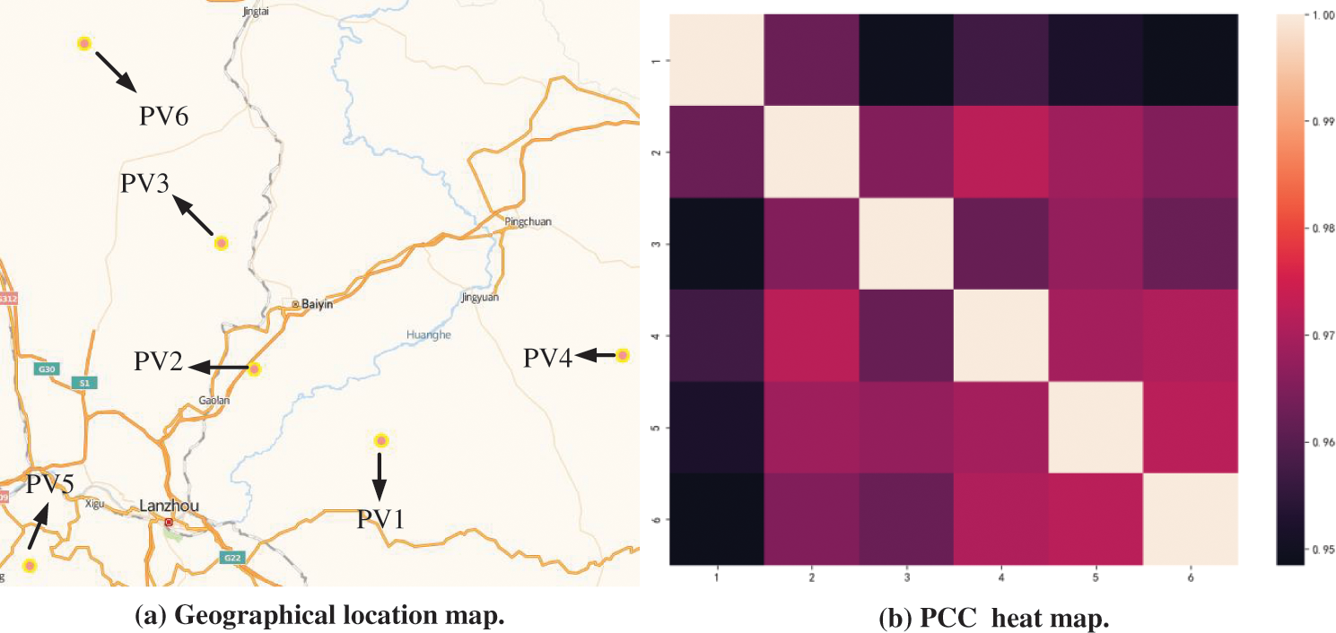
Figure 1: Geographical location and thermal maps of 6 PV power stations

Fig. 1b shows a clear trend in the historical output data from neighboring PV stations, indicating a high correlation. Specifically, the output correlation coefficients show a clear linear relationship with distance over a limited range of distances. This is because the closer the power stations are, the more similar the weather conditions are between them, thus showing similar trends in power generation. It is worth noting that PV stations No. 1 and No. 6 are far apart, resulting in a slight decrease in their correlation coefficient.

Moreover, over a long timescale, the distributed PV output is similar to a periodic single wave of noise. The PV panel surface absorption of irradiance is related to the amount of insolation affected by the daily periodic characteristic of the earth’s rotation. Additionally, weather conditions such as sunny, rainy, and dusty days can all affect the PV panel’s ability to absorb irradiance. This paper further selects representative daily power generation data and irradiance and power generation data under three conditions of clear, rainy, and cloudy skies for each quarter of the year for analysis, as shown in Fig. 2.

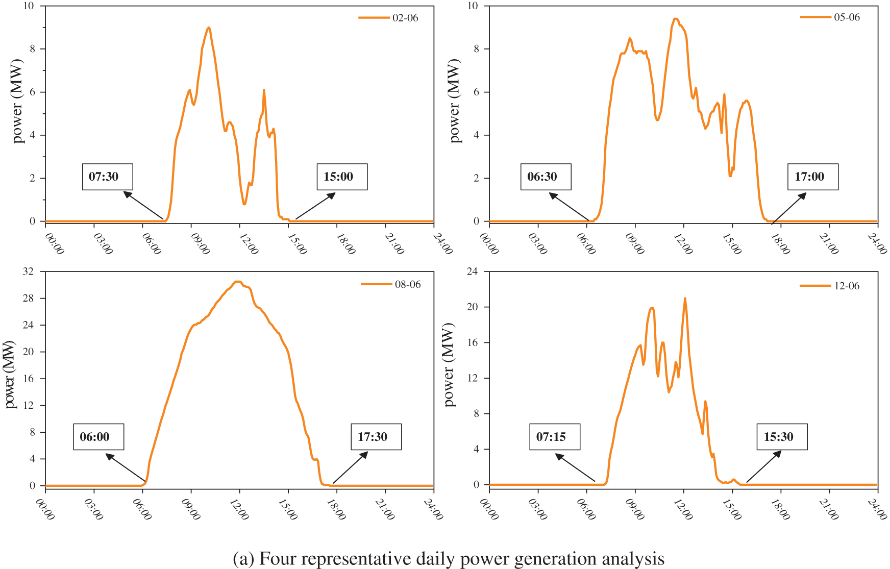
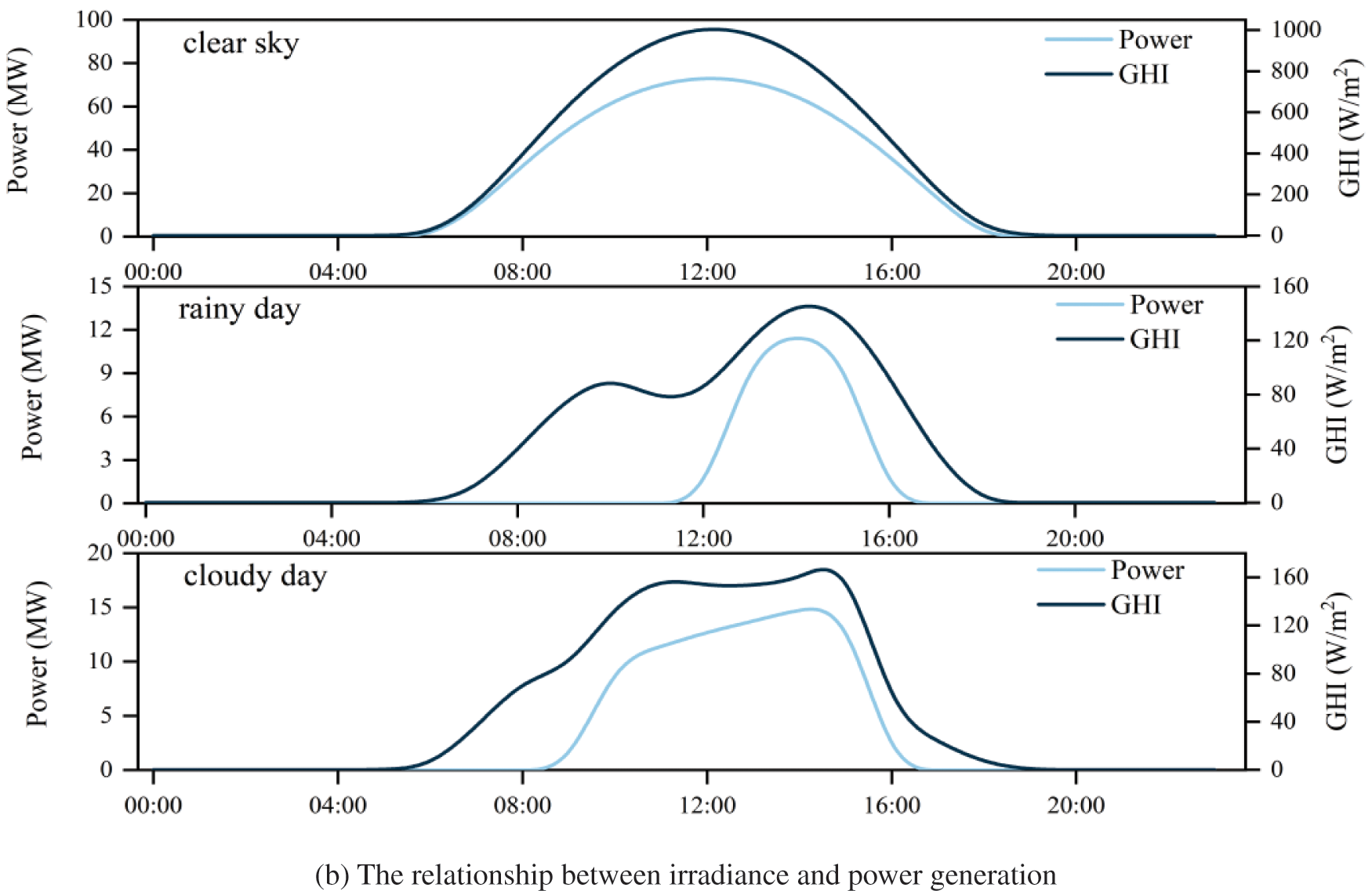
Figure 2: Generation data analysis

Analysis of the power generation data in Fig. 2 shows that PV output has intermittent and stochastic characteristics quickly impacted by weather factors and irradiance. Furthermore, as seen in Fig. 2a for the first and fourth quarters, PV power generation generally starts around 7 a.m. and stops in the afternoon. Power generation in the second and third quarters is comparatively longer. In conclusion, PV’s effective power generation time interval is about 10 h. Further investigation on the relationship between irradiance and power generation for three weather conditions of clear, rainy, and cloudy skies is shown in Fig. 2b. The PV output curve is smoother on sunny days. On the other hand, on rainy and cloudy days, the moving clouds can cause significant fluctuations in the PV station output curve. In addition, the overall output power value of the PV station is lower on overcast days due to the attenuation of solar radiation.

For time series problems requiring continuous data measurements, missing and abnormal data in the data set can interfere with accurate predictions of the forecasting model. Fig. 3 shows abnormal data distribution for the six PV power stations.

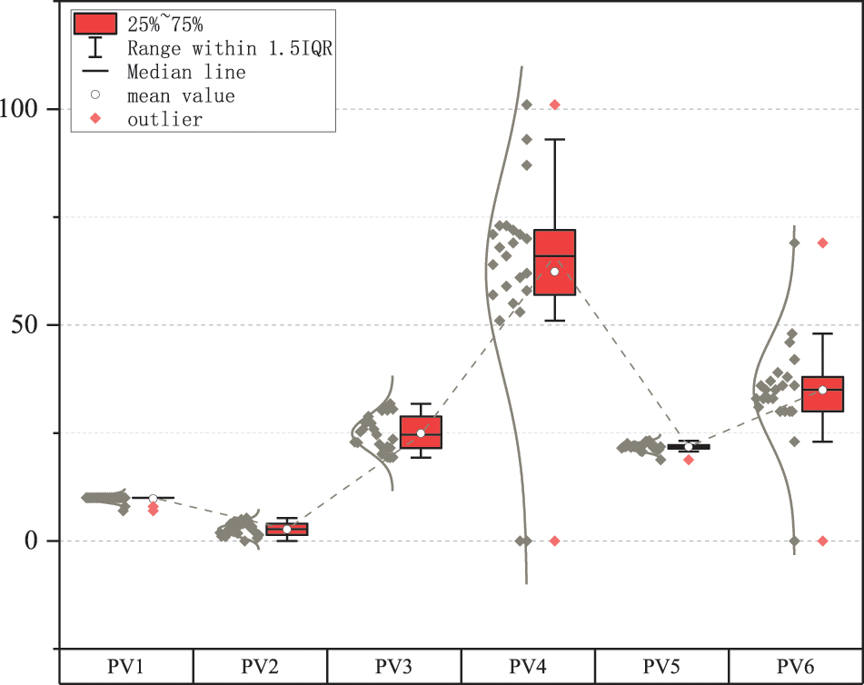
Figure 3: Abnormal data distribution

It is observed that there are many null values (abnormal data) in the data. Furthermore, if the experimental data contains several abnormal data points, it can reduce the experiment’s reliability and lead to false conclusions. Therefore, handling abnormal data is crucial for experiments.

In the case of large samples (e.g., n > 185), the Gaussian distribution rule (3σ rule) [23] is widely used as the crude judgment standard due to its simplicity. Therefore, the 3σ rule is adopted to handle abnormal data in this paper. The specific formula is as follows:

σ=±∑i=1n(xi−x¯)2n−1=±∑i=1n(Δxi)2n−1(1)

Taking PV4 station as an example, the data before and after interpolation according to the 3σ rule is shown in Fig. 4.

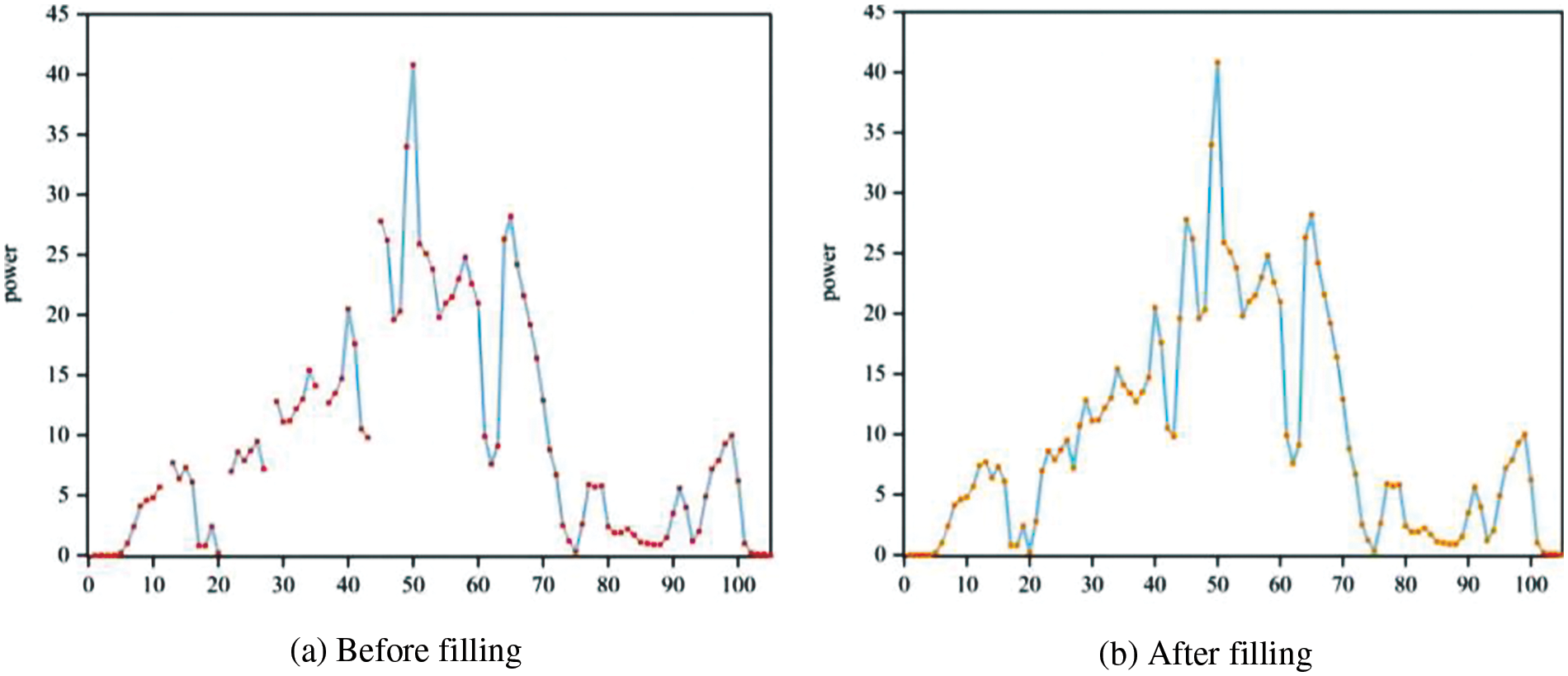
Figure 4: The data filling situation

Therefore, considering factors such as power generation transmission and project development plans, each PV site is processed from a data size of every 5 to every 15 min. The large-scale data of 6 × 105120 is reduced to 6 × 35400, and considering the characteristics of PV power generation, this paper further scales the 6 × 35400 data to 6 × 14600. The first 11680 data sets are used for training, and the last 2920 data sets are used for testing.

Finally, since the unit dimensions of each index differ, normalization and anti-normalization operations are necessary to prevent significant impacts on subsequent calculations and analyses. The formulas are as follows:

x′=x−(xmax−xmin)/2(xmax+xmin)/2(2)

x=(xmax−xmin)x′+(xmax+xmin)2(3)

where xmax and xmin represent the maximum and minimum values in the data.

3  Model

3.1 TCLM Model

This article proposes a Temporal Convolutional-Long Short-Term Memory (TCLM) model for spatio-temporal prediction of distributed PV power stations, which combines the TCN and the LSTM. The TCN captures spatial features among data, whereas the LSTM captures temporal features within the data. The methodology flowchart proposed in this article is shown in Fig. 5.

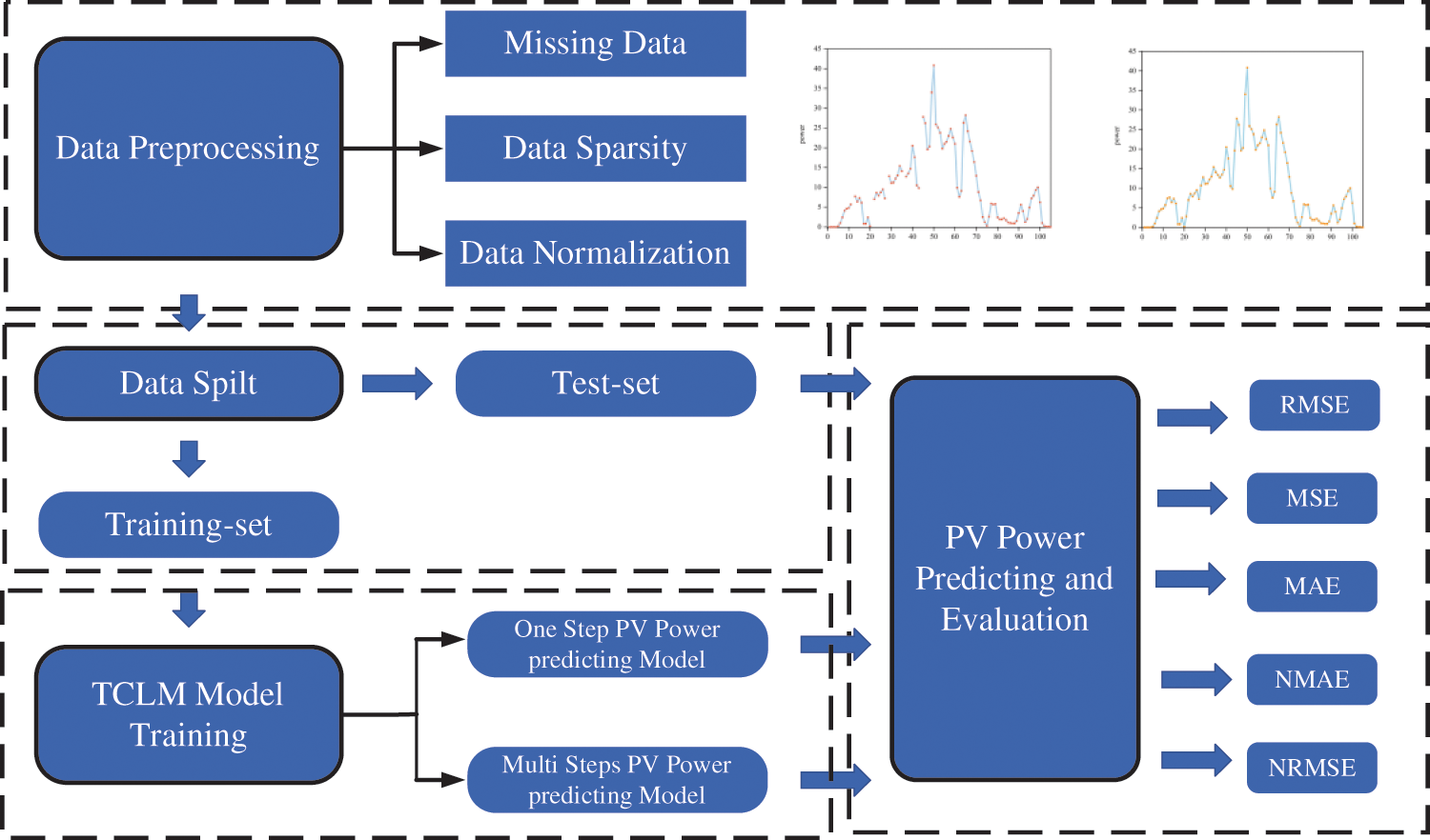
Figure 5: Methodology flowchart

3.2 Temporal Convolutional Networks

The Temporal Convolutional Networks (TCN) is a variation of the convolutional neural network (CNN) [24] that is specifically designed for sequence modeling tasks with causal constraints. The TCN comprises two main components: dilated causal convolution and residual connections.

In Section 3.2, TCN is introduced as a variant of CNN that is specifically utilized for sequence modeling tasks with causal constraints. TCN comprises two essential components: a dilated causal convolution and a residual connection. In the TCN model, the causal convolution ensures the preservation of the temporal order in the input sequence. In contrast, the dilated convolution expands the receptive field to prevent information leakage from the future to the past and minimize computational load. The causality convolution is an efficient way of data processing, which captures the relationship between past inputs and current outputs and can improve processing efficiency by extending the convolution using dilation.

The extended convolution operation F of elements s in a one-dimensional sequence (x∈Rn) for convolution kernel f : {0,1,…,k-1} is expressed as:

F(s)=(x*df)(s)=∑i=1k−1f(i)⋅xs−d⋅i(4)

where d is the dilation factor, i is the number of filters, k is the filter size, and * is the convolution operator. Fig. 6 shows an example of a dilated causal convolution with dilation factors of d = 1, 2, 4 and a filter size of k = 3 to expand the receptive field. To further enlarge the receptive field of the network, larger filter sizes and dilation factors are added.

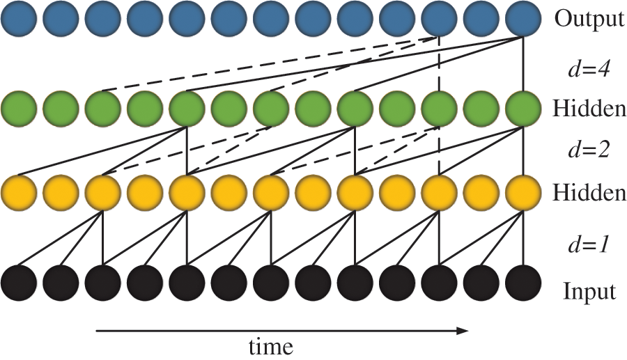
Figure 6: Dilated causal convolution

The TCN communicates information between layers through residual connection modules, which are utilized in a skip-connection manner. Fig. 7 showcases the residual block utilized in this article, which is composed of two layers of dilated causal convolutions and non-linear layers that employ Rectified Linear Units (ReLU) as the activation function. To prevent overfitting, WeightNorm and Dropout layers are implemented after every dilated convolution operation, and an additional 1 × 1 convolution layer is employed to restore the original number of channels.

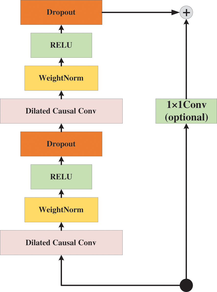
Figure 7: Residual block

3.3 Long Short-Term Memory Networks

Long Short-Term Memory network (LSTM) was first proposed by Hochreiter et al. [19]. Its gating structure can monitor the input, output, and neuron unit state of the data flow in real time to better monitor the transmission of information content. The standard LSTM network structure is shown in Fig. 8, and the detailed principle is shown in Eq. (5).

Figure 8: The unit cell structure of LSTM

it=σ(Wxixt+Whfht−1+bi)ft=σ(Wxfxt+Whfht−1+bf)Ct=ft∘Ct−1+it∘tanh ⁡(Wxcxt+WhcHt−1+bc)ot=σ(Wxoxt+Whoht−1+bo)Ht=ot∘tanh ⁡(Ct)(5)

where Wxi, Whi, Wxf, Whf, Wxc, Whc, and Wxo represent the weight terms, and bf, bi, bc, and bo represent the bias terms. The ° denotes the Hadamard product, xt represents the current input, and ht−1 represents the previous time step’s hidden state. The activation function used in LSTM includes tanh and sigmoid functions.

Compared with the RNN, the significant feature of LSTM is the introduction of the cell state Ct. It not only overcomes the gradient vanishing problem in RNN but also enables the memory of certain information for a long time. Three vectors, including the previous cell state Ct−1, the previous hidden state ht−1, and the current input xt, are inputted to the current unit at each time step. These inputs are outputted to three vectors, ft, it, and ot, respectively, with each vector element between 0 and 1, through each gate. The forget gate determines the relevant historical PV power information and selects them to make better predictions. The input gate decides the final input of current information. The output gate decides which information is used as the final output.

4  Results

4.1 Experiment

All experiments were conducted on Nvidia GeForce RTX 3090Ti with the PyTorch environment in Python3.7. The experiment server is equipped with Intel(R) Xeon(R) Platinum 8358P CPU@2.60 GH and 24 GB memory. In order to prevent the overfitting of neural networks, all models used the early-stopping mechanism with the monitor set as the loss of the validation set. The patience is set as 5.

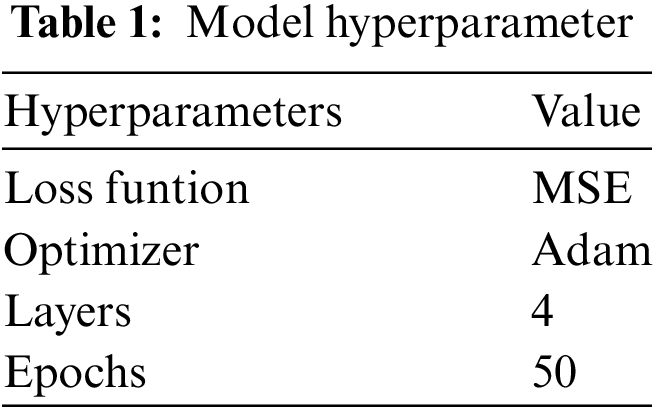
Due to the involvement of a large number of hyperparameters in the models and the significant computational cost involved in each training step, some hyperparameters in this experiment were fixed by experience and summarized in Table 1.

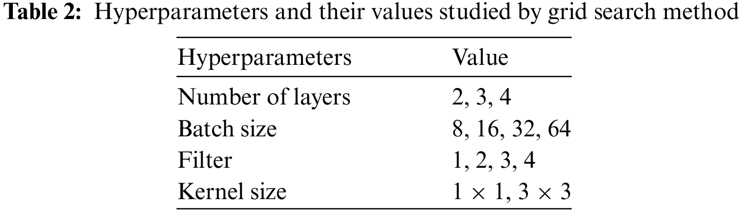
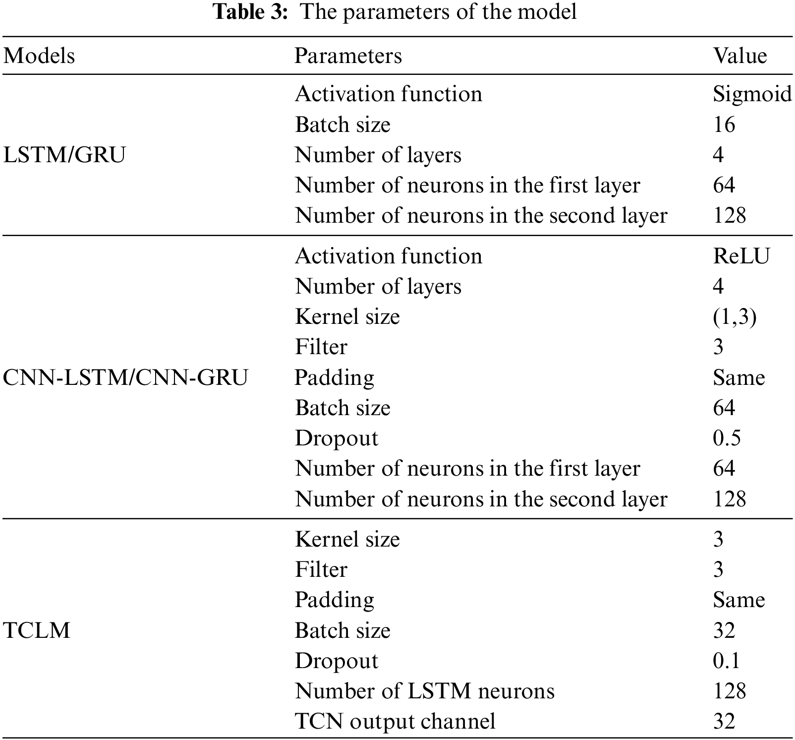
To demonstrate the predictive performance of the proposed TCLM model, it was compared with CNN-LSTM [25], LSTM, Gated Recurrent Unit (GRU) [26] and CNN-GRU [27]. Since the remaining parameters are always considered to be the main contributors to the network performance, a grid search approach is used to determine the optimal model settings by examining their possible combinations. The hyperparameters to be tuned include batch size, Number of Layers, filter, and kernel size, whose values are specified in Table 2. After grid search, all model hyperparameters are shown in Table 3.

To evaluate the accuracy of the model in predicting the results and measure the discrepancy between the predicted and actual results, five evaluation indicators were utilized. These include Mean Absolute Error (MAE), Mean Square Error (MSE), Root Mean Squared Error (RMSE), Normalized Mean Absolute Error (NMAE), and Normalized Root Mean Squared Error (NRMSE). These indicators are presented as follows:

MAE=1m∑i=1m|yi−y^i|(6)

MSE=1m∑i=1m(yi−y^i)2(7)

RMSE=1m∑i=1m(yi−y^i)2(8)

NRMSE=1m∑i=1m(yi−y^i)2(ymax−ymin)2(9)

NMAE=1m∑i=1m|yi−y^i|(ymax−ymin)(10)

where yi represents the real PV power data, yi∧ represents the predicted value, m represents the number of test sets, ymax, and ymin represent the maximum and minimum values of PV power in the test set.

RMSE, MAE, and MSE are used to evaluate the performance of the regression model. The lower the value, the higher the predictive accuracy. NRMSE and NMAE are obtained by normalizing RMSE and MAE, respectively, and the lower the NRMSE and NMAE values indicate the more stable predictive performance and higher predictive accuracy of the model.

4.2 Single-Step Prediction Performance

TCLM, LSTM, GRU, CNN-GRU and CNN-LSTM were compared in terms of single-step prediction of the output power of each PV station, with the input of 3D tensor (14595, 5, 6), and the last step (15 min) was predicted based on the first four steps (1 h).

Firstly, this paper compared the single-step predictions of the four models for the output power of each PV station, and Table 4 describes the prediction errors of the four models.

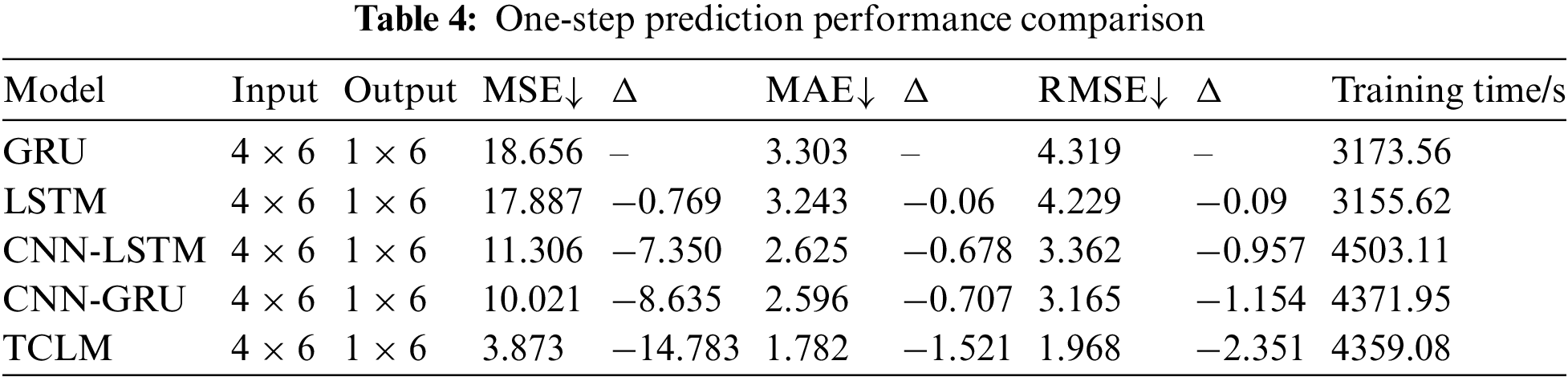
As presented in Table 4, the GRU model exhibits the lowest predictive accuracy, yielding MSE, MAE, and RMSE values of 18.656, 3.303, and 4.319, respectively. Although LSTM demonstrates a slightly enhanced predictive accuracy compared to GRU, the improvement is not statistically significant. This observation underscores the proficient performance of both LSTM and GRU in handling time series data, albeit with suboptimal results when applied to the prediction of cluster-distributed PV power stations, considering their spatial dimension. In contrast, the CNN-LSTM model, which combines CNN for spatial feature extraction and LSTM for temporal feature extraction, notably enhances predictive accuracy. This suggests that the integration of CNN and LSTM surpasses the standalone LSTM and GRU models in predictive performance. Further comparison of CNN-LSTM and CNN-GRU models reveals that CNN-GRU has slightly improved prediction accuracy. Furthermore, compared to the CNN-GRU model, the TCLM model introduced in this paper achieves the highest prediction accuracy, boasting MSE, MAE, and RMSE values of 3.873, 1.782, and 1.968, respectively.

Regarding prediction training time, the prediction models using LSTM and GRU networks have short training times, but LSTM and GRU networks have the lowest prediction accuracy. Similar to the prediction accuracy performance, the prediction time of CNN-LSTM and CNN-GRU networks is also similar. Further, the model proposed in this paper significantly improves the prediction accuracy, although the prediction time is improved by 12.87 s compared to CNN-GRU. This indicates that using TCLM can reduce the training and prediction time of the system while maintaining prediction accuracy.

To further validate the single-step prediction performance of the proposed model, this paper presents a comparison of the NMAE and NRMSE errors of four models, as shown in Fig. 9.

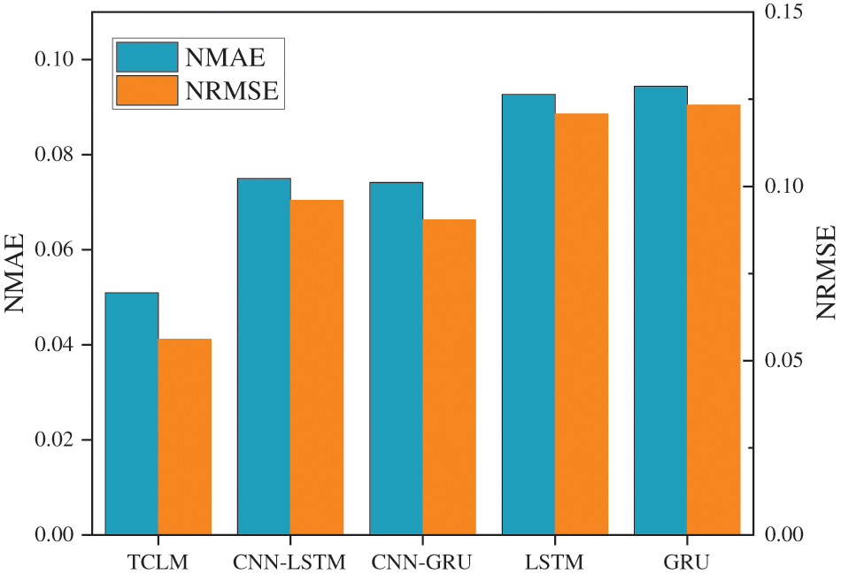
Figure 9: The comparison of single-step prediction errors

It can be observed from Fig. 9 that the CNN-LSTM model exhibits superior prediction accuracy compared to the baseline LSTM and GRU models, achieving NMAE and NRMSE values of 0.075 and 0.096, respectively. Further comparison of CNN-LSTM and CNN-GRU models reveals that CNN-GRU has slightly improved prediction accuracy. This is because CNN-GRU has fewer parameters relative to CNN-LSTM. This means that the CNN-GRU model may require less data and computational resources to achieve similar predictive performance during training. Moreover, the TCLM model demonstrates significantly enhanced prediction accuracy in comparison to the CNN-GRU model, yielding NMAE and NRMSE values of 0.0509 and 0.056, respectively. These findings indicate that the proposed TCLM spatio-temporal prediction model offers high accuracy in predicting distributed PV spatio-temporal patterns and proves to be effective in this regard.

4.3 Multi-Step Prediction Performance

The last section of this paper discusses the exceptional performance of the proposed TCLM model in single-step prediction. To further validate the predictive capabilities of the proposed model, this section proceeds to conduct multi-step prediction built upon single-step prediction. The input step length of all models is fixed at 4 (1 h), but the output step length is changed to 2 (30 min), 3 (45 min), and 4 (1 h). The comparison results of output power prediction accuracy for different output step lengths are shown in Table 5.

Table 5 reveals that, with an increase in the prediction step length, all models exhibit a noticeable decline in prediction accuracy. Both LSTM and GRU models effectively leverage historical output power data from all PV power stations within the designated region. In contrast, the CNN-LSTM and CNN-GRU models outperform the benchmark LSTM model and GRU model in both single-step prediction and multi-step prediction, highlighting the advantages of these two hybrid models in predicting long-time series. Further analysis shows that CNN-GRU outperforms CNN-LSTM in 2-step, 3-step, and 4-step prediction. The model introduced in this study, TCLM, combines a TCN with LSTM, and it achieves the highest accuracy in multi-step prediction. The average MAE, MSE, and RMSE are 3.33, 14.01, and 2.72, respectively.

Further validation of the proposed model shows the NRMSE and NMAE error plots of four methods, as shown in Fig. 10.

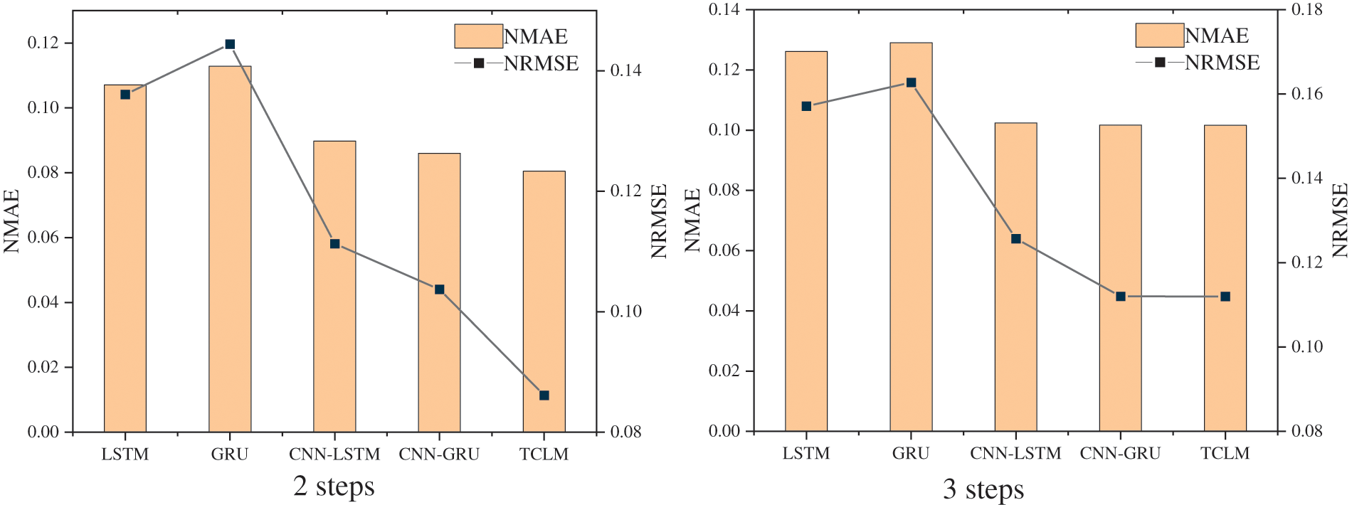
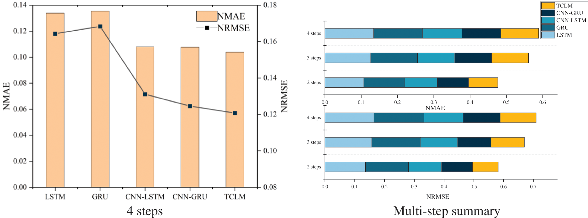
Figure 10: NMAE, NRMSE comparison for different steps

Fig. 10 shows that the prediction accuracies of all models decrease as the prediction step increases. The NMAE and NRMSE of the TCLM model are lower than those of the other four models. In addition, the prediction accuracy of the TCLM model, which combines a temporal convolutional neural network and a long and short-term memory network, is better than that of the CNN-LSTM and CNN-GRU models at different output steps, and its average NMAE and NRMSE are 0.095 and 0.106, respectively. In the case of multi-step outputs, the proposed TCLM model can accurately consider the temporal characteristics of the output power and the spatial characteristics of the input data and provide accurate modeling analysis and prediction of the spatio-temporal data.

5  Conclusion

This research introduces a spatio-temporal prediction model termed the Temporal Convolutional-Long Short-Term Memory (TCLM) model, which amalgamates the temporal convolutional network with the long short-term memory network. To assess the model’s effectiveness, we conducted validation using a dataset comprising 14,600 instances sourced from a specific region in Gansu Province, China. Through meticulous case analysis and verification, the following key findings have been established:

1.    Missing and anomalous data from data transmission and storage have been meticulously addressed using the 3σ criterion. Moreover, the data dimensionality has been reduced by incorporating insights from the spatio-temporal distribution pattern of photovoltaic (PV) output.

2.    Our study introduces a hybrid model that synergizes the temporal convolutional network with the long short-term memory network. This innovative approach facilitates spatial information extraction via the TCN component and captures temporal features through LSTM.

3.    The proposed model in this study has demonstrated exceptional predictive performance across both one-step and multi-step prediction scenarios when benchmarked against three alternative models. Notably, it has achieved an average Normalized Root Mean Square Error (NRMSE) of 0.0842. Multi-step average Mean Absolute Error (MAE) and Root Mean Squared Error (RMSE) are 3.33 and 3.72, respectively.

This investigation has been centered on the spatio-temporal prediction of distributed PV power generation, encompassing diverse scenarios. It presents a novel avenue for optimizing the coordination of distributed PV and energy storage systems. Nevertheless, there remains scope for enhancing the predictive accuracy of the model. Future endeavors will explore various strategies to augment the model’s performance, including: (1) Integration of additional external information, such as satellite imagery, to adapt to longer prediction horizons, spanning 12 to 36 h. (2) Emphasis on developing robust predictive models with inherent resistance to data contamination from transmission issues.

Acknowledgement: None.

Funding Statement: The Science and Technology Project of the State Grid Corporation of China (Research and Demonstration of Loss Reduction Technology Based on Reactive Power Potential Exploration and Excitation of Distributed Photovoltaic-Energy Storage Converters: 5400-202333241A-1-1-ZN).

Author Contributions: The authors confirm contribution to the paper as follows: study conception and design: K. Liu, C. Liang; data collection: X. Dong; analysis and interpretation of results: L. Liu; draft manuscript preparation: C. Liang, X. Dong. All authors reviewed the results and approved the final version of the manuscript.

Availability of Data and Materials: Data will be made available on request.

Conflicts of Interest: The authors declare that they have no conflicts of interest to report regarding the present study.

References

1. Wang, J., Hu, Z., Xie, S. (2019). Expansion planning model of multi-energy system with the integration of active distribution network. Applied Energy, 253, 113517. [Google Scholar]

2. Kushwaha, P., Prakash, V., Bhakar, R., Yaragatti, U. R. (2022). Synthetic inertia and frequency support assessment from renewable plants in low carbon grids. Electric Power Systems Research, 209, 107977. [Google Scholar]

3. Wang, Y., Wang, Y., Huang, Y., Yang, J., Ma, Y. et al. (2019). Operation optimization of regional integrated energy system based on the modeling of electricity-thermal-natural gas network. Applied Energy, 251, 113410. [Google Scholar]

4. Gilasi, Y., Hosseini, S. H., Ranjbar, H. (2022). Resiliency-oriented optimal siting and sizing of distributed energy resources in distribution systems. Electric Power Systems Research, 208, 107875. [Google Scholar]

5. Gao, Y., Ai, Q., He, X., Fan, S. (2023). Coordination for regional integrated energy system through target cascade optimization. Energy, 276, 127606. [Google Scholar]

6. Fonseca Junior, J. G. D. S., Oozeki, T., Ohtake, H., Takashima, T., Ogimoto, K. (2015). Regional forecasts of photovoltaic power generation according to different data availability scenarios: A study of four methods. Progress in Photovoltaics: Research and Applications, 23(10), 1203–1218. [Google Scholar]

7. Saint-Drenan, Y. M., Good, G. H., Braun, M. (2017). A probabilistic approach to the estimation of regional photovoltaic power production. Solar Energy, 147, 257–276. [Google Scholar]

8. Pierro, M., de Felice, M., Maggioni, E., Moser, D., Perotto, A. et al. (2017). Data-driven upscaling methods for regional photovoltaic power estimation and forecast using satellite and numerical weather prediction data. Solar Energy, 158, 1026–1038. [Google Scholar]

9. Visser, L., AlSkaif, T., van Sark, W. (2022). Operational day-ahead solar power forecasting for aggregated PV systems with a varying spatial distribution. Renewable Energy, 183, 267–282. [Google Scholar]

10. Zang, H., Liu, L., Sun, L., Cheng, L., Wei, Z. et al. (2020). Short-term global horizontal irradiance forecasting based on a hybrid CNN-LSTM model with spatiotemporal correlations. Renewable Energy, 160, 26–41. [Google Scholar]

11. Wang, F., Lu, X., Mei, S., Su, Y., Zhao, Z. et al. (2022). A satellite image data based ultra-short-term solar PV power forecasting method considering cloud information from neighboring plant. Energy, 238, 121946. [Google Scholar]

12. Yang, X., Yang, Y., Meng, L., Zhao, Y. (2023). Spatio-temporal PV power forecasting considering the time-shift correction and the information fusion strategy of multi-stations. ISA Transactions, 139, 376–390. [Google Scholar] [PubMed]

13. Wang, J., Huang, Y., Li, C., Xiang, K., Lin, Y. et al. (2020). Time series modeling method for multi-photovoltaic power stations considering spatial correlation and weather type classification. Power System Technology, 44(4), 1376–1384. [Google Scholar]

14. Yan, J., Mu, L., Wang, L., Ranjan, R., Zomaya, A. Y. (2020). Temporal convolutional networks for the advance prediction of ENSO. Scientific Reports, 10(1), 8055. [Google Scholar] [PubMed]

15. Gao, H., Jia, H., Yang, L. (2022). An improved CEEMDAN-FE-TCN model for highway traffic flow prediction. Journal of Advanced Transportation, 2022, 1–20. [Google Scholar]

16. Wang, C., Zhang, W., Wu, C., Hu, H., Zhu, W. (2022). Combined prediction method of short-term distance headway based on EB-GRA-TCN. Journal of Advanced Transportation, 2022, 1–12. [Google Scholar]

17. Liu, S., Ning, D., Ma, J. (2023). TCNformer model for photovoltaic power prediction. Applied Sciences, 13(4), 2593. [Google Scholar]

18. Li, Y., Song, L., Zhang, S., Kraus, L., Adcox, T. et al. (2023). A TCN-based hybrid forecasting framework for hours-ahead utility-scale PV forecasting. IEEE Transactions on Smart Grid, 14(5), 4073–4085. [Google Scholar]

19. Hochreiter, S., Schmidhuber, J. (1997). Long short-term memory. Neural Computation, 9(8), 1735–1780. [Google Scholar] [PubMed]

20. Li, K., Huang, W., Hu, G., Li, J. (2023). Ultra-short term power load forecasting based on CEEMDAN-SE and LSTM neural network. Energy and Buildings, 279, 112666. [Google Scholar]

21. Cho, K., Kim, Y. (2022). Improving streamflow prediction in the WRF-Hydro model with LSTM networks. Journal of Hydrology, 605, 127297. [Google Scholar]

22. Li, G., Zhang, A., Zhang, Q., Wu, D., Zhan, C. (2022). Pearson correlation coefficient-based performance enhancement of broad learning system for stock price prediction. IEEE Transactions on Circuits and Systems, 69(5), 2413–2417. [Google Scholar]

23. Xia, J., Zhang, J., Wang, Y., Han, L., Yan, H. (2022). WC-KNNG-PC: Watershed clustering based on k-nearest-neighbor graph and Pauta Criterion. Pattern Recognition, 121, 108177. [Google Scholar]

24. Krizhevsky, A., Sutskever, I., Hinton, G. E. (2012). Imagenet classification with deep convolutional neural networks. Advances in Neural Information Processing Systems, 25, 1–9. [Google Scholar]

25. Vidal, A., Kristjanpoller, W. (2020). Gold volatility prediction using a CNN-LSTM approach. Expert Systems with Applications, 157, 113481. [Google Scholar]

26. Li, C., Tang, G., Xue, X., Saeed, A., Hu, X. (2019). Short-term wind speed interval prediction based on ensemble GRU model. IEEE Transactions on Sustainable Energy, 11(3), 1370–1380. [Google Scholar]

27. Zhao, Z., Yun, S., Jia, L., Guo, J., Meng, Y. et al. (2023). Hybrid VMD-CNN-GRU-based model for short-term forecasting of wind power considering spatio-temporal features. Engineering Applications of Artificial Intelligence, 121, 105982. [Google Scholar]