Rolling Decision Model of Thermal Power Retrofit and Generation Expansion Planning Considering Carbon Emissions and Power Balance Risk

1  Introduction

To mitigate the global environmental problems caused by climate change, in September 2020, China proposed the “3060 Dual Carbon Target” at the United Nations General Assembly. The electric power industry plays a key role in China’s energy-saving and emission-reduction strategy. Statistics show that coal and other fossil energy power stations account for 47% of the CO2 emissions in China [1]. To achieve the “dual carbon target”, it is imperative to plan low-carbon power supplies on the power side.

Currently, extensive research has been conducted on low-carbon power planning domestically and internationally. Various power planning methods exist, including but not limited to multi-objective robust, two-layer programming, multi-stage programming, and other modeling methods [2–4]. Low-carbon power supply planning research is mainly divided into two directions: indirect achievement through the introduction of environmental protection policies and carbon trading systems [5], and direct achievement through the introduction of emission reduction technology and clean energy. Zhang et al. [6] incorporated the green certificate trading mechanism and carbon trading mechanism into the power supply planning model, aiming to maximize the system’s net income during the planning period. Wang et al. [7] introduced wind farms and CO2 emission environmental cost into the power supply planning model, utilized multi-scenario modeling to finely divide the system operation, and applied an improved genetic algorithm for model optimization.

Carbon dioxide capture and storage are technologies introduced in low-carbon power generation to mitigate the environmental impact of power plants [8]. Carbon Capture and Storage (CCS) technology has a significant impact on carbon emission reduction of thermal power units. Carbon capture equipment consumes a portion of the unit's output to recover CO2 from the flue gas, achieving carbon reduction in thermal power units. Emission and output loss models of CCS power plants were constructed by Lu et al. [9] and Chen et al. [10]. Zhong et al. [2] planned new wind farms, thermal power units, CCS units, and existing thermal carbon capture retrofit with a multi-objective robust optimization method. Considering the requirements of operation safety and economy comprehensively, a power supply planning model for power plants with CCS was established by Ji et al. [11].

Concurrently, driven by the “dual carbon target,” renewable energy power generation has rapidly developed, significantly improving its cost efficiency and competitiveness [12]. The large-scale connection of renewable energy to the grid can promote carbon emission reduction [13]. Huang et al. [14] selected representative scenarios based on demand and wind power output duration curves, considering the correlation of demand and wind power output, and utilized the stochastic optimization (SO) method to develop a generation and transmission expansion planning model that takes into account low-carbon factors. Abaul et al. [15] developed a framework to address the emission-constrained generation expansion problem using the GAMS optimization tool, aiming to minimize carbon emissions and costs. Zhou et al. [16] proposed a coordinated expansion planning model for the sending power network based on HVDC and hydro-solar coordination and complementarity. However, the volatility of its output increases the operational risk of the system. Shang et al. [17] proposed a risk assessment model for power system operation considering wind and PV grid connection and established a comprehensive risk assessment index by combining the Analytic Hierarchy Process (AHP) and Entropy Weight Method (EWM). Zhang et al. [18] used a conditional value-at-risk quantification system to quantify system scheduling operation risk and proposed a two-stage optimal scheduling model that takes operational risk and standby availability into account. However, the above studies failed to quantitatively assess the system emission reduction and operational risks after low-carbon planning, resulting in problems such as excessive carbon emissions and frequent load cutting on some days while meeting the annual carbon reduction standards.

Given the issues such as excessive carbon emissions, inadequate consumption of renewable energy, and load shedding during intra-day power system operations, and considering the characteristics of power regulation and the fluctuating nature of renewable energy, this paper proposes risk assessment indicators and methods for carbon emissions and power balance. Secondly, based on the traditional two-layer power planning model (investment tier and operation tier), a lower risk assessment tier decision model is established to consider carbon emission and power balance risk. The model is simplified into a two-tier rolling decision model, incorporating the investment decision tier and the simulation operation and risk assessment tier, which considers the risk of carbon emission and power balance, and makes decisions on the scale of thermal power unit retrofit and new units annually, through the coupling relationship between the three tiers. The decision method described in this paper can reduce the number of high-risk days and the magnitude of carbon emissions during power system operation, thereby reducing the power balance risk.

2  Carbon Emission and Power Balance Risk Assessment Method

This paper proposes a combined system front-day unit combination model, along with carbon emission and power balance risk assessment indicators and assessment methods, to quantify the risks arising from the uncertainty of renewable energy output. Additionally, it establishes an uncertainty scenario set for renewable energy output at each time. Through stochastic production simulation of these uncertain scenarios, the paper achieves a quantitative assessment of carbon emission risk and power balance risk.

2.1 Renewable Energy Timing Uncertainty Scenario Construction Method

In this paper, the timing uncertainty scenario of renewable energy is established by considering the randomness and timing of the landscape forces. This is achieved through the use of a probability distribution model and a time series model, which together form the renewable energy timing uncertainty scenario.

Wind power output varies with wind speed. Weibull distribution is usually used to express wind speed fluctuation. The probability density function of wind speed fluctuation [19]:

f(v)=kc(vc)k−1exp⁡[−(vc)k](1)

where, v is wind speed, and only between the cut in wind speed vin and cut out vout wind speed, the wind turbine can be normal output; k is the shape parameter; c is the scale parameter.

Because of the seasonal and diurnal characteristics of wind speed, the wind speed at the same time of the same month and day of the year can be expressed in the same probability distribution. The wind power timing uncertainty scenario is generated as follows: First, to simplify the calculation, an equal number of typical days are extracted from each month or week. Secondly, the vin and vout intervals of wind turbines are divided into s sub-intervals, and the midpoint of the sub-intervals is the s-th timing scenario wind speed vt,s, and each wind speed corresponds to the wind power output at the current moment. The wind power conversion relationship can be approximated as satisfying the following relationship [20]:

Pt,sWpl={0,vt,s>vout,vt,s≤vina+bvt,s,vin<vt,s<vNPNW,vN<vt,s<vout(2)

where, Pt,sWpl is wind power timing scenario forecast generation; vN is rated wind speed; PNW is rated output power of the fan; a and b can be calculated according to the continuity of Pt,sWpl and are both constants.

Finally, according to different k and c parameters at different times, the uncertainty scenario probability of wind power fluctuation with wind speed fW(vt,s) is obtained from Eq. (1). Similarly, the scene output and probability of the photovoltaic (PV) output uncertainty scenario can also be obtained from the above steps. The PV output is proportional to the light intensity r. The r adopts Beta distribution [21]. The probability density function of r is:

f(r)=Γ(y+z)Γ(y)Γ(z)(rrmax)y−1(1−rrmax)z−1(3)

where, y and z are the shape parameter of Beta distribution; rmax is the maximum light intensity in the area; Γ is Gamma function.

The forecast generation of the PV timing scenario is obtained by Eq. (4):

Pt,sPVpl=rt,sAη(4)

where, rt,s is timing scene light intensity, the corresponding timing scenario probability is fPV(rt,s); A is the effective area of the PV cell array; η is PV conversion rate of PV cell array.

2.2 Carbon Emission Risk Index of Power System

The term “carbon emission risk” generally refers to the risk of excessive system carbon emissions [22] or the environmental risk resulting from carbon emissions under uncertain factors such as renewable energy fluctuations. In this paper, carbon emission risk is specifically defined as the economic and environmental security risk arising from the anticipated carbon emissions of thermal power units exceeding the daily carbon emission limit due to the uncertainty of renewable energy. The output and carbon emission of thermal power units before and after carbon capture retrofit (unit, ton) are calculated as follows:

Enc(Pi,ts)=αiPi,ts(5)

Eyc(Pi,ts)=(1−β)Enc(Pi,ts)(6)

where, Enc and Eyc are carbon emissions from thermal power without retrofit and after retrofit, respectively; Pi,ts is the output of the i-th thermal power unit under the s-th scenario at time t; αi is the carbon emission coefficient of thermal power units; β is the capture rate of carbon capture equipment.

According to the above definition, carbon emission risk indicators are as follows:

RE={Ed−E0d Ed≥E0d0Ed<E0d(7)

where, RE is the daily carbon emission risk level, 0–5 is low risk, 5–10 is medium risk, and >10 is high risk; E0d is the daily safe carbon emission threshold, which is assigned by the annual carbon emission quota weighted by the annual proportion of the daily load; Ed is the expected carbon emissions for the day:

Ed=∑t=1T∑sft(s)[∑i∈ΘycEyc(Pi,ts)+∑i∈ΘncEnc(Pi,ts)](8)

where, T takes 24 h; Θyc and Θnc are the thermal power collection with and without retrofit, respectively. ft(s) is timing scenario probability, which is ft(s)=fW(vt,s)fPV(rt,s).

2.3 Power Balance Risk Index of Power System

The abandonment of wind and solar energy sources or load shedding can impact the economy and reliability of the power system [23], leading to power imbalance. In the optimization operation process, the expected value and expression of the two, PB and LB, are as follows:

PB=∑t=1T∑sft(s)[(Pt,sWpl−Pw,ts)+(Pt.sPVpl−Pp,ts)](9)

LB=∑t=1T∑sft(s)(Lt−Ltact,s)(10)

where, Pw,ts and Pp,ts are the on-grid power of solar power in the s-th scene at time t; Ltact,s is the actual load supply under the s-th system timing scenario; Lt is the system load at time t.

Considering the power regulation characteristics of energy storage and the uncertainty of renewable energy, the power balance risk including both is established in this paper. The risk index value is obtained by summing PB and LB with a certain weight to describe the risk level:

RB=ϖ1PB+ϖ2LB(11)

where, ϖ1 and ϖ2 are the weights of the above risk indicators, respectively; RB is the daily power balance risk level, ‘0–1’ is low risk, ‘1–3’ is medium risk, and ‘>3’ is high risk.

The different weights of the index k obtained by EWM and AHP are summarized, ϖE,k and ϖA,k. The comprehensive weight of indicators is determined by Eq. (12):

ϖk=ϖE,kϖA,k∑k=12ϖE,kϖA,k(12)

2.4 Risk Assessment Method

In this paper, combined with the unit combination model, the state of thermal power start-stop vi,t, charging and discharging state of energy storage ut and timing capacity of energy storage ESt corresponding to the prediction curve are determined. Then, the sequential production simulation is carried out for different scenarios s, and the production and load absorption under the timing scenario of the power system are obtained. Then, the daily risk index is calculated according to Eqs. (5)–(11) to evaluate the risk level of carbon emission and power balance. The evaluation methods and procedures are as follows:

Step 1: Unit combination: According to the renewable energy and load predicted value to determine the power supply within the day of the shutdown state;

Step 2: According to the probability and statistical characteristics of renewable energy output fluctuation, the timing uncertainty scenario set of renewable energy output is generated ΘS;

Step 3: According to the starting state of the unit, the unit is re-combined, and the output and load absorption of the unit in each scenario is calculated;

Step 4: Calculate the daily risk indicators of carbon emission and power balance according to the probability ft(s) and Eqs. (5)–(11) of scenario s, and evaluate the risk degree according to the size of the risk indicators.

The assessment methods and processes are shown in Fig. 1.

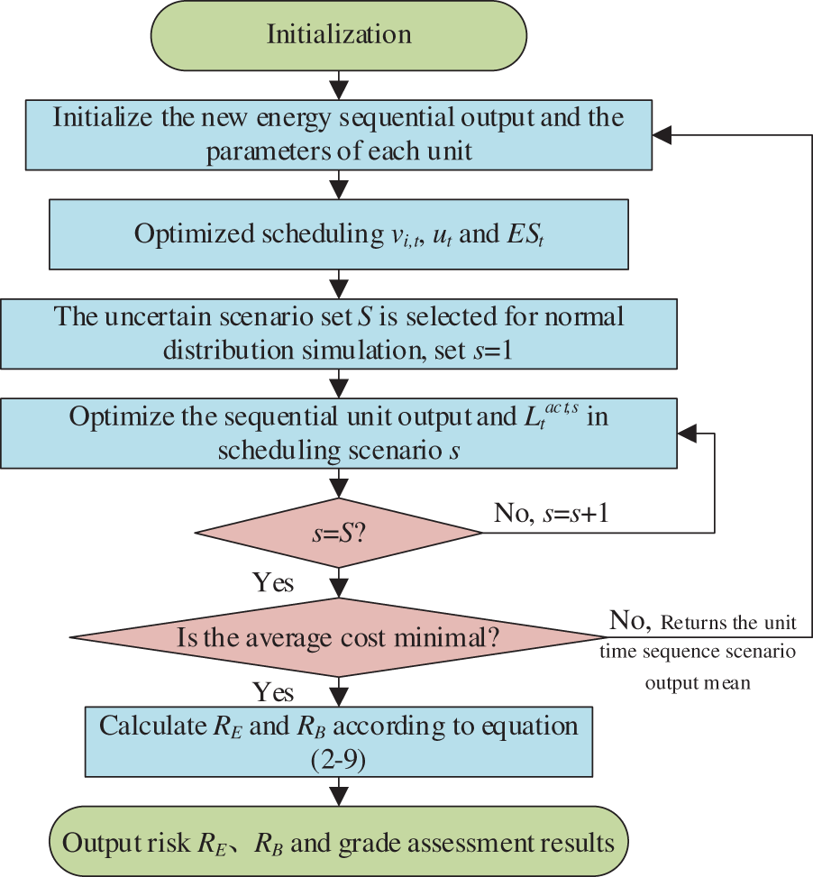
Figure 1: Assessment methods and processes

3  Rolling Decision Model Considering Carbon Emission and Power Balance Risk

In this paper, a rolling decision model for thermal power retrofit and generation expansion planning is established, taking into account the annual growth rate of investment and operating costs. This model enables decisions to be made on the number of thermal power unit retrofits, as well as the type and capacity of units in operation on a rolling year-by-year basis. The model consists of three tiers: investment decision, operation simulation, and risk assessment. To assess carbon emission risk and power balance risk, an assessment model tier is added to the proposed rolling planning model based on the results of the lower-level operational model. The investment decision model determines the projects for thermal unit construction and retrofit. In line with the upper-tier decision scheme, the operation simulation tier model obtains typical daily load values, renewable energy output forecast values, thermal power start-stop, energy storage charge and discharge, and time series capacity state. Based on the results of stochastic production simulations and uncertain scenarios from the mid-tier, the risk assessment tier model assesses carbon emission and power balance risk in decision-making.

3.1 Model Framework and Objective Function

For traditional generation expansion planning of power systems, the renewable energy timing uncertainty is generally not considered at the operational level. The risk assessment proposed in this paper is based on the consideration of renewable energy time-series uncertainty, which results in a proliferation of decision variables. Therefore, a new tier of risk assessment is added as the lowest layer based on the traditional investment tier and operation tier of two-tier unit planning in this paper. Considering carbon emission and power balance risk, the minimum sum of timing scenario operation and risk assessment weighted values are the lower tier objectives. The objective function of the decision model is shown in Eq. (13):

minobj=ϖnCn+ϖopCop+ϖrCr(13)

where, Cn is annual investment cost; Cop is the daily operating cost sum of forecast output; ϖn, ϖop and ϖr are cost factors for each objective, respectively, which are determined manually according to the decision center of gravity.

The objective components of each layer can be expressed as follows:

Cn=min(CNT+CNW+CNPV+CNS+CETC+CNTC)(14)

Cop=min∑d(CYC+CNC+CDU+Cs)(15)

Cr=min(ϖC1s∑s,tCopt,s+ϖRRop)(16)

where, CNT, CNW, CNPV and CNS are investment costs of new thermal power units, wind power units, PV units, and energy storage equipment, respectively; CETC and CNTC are investment cost of retrofit of the original and new thermal power units, respectively; CYC, CNC, CDU and Cs are predicted operating costs of retrofit and non-retrofit thermal power units, start-up and shutdown costs of thermal power units and predicted operating costs of energy storage, respectively; Copt,s is the operation cost for timing scenarios; Rop is the comprehensive risk index value; ϖC and ϖR are the objective coefficient of Copt,s and Rop, respectively.

According to the traditional two-tier planning model and the risk assessment method proposed in this paper, a coupling relationship between the three-tier model is illustrated in Fig. 2. The upper investment tier conveys the decision result regarding the construction state of all units to be built and the retrofit state of all thermal power units to the middle operating tier. Economic optimization of unit combination is then conducted, followed by operation simulation [24], and the outcomes of unit start-stop and energy storage charging and discharging states are transferred to the lower evaluation tier. Through the combination of economic and risk-value optimization of sequential units for each scenario, production simulation of timing scenarios is executed. The final middle-tier forecast operation cost and lower-tier scenario operation average cost are returned to the three-tier total objective to minimize the total cost. This demonstrates a close coupling relationship between the prediction operation tier and the risk assessment tier, as both involve production simulation and share some decision variables and constraints. To simplify and facilitate model solving, the predicted value is treated as one of the scenarios, and the start-stop and charge-discharge state of units is determined by the mean of the scenario output. The two-tier planning framework with the middle and lower tiers combined into one tier is shown in Fig. 3. The objective of the new two-tier model is:

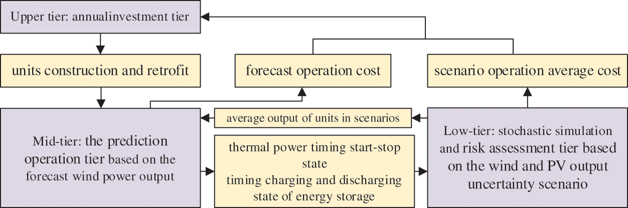
Figure 2: Coupling relationship between multi-level models

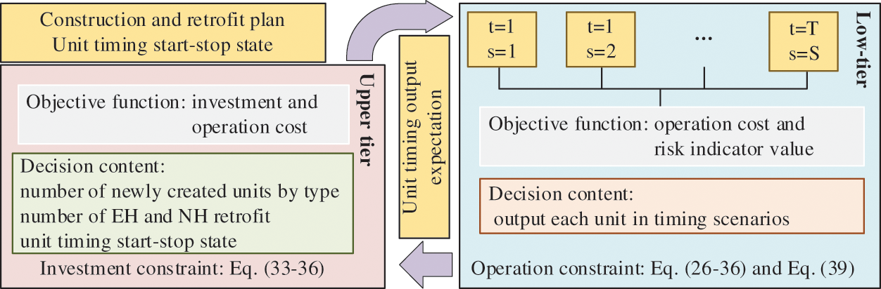
Figure 3: Framework of two-layer planning model

minobj=ϖnCn+ϖlCl(17)

where, ϖl and Cl are the cost factor and objective of the simplified new low-tier, operational, and risk assessment tier, respectively.

3.2 Investment Decision Tier Model

To meet the increasing emission reduction and load demand year by year, considering annual carbon emission and installed capacity constraints, the upper tier aims to minimize the annual comprehensive cost to make the number of thermal power units, wind power units and PV units to be built, the energy storage capacity to be built and the number of retrofit thermal power units.

3.2.1 Upper Tier Goal with Minimum Annual Investment Cost

According to the whole life cycle cost theory, all the costs in rolling planning are converted to the beginning year of the planning period. The investment cost includes power supply construction cost and thermal power retrofit cost. The decision variables of vNT(i), vNW(w), vNPV(p), ENS, vETC(i) and vNTC(i) are the construction status of the i-th thermal power unit, the w-th wind power unit and the p-th PV unit to be built, the renewable energy storage capacity, and the retrofit status of the original and new thermal power units, respectively. ENS is a continuous variable and other state variables are binary variables. For state variables, 1 means that it has been built or retrofitted, and 0 means no construction and retrofit. The expression of each investment cost in the upper objective, Eq. (14), is as follows:

CNT=γ(1+εT)1−(1+γ)−1∑i∈ΘNTτivNT(i)(18)

CNW=γ(1+εW)1−(1+γ)−1∑w∈ΘNWυwvNW(w)(19)

CNPV=γ(1+εPV)1−(1+γ)−1∑p∈ΘNPVπpvNPV(p)(20)

CNS=γ(1+εS)1−(1+γ)−1ς×ENS(21)

CETC=γ1−(1+γ)−1∑i∈ΘETτic(vETC(i)−vETC(i0))(22)

CNTC=γ1−(1+γ)−1∑j∈ΘNTτjcvNTC(j)(23)

where, γ is the discount rate; ΘNT, ΘNW and ΘNPV are the collection of thermal power units, wind power units and PV units to be built, respectively, and the number of each type of unit to be built is given in advance; εT, εW, εPV and εS are annual growth rate of construction costs of thermal power units, wind power units, PV units, and energy storage equipment, respectively; τi, υw, πp and ς are the investment cost of new thermal power units, wind power units, PV units and, storage unit capacity, respectively; ΘET is the original thermal power unit collection; τic and τjc are retrofit costs of original and new thermal power units; vETC(i0) is the initial retrofit state of the i-th original thermal power unit. The coefficients of all costs are “RMB”.

3.2.2 Investment Constraints of Upper Tier

There are the following constraints on the upper-tier decision variables.

(1) Constraints on installed capacity. The total installed capacity of the system each year should not be less than the time load demand. Constraint can be expressed as:

∑iIi+∑wIw+∑pIp≥L(24)

where, L is the timing average load; Ii, Iw and Ip are installed capacity of thermal power units, wind power units, and PV units (unit, MW), respectively.

(2) Annual carbon emission constraints. Carbon emissions determined by the mean value of thermal power unit output should meet the emission reduction targets for that year:

Ey≤(1−e)Epl(25)

where, Epl is the projected carbon emissions for the year; e is the emission reduction targets for the year; Ey is the total carbon emissions for the year, which can be expressed as follows:

Ey=∑d=1365∑t=1T∑i{[1−vTC(i)]Enc+vTC(i)Eyc}(26)

where, vTC(i) is the retrofit state of the i-th thermal power unit.

3.3 Operational and Risk Assessment Tier Model Considering Carbon Emission and Power Balance Risk

To save costs and reduce risks in operation, the lower tier takes annual operating cost and intra-day risk index of carbon emission and power balance as the goal to minimize decisions on unit output and start-stop state.

3.3.1 Low-Tier Objectives with Minimal Operating Costs and Risk

In addition to Pw,ts and Pp,ts, the low-tier continuous decision variables include the timing scenario output of thermal power units, Pi,ts, output loss due to carbon capture, Pi,tc,s, energy storage charge-discharge, Ptch,s and Ptdis,s, and energy storage timing capacity, Et, and binary decision variables vi,t and ut. The lower tier is shown in Eq. (27):

Cl=min(ϖC∑q,t(CDU+1s∑sCopt,s)+ϖRRop)(27)

where, ϖC and ϖR are the artificial weight applied to the mean operation cost and comprehensive risk value of the scenario by AHP, respectively, which meets ϖC+ϖR=1.

CDU=∑t=1T∑i∈Θyc∪Θnc[Ui(vi,t−∑m=1tvi,m)+Di(vi,t−1−vi,t)](28)

Copt,s=CYCt,s+CNCt,s+CSt,s(29)

Rop=RE+RB(30)

where, Ui and Di are the start-up and shutdown cost of the i-th thermal power unit, respectively (unit, RMB); if vi,t is 1, the unit is started; if not, the unit is shut down. The operating cost components of each timing scenario in Eq. (29) are expressed as follows:

CYCt,s=(1+εop)∑i∈Θyc[ai(Pi,ts−Pi,tc,s)2+bi(Pi,ts−Pi,tc,s)+ci](31)

CNCt,s=(1+εop)∑i∈Θnc[aiPi,ts2+biPi,ts+ci](32)

CSt,s=(1+εop)gS(1ηdisPtdis,s+ηchPtch,s)(33)

where, εop is the annual growth rate of operating costs of thermal power units and energy storage; ai, bi and ci are the operating cost coefficient of the i-th thermal power unit (unit, RMB/(MW2h), RMB/(MWh), RMB/h); gS is the energy storage operating cost.

3.3.2 Operational and Risk Assessment Constraints of Low-Tier

There are the following constraints on the low-tier decision variables:

(1) Power balance constraint in timing uncertainty scenarios.

∑i(Pi,ts−Pi,tc,s)+∑wPw,ts+∑pPp,ts+Ptdis,s=Ltact,s+Ptch,s(34)

Among them, for the thermal power units the output loss, Pi,tc,s, is related to the output, Pi,ts, as follows:

Pi,tc,s=αiλGEβ×Pi,ts(35)

where, λGE is the thermal power consumed by capturing unit CO2, and the measured results of carbon capture show that it is roughly constant [25]. The value of it is 0.23 MWh/t [10] in this paper.

(2) Renewable energy online power constraints in timing scenarios.

0≤Pw,ts≤Pt,sWpl(36)

0≤Pp,ts≤Pt,sPVpl(37)

(3) Load online power constraints in timing scenarios.

0≤Ltact,s≤Lt(38)

(4) Thermal power units output and start-stop constraints are detailed in reference [24].

(5) The relevant constraints of energy storage are detailed in reference [26].

4  Calculation Method

The rolling decision model proposed in this paper, after two-tier simplification and linearization of Eq. (27) with mixed integers, is directly solved year by year by calling a solver through MATLAB (Matrix laboratory) programming. The steps are as follows:

Step 1: Input system raw data, forecast data, units to be planned data, carbon capture tier cost, carbon capture coefficient, and other parameters;

Step 2: n=1, start the decision of the n-th year, and get the upper tier construction and retrofit plan with the lowest annual comprehensive cost;

Step 3: At the lower tier, random production simulation is carried out on the planning scheme to obtain the system risk assessment results and the typical daily cost of each scenario;

Step 4: The average cost of the scene is fed back to the upper tier to determine whether the comprehensive cost reaches the global optimal solution. If the optimal solution is reached, go to Step 5. Otherwise, go back to Step 2 to update model parameters and plan again.

Step 5: Determine whether all decisions of the planning cycle have been completed. If so, output the decision and evaluation results of each risk indicator to end the cycle; Otherwise n=n+1, part of the unit cost will increase, and go back to Step 2 for next year’s decision.

The flowchart of the rolling planning model is shown in Fig. 4.

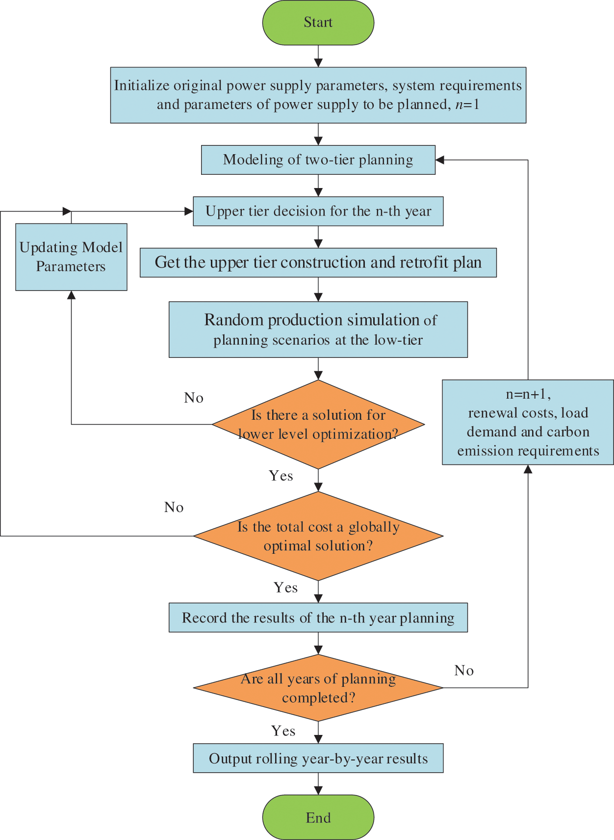
Figure 4: Flowchart of the rolling planning model

5  Analysis of Examples

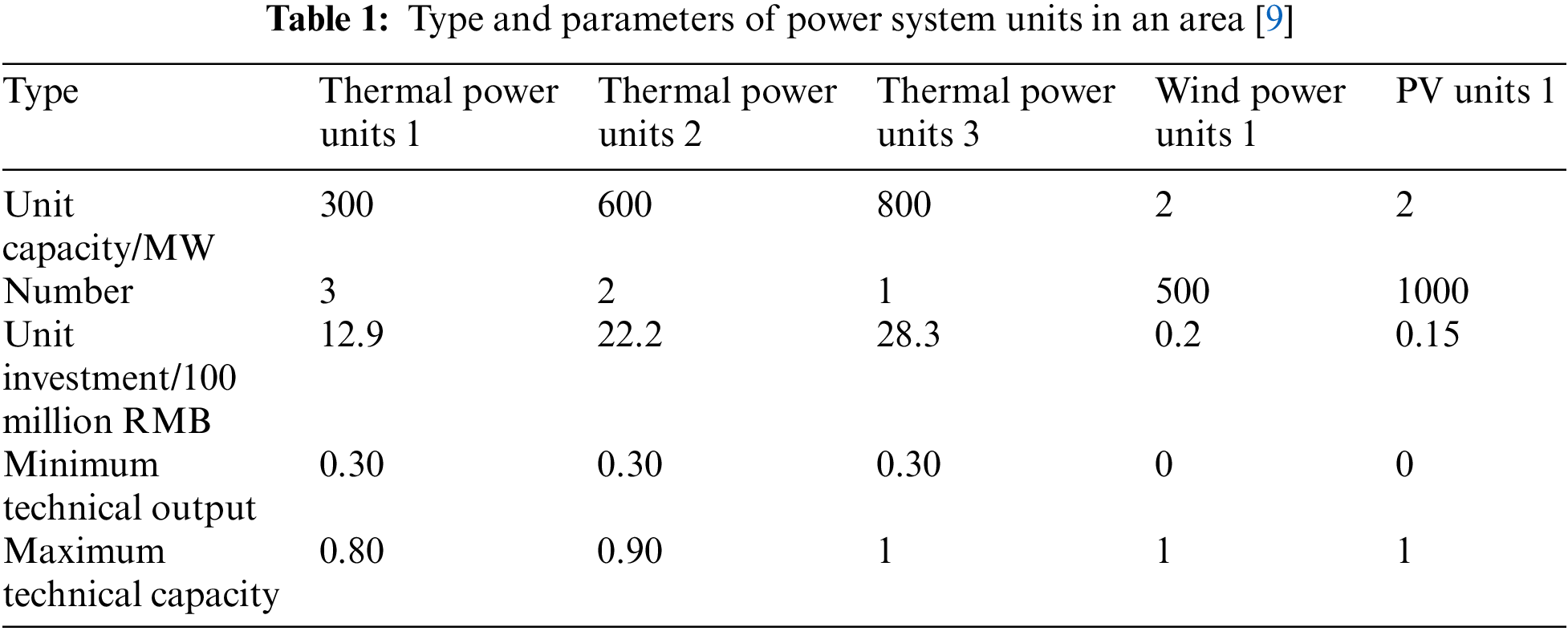
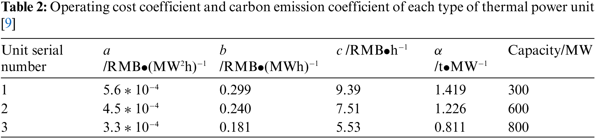
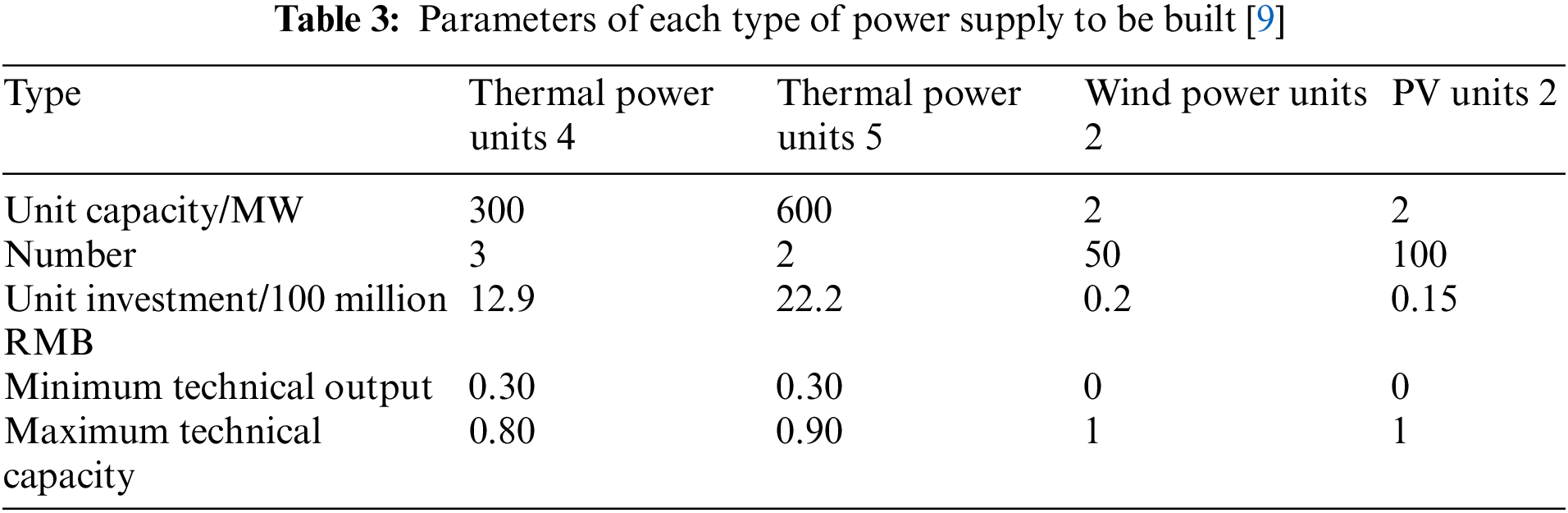
To verify the validity of this model, a small-scale power supply system in a certain region is taken as an example. The rolling planning of thermal power retrofit and generation expansion is conducted to meet the carbon emission target and load demand for the next 5 years, then the planning period is 5 years. The construction time of power units and thermal power retrofit is not considered, and the planned time is assumed to be the time for the thermal unit or the retrofit to be put into service. The peak load demand is 2645 MW with an annual growth rate of 0.08. Before the plan, the region’s annual carbon emissions were 10 million tons, and the plan was to reduce emissions by 5% per year. The original system has no energy storage, and the data are shown in Table 1. The operating cost coefficient and carbon emission coefficient of thermal power are shown in Table 2 [9]. Data of units to be planned are shown in Table 3. The upper limit of allocation energy storage is 2000 MW. For the energy storage, the investment cost is 972 million RMB/MW, the operating cost is 2.2377 RMB/MW, the charging and discharging efficiency is 0.85, and the safe storage power is 0.1–0.9 times the capacity.

When configuring CCS equipment for ordinary thermal power units, the increase in investment and construction cost is 18.6% of the construction cost of the unit itself [11]. The retrofit of new thermal power units is carried out simultaneously with its construction, and the retrofit cost is lower than that of the original unit, so it is set at 0.46% of the construction cost in this paper. In this paper, β is set at 85%, γ is set at 0.08, and the growth rate and εop of each power supply construction cost are set at 1%/year.

5.1 Rolling Decision Result

To reduce the amount of calculation, 12 typical days are selected to verify that the model passed scheme 1: considering carbon emission and power balance risk. The decision results are shown in Figs. 5, 6 and Table 4.

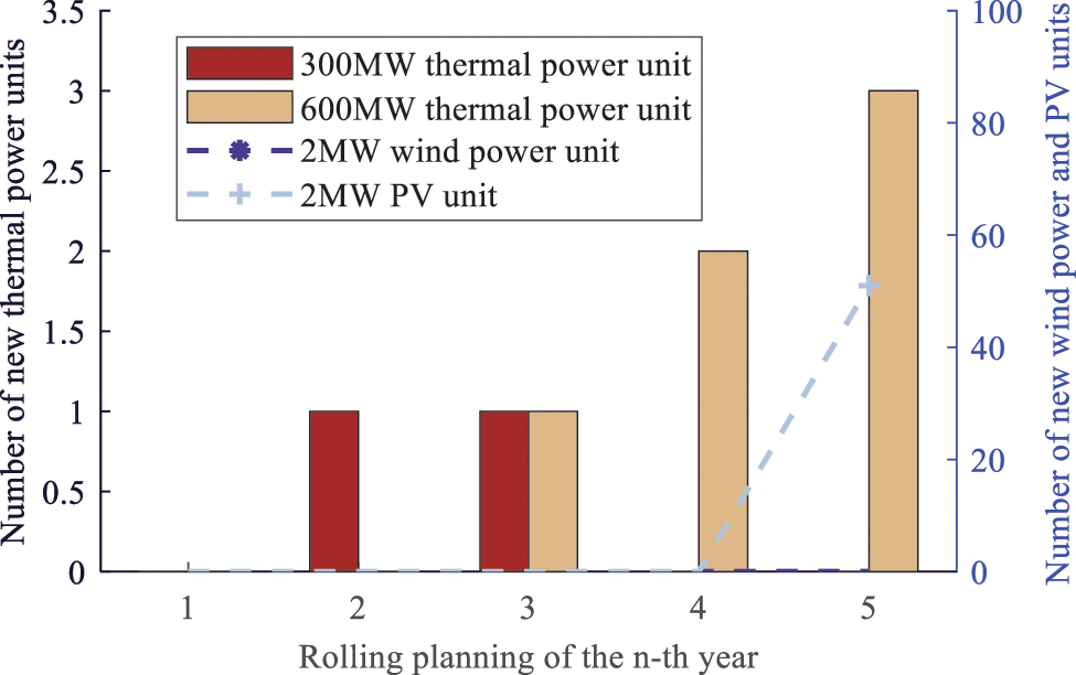
Figure 5: Scheme 1 creates different types each year

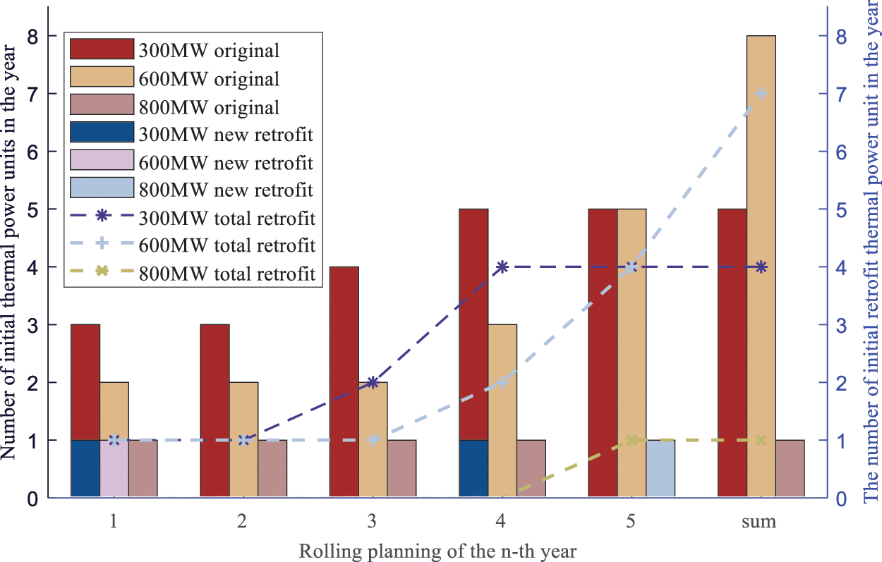
Figure 6: Scheme 1 the number of original thermal power units and conversions at the beginning of each year

Combined with the data in Figs. 5 and 6, it can be seen that due to the intermittence and fluctuation of the output of the wind power and PV units, to ensure the safety of the system operation, the power supply core of the power supply system is still the thermal power unit. When the load demand is relatively low and the emission reduction pressure is small, the construction of small-capacity thermal power units is gradually invested, and new thermal power units are directly retrofitted to reduce the retrofit expenditure as much as possible. Only when the system load demand is high and the emission reduction pressure is greater because most of the thermal power units have been reformed with carbon capture, the effective power supply be less, the zero-emission PV units will be built, and the decision-making cost will be reduced as much as possible while making up for the load demand gap. The reasons for the low capacity of renewable energy construction have two main effects. First, the power supply system has a high proportion of original renewable energy, so there is little demand for renewable energy construction. Secondly, due to the high volatility of renewable energy output, excessive construction of renewable energy can lead to increased power balance risks.

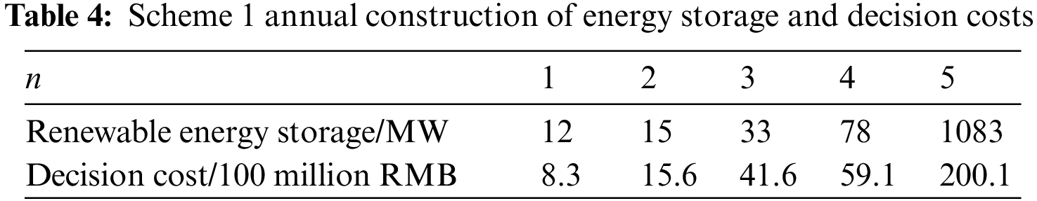
It can be seen from Table 4 that to reduce the risk of power balance, when the original thermal power units start to be gradually retrofitted and the number of new thermal power units is small, the system’s renewable energy absorption capacity decreases slightly, and a small amount of energy storage starts to be built. In the rapid advance of the original thermal power units retrofit, almost all new thermal power units are CCS units, and when the PV unit is built, the system’s renewable energy consumption capacity rapidly declines, and energy storage is then built in large quantities. As can be seen from the change of decision cost data in Table 4, with the gradual expansion and retrofit of the power system and the increase of annual investment and construction costs, the decision cost increases in a rolling step manner. Two of the jump nodes are the third year of thermal power unit construction, retrofit surge, and the fifth year of energy storage, PV investment surge. In the following, the difference between the decision results of scheme 1 and other schemes is compared, and the influence of carbon emission and power balance risk on rolling decisions is analyzed.

5.2 Risks Assessment Analysis

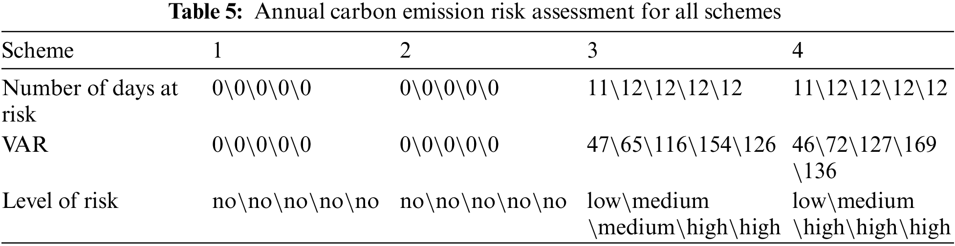
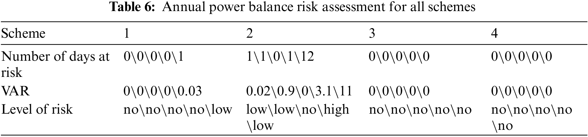
To analyze the impact of considering carbon emission and power balance risk on the economy and security of decision-making, in addition to scheme 1, the following schemes are set up in this paper for comparative analysis: ① Scheme 2 only considers carbon risk; ② Scheme 3 only considers the power balance risk; ③ Scheme 4 does not consider any risks. The decision cost and risk assessment results for each scheme are shown in Fig. 7 and Tables 5, 6. The value-at-risk (VAR) is presented in the form of a typical daily VAR sum.

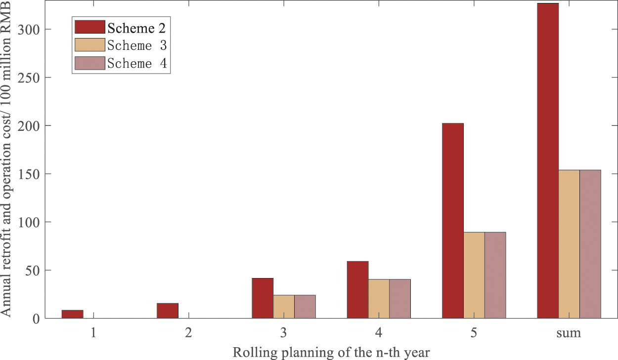
Figure 7: Schemes 1–4 annual decision costs

By comparing the decision cost of schemes 1 and 3 (or 2 and 4), it can be seen that when the load demand is low and the emission reduction pressure is low, the carbon emission risk forces a small amount of thermal power unit retrofit, resulting in the decision cost of the former is higher than the average operating cost of the latter. The average operating cost is about 500 million RMB, which can be almost ignored in Fig. 6. With the increase of emission reduction pressure, the impact of carbon emission risk becomes prominent, and the decision cost of the former is much higher than that of the latter, and the rolling decision cost is almost twice that of the latter.

By comparing the decision cost of options 1, 2 (or 3, or 4), it can be seen that when the load demand is low and the emission reduction pressure is low, the power balance risk has little influence on the decision. With the increase of emission reduction pressure, the impact of considering the power balance risk is still small. Because, in the comparison scheme, the former reduces the wind power unit and PV unit investment and construction, mainly the construction of energy storage, while the latter reduces the energy storage investment and construction, mainly the construction of wind power and PV unit to supplement the power supply so that the final annual decision cost of the two is almost the same.

Through the comparison of different risk data in Tables 5 and 6, it can be seen that although considering carbon emission risk greatly reduces the number of days and risk size of carbon emission risk, it increases the risk of power balance to a certain extent, resulting in the risk of power balance for the system that can perfectly absorb wind power and PV unit power. Considering the power balance risk decision can effectively reduce the risk days and risk size, but its impact on carbon emission risk is very small. The reason is that the thermal power unit capacity of the original system is sufficient, and the proportion of wind power and PV units is small. Only when the risk of carbon emissions is considered, a large number of thermal power units is retrofitted. Then, the actual supply capacity decreases, the proportion of wind power and PV unit power supply increases, and the system absorption capacity decreases, resulting in power balance risk. And, considering the power balance risk does not affect the system output ratio, and does not affect the retrofit of the thermal power unit, its impact on carbon emission risk can be almost ignored.

5.3 Analysis of Influencing Factors of Thermal Power Transformation and Carbon Emission Reduction Efficiency

In this paper, by changing the annual carbon emission constraint of scheme 1 and only making the decision of the first year of the original wind power and PV unit installed capacity, the thermal power unit retrofit capacity and the actual carbon emission evolution curve are observed, and then the factors affecting the thermal power unit retrofit and carbon emission reduction efficiency are analyzed. The results are shown in Figs. 8 and 9.

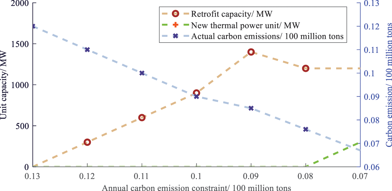
Figure 8: Thermal power unit retrofit and carbon emission evolution curves under different carbon emission constraints

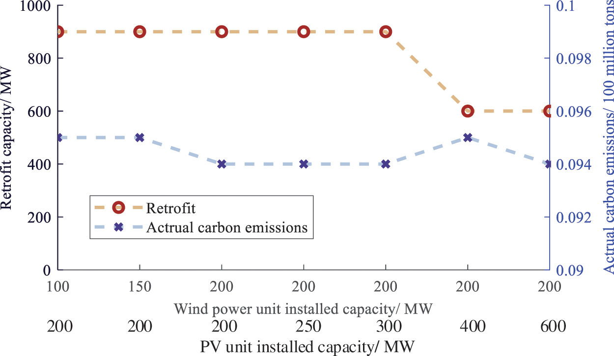
Figure 9: Thermal power unit retrofit and carbon emission evolution curves under different capacities of original renewable energy

As can be seen from Fig. 8, with the reduction of annual carbon emission constraint, the retrofit capacity of thermal power units gradually increases, and the actual carbon emission is significantly reduced, indicating that the main factor affecting the effect of thermal power unit retrofit and emission reduction is the annual carbon emission constraint, that is, the planning requirements for emission reduction. When the annual carbon emission constraint is reduced to a certain extent, the retrofit capacity reaches saturation, indicating that the large-capacity CCS unit can have sufficient carbon emission risk margin under the premise of satisfying the power supply and achieving the emission reduction target under the high emission reduction requirements.

Fig. 9 shows that the installed capacity of renewable energy has little impact on carbon capture retrofit and carbon emissions, and only when the installed capacity of renewable energy is large enough, the retrofit capacity will change slightly. The reason why the retrofit capacity is not sensitive to the change in the installed capacity of renewable energy may also be that the volume of the power system is too small.

6  Conclusions

In this paper, carbon comprehensively considering emission risk and power balance risk, risk assessment indicators and methods are established, and considering risk indicators and factors of thermal carbon capture retrofit based on traditional power supply planning, a two-tier model of rolling decision of power supply planning is established. The following conclusions are obtained through numerical simulation:

1) Considering carbon emissions risk can significantly reduce the number of days of carbon emissions risk and ensure that the power balance risk is within the safe limit. However, the cost of the decision will roll up quickly.

2) Considering carbon emission risk, thermal power unit retrofit reduces thermal power transmission power, transfers the power supply center from thermal power unit to renewable energy generation, and brings power balance risk. Therefore, when considering the carbon emission risk, it is necessary to consider the power balance risk and improve the emission reduction efficiency and economy of the power system while maintaining reliability and stability.

3) The main factor affecting thermal power unit retrofit is the annual carbon emission constraint, that is, the requirements of the annual emission reduction plan. The impact of renewable energy capacity is minimal.

In the future study, the sensitivity of the retrofit capacity to the change of the installed capacity of renewable energy can be tested through a large power supply system, and other emission reduction means can be considered to realize the planning of low-carbon power supply.

Acknowledgement: None.

Funding Statement: This work is supported by Science and Technology Project of State Grid Anhui Electric Power Co., Ltd. (No. B6120922000A).

Author Contributions: Methodology, D.P., and X.G.; software, J.X., and Y.S.; validation, Y.M.; data curation, H.X.; writing—original draft preparation, H.X., and Y.M. All authors have read and agreed to the published version of the manuscript.

Availability of Data and Materials: The data used to support the findings of this study are available from the corresponding author upon request.

Conflicts of Interest: The authors declare that they have no conflicts of interest to report regarding the present study.

References

1. Xu, G., Jiang, X., Xie, Y., Zhang, Z., Bai, D. (2022). Two-step strategy to achieve “double carbon” and method analysis of annual carbon reduction of 100 million tons. China Development, 22(2), 3–11 (In Chinese). [Google Scholar]

2. Zhong, J., Wang, Y., Zhao, Z., Zhang, X. (2020). Research on multi-objective robust optimization about low carbon generation expansion planning considering uncertainty. Acta Energiae Solaris Sinica, 41(9), 114–120 (In Chinese). [Google Scholar]

3. Han, F., Zeng, J., Lin, J., Gao, C., Ma, Z. (2023). A novel two-layer nested optimization method for a zero-carbon island integrated energy system, incorporating tidal current power generation. Renewable Energy, 218, 119381. [Google Scholar]

4. Lin, X., Huang, G., Zhou, X., Zhai, Y. (2023). An inexact fractional multi-stage programming (IFMSP) method for planning renewable electric power system. Renewable and Sustainable Energy Reviews, 187, 113611. [Google Scholar]

5. Zhu, J., Wang, M., Sui, B., Wu, H., Fu, K. et al. (2022). Research on power expansion planning under low carbon economy. 2022 7th Asia Conference on Power and Electrical Engineering (ACPEE), pp. 1125–1130. Hangzhou, China. [Google Scholar]

6. Zhang, X., Yan, P., Zhong, J., Lu, Z. (2015). Research on generation expansion planning in low-carbon economy environment under incentive mechanism of renewable energy sources. Power System Technology, 39(3), 655–662 (In Chinese). [Google Scholar]

7. Wang, C., Yun, F., Ning, L. (2016). Research on generation expansion planning in low-carbon economy environment based on multi-scenario technique. Electric Power, 49(S1), 102–106 (In Chinese). [Google Scholar]

8. Norişor, M., Cenuşă, V. E., Arion, E. (2017). The impact of using the post-combustion CCS on the coal-fired TPP internal consumptions. 10th International Symposium on Advanced Topics in Electrical Engineering (ATEE), pp. 559–562. Bucharest, Romania. [Google Scholar]

9. Lu, Z. G., Feng, T., Li, X. P. (2013). Low-carbon emission/economic power dispatch using the multi-objective bacterial colony chemotaxis optimization algorithm considering carbon capture power plant. International Journal of Electrical Power & Energy Systems, 53, 106–112. [Google Scholar]

10. Chen, Q., Kang, C., Xia, Q. (2010). Operation mechanism and peak-load shaving effects of carbon-capture power plant. Proceedings of the CSEE, 30(7), 22–28 (In Chinese). [Google Scholar]

11. Ji, Z., Chen, Q., Zhang, N., Li, H., Huang, J. et al. (2013). Low-carbon generation expansion planning model incorporating carbon capture power plant. Power System Technology, 37(10), 2687–2696 (In Chinese). [Google Scholar]

12. Ma, Y., Liu, C., Yang, H., Zhang, D. (2023). Robust optimization of unit commitment with wind power considering composite flexibility constraints. International Journal of Electrical Power & Energy Systems, 151, 109146. [Google Scholar]

13. Yang, B., Guo, Z., Wang, J., Duan, C., Ren, Y. et al. (2022). Key optimization issues for renewable energy systems under carbon-peaking and carbon neutrality targets: Current states and perspectives. Energy Engineering, 119(5), 1789–1795. [Google Scholar]

14. Huang, H., Wang, Y., Liu, S., Wang, S., Tang, L. et al. (2023). Stochastic generation and transmission expansion planning considering the correlation between load and wind power output. 2023 8th Asia Conference on Power and Electrical Engineering (ACPEE), pp. 365–369. Tianjin, China. [Google Scholar]

15. Abaul, H., Muhammad, M. A., Ammar, A. (2023). Emission constrained generation expansion planning considering site-dependent renewable energy sources of Pakistan. 2023 International Conference on Emerging Power Technologies (ICEPT), pp. 1–6. Topi, Pakistan. [Google Scholar]

16. Zhou, H., Liang, L., Shen, L., Wang, Q., Zhang, H. et al. (2023). A study on source-network-demand coordinated expansion planning of the sending power system considering DC transmission and hydro-solar complementary. 2023 Panda Forum on Power and Energy (PandaFPE), pp. 1902–1908. Chengdu, China. [Google Scholar]

17. Shang, H., Liu, T., Bu, T., He, C., Yin, Y. et al. (2020). Operational risk assessment of power system considering wind power and photovoltaic grid connection. Modern Electric Power, 37(4), 358–367. [Google Scholar]

18. Zhang, G., Li, F. (2022). Two-stage optimal dispatch for wind power integrated power system considering operational risk and reserve availability. Power System Protection and Control, 50(11), 139–148 (In Chinese). [Google Scholar]

19. Ma, R., Xiong, L. (2012). Power system economic dispatching considering the impact of wind powers and loads uncertainty. Journal of Electric Power Science and Technology, 27, 41–46. [Google Scholar]

20. Baradar, M., Hesamzadeh, M. R. (2014). A stochastic SOCP optimal power flow with wind power uncertainty. 2014 IEEE PES General Meeting | Conference & Exposition, National Harbor, pp. 1–5. MD, USA. [Google Scholar]

21. Dhayalini, K., Mukesh, R. (2019). Optimal setting and sizing of distributed solar photovoltaic generation in an electrical distribution system. 2019 Innovations in Power and Advanced Computing Technologies (i-PACT), 1,1–5. [Google Scholar]

22. Fazlalipour, P., Ehsan, M., Mohammadi-Ivatloo, B. (2018). Risk-aware stochastic bidding strategy of renewable micro-grids in day-ahead and real-time markets. Energy, 171, 689–700. [Google Scholar]

23. Ma, Y., Zhang, M., Wang, X., Xu, J., Hu, X. (2023). Decentralized and coordinated scheduling model of interconnected multi-microgrid based on virtual energy storage. International Journal of Electrical Power & Energy Systems, 148, 108990. [Google Scholar]

24. Miguel, C., Jose, M. A. (2006). A computationally efficient mixed-integer linear formulation for the thermal unit commitment problem. IEEE Transactions on Power Systems, 21(3), 1371–1378. [Google Scholar]

25. Feron, P., Abu-Zahra, M., Alix, P. (2007). Development of post-combustion capture of CO2 within the CASTOR integrated project: Results from the pilot plant operation using MEA. The 3th International Conference on Clean Technologies for Our Future, pp. 1268–1275. Sardinia, Italy. [Google Scholar]

26. Liu, Y., Guo, L., Wang, C. (2018). Economic dispatch of microgrid based on two stage robust optimization. Proceedings of the CSEE, 38(14), 4013–4022+4307 (In Chinese). [Google Scholar]