
 Submit a Paper
 Propose a Special lssue
 Open Access
ARTICLE

Thermal Performance and Economic Efficiency Comparison of Typical Shallow and Medium-Deep Borehole Heat Exchanger Heating Systems in Xi’an, China
1 Key Laboratory of Coal Resources Exploration and Comprehensive Utilization, Ministry of Natural Resources, Xi’an, 710021, China
2 Shanghai Engineering Research Center for Shallow Geothermal Energy, Shanghai, 200072, China
3 Shanghai Geological Engineering Exploration (Group) Co., Ltd., Shanghai, 200072, China
4 School of Human Settlements and Civil Engineering, Xi’an Jiaotong University, Xi’an, 710049, China
5 Lee Kong Chian Faculty of Engineering and Science, Universiti Tunku Abdul Rahman, Kajang, 43000, Selangor, Malaysia
* Corresponding Authors: Guosheng Jia. Email: ; Lip Huat Saw. Email:
Energy Engineering 2025, 122(3), 1005-1024. https://doi.org/10.32604/ee.2025.059198
Received 30 September 2024; Accepted 26 December 2024; Issue published 07 March 2025
 View Full Text
 Download PDF
Abstract
Geothermal energy, a form of renewable energy, has been extensively utilized for building heating. However, there is a lack of detailed comparative studies on the use of shallow and medium-deep geothermal energy in building energy systems, which are essential for decision-making. Therefore, this paper presents a comparative study of the performance and economic analysis of shallow and medium-deep borehole heat exchanger heating systems. Based on the geological parameters of Xi’an, China and commonly used borehole heat exchanger structures, numerical simulation methods are employed to analyze performance and economic efficiency. The results indicate that increasing the spacing between shallow borehole heat exchangers can effectively reduce thermal interference between the pipes and improve heat extraction performance. As the flow rate increases, the outlet water temperature ranges from 279.3 to 279.7 K, with heat extraction power varying between 595 and 609 W. For medium-deep borehole heat exchangers, performance predictions show that a higher flow rate results in greater heat extraction power. However, when the flow rate exceeds 30 m3/h, further increases in flow rate have only a minor effect on enhancing heat extraction power. Additionally, the economic analysis reveals that the payback period for shallow geothermal heating systems ranges from 10 to 11 years, while for medium-deep geothermal heating systems, it varies more widely from 3 to 25 years. Therefore, the payback period for medium-deep geothermal heating systems is more significantly influenced by operational and installation parameters, and optimizing these parameters can considerably shorten the payback period. The results of this study are expected to provide valuable insights into the efficient and cost-effective utilization of geothermal energy for building heating.Graphic Abstract

Keywords
Nomenclature
| A | Cross-sectional area of the flow section, m2 |
| AO,I | Inner surface area of the outer pipe, m2 |
| Cp,w | Water specific heat capacity, J/(kg·°C) |
| Dd | Asset depreciation rate, % |
| DO,i | Inner diameter of the outer pipe, m |
| DO,o | Outer diameter of the outer pipe, m |
| Ea | Annual heat extraction amount, kWh |
| Ff | Flow friction, N/m3 |
| g | Gravitational acceleration, m/s2 |
| hann | Convective heat transfer coefficient, W/(m2·°C) |
| kpipe,O | Thermal conductivity of the outer pipe, W/(m2·°C) |
| LCOE | Levelized cost of energy, RMB/GJ |
| M | Mass flow rate of the working fluid, kg/s |
| PBP | Payback period, year |
| p | Pressure, Pa |
| Pd | Construction cost, RMB |
| PO&M | Operating cost, RMB |
| q | Heat extraction power, W |
| Qs | Total heat flux, W/m2 |
| r | Radial coordinate, m |
| Rann | Convective thermal resistance, °C/W |
| Rd | Depreciation rate, % |
| Rpipe,O | Convective thermal resistance of the outer pipe, °C/W |
| Rtax | Tax rate, % |
| ST | Energy source term, N/m3 |
| Su | Momentum source term, N/m3 |
| t | Time, s |
| △T | Inlet and Outlet temperature difference, °C |
| Tbulk | Average temperature of the water in the cross-section, °C |
| TO&M | Full lifecycle, year |
| TO,o | Outer wall temperature of the outer pipe, °C |
| Ts | Ground surface temperature, °C |
| u | Average flow velocity of the water, m/s |
| Vr | Salvage value, RMB |
| x | Axial coordinate, m |
| ρw | Water density, kg/m3 |
Scholars from various countries are committed to finding effective, clean, and sustainable new energy sources and promoting their efficient utilization [1–3]. Due to its widespread distribution and vast reservoirs, geothermal energy has garnered substantial interest [4–6]. In recent years, researchers from multiple nations have consistently focused on the effective use of geothermal energy [7–10]. A common method of geothermal energy utilization involves circulating a working fluid (usually water) within a closed-loop borehole heat exchanger (BHE), such as U-tube or coaxial heat exchangers, to absorb heat from the adjacent rock and soil and convey it to surface equipment [11–13]. In terms of the burial depth, BHEs in geothermal heating systems are categorized as shallow BHEs (tens to hundreds of meters) and medium-deep BHEs (2000 to 3000 m) [14,15]. Shallow BHE systems typically use numerous BHEs, ranging from tens to hundreds of meters in depth. These systems predominantly employ U-tube heat exchangers to transfer heat with subterranean rock formations, providing heating in winter and cooling in summer. Conversely, medium-deep buried pipes harness geothermal energy from rock strata located 2 to 3 kilometers below the surface, where temperatures range from 70°C to 90°C or higher, serving as the thermal source for heat pump systems [16].
Currently, there are various methods for forecasting the efficacy of borehole heat exchangers (BHEs). These methods can be categorized into analytical methods and numerical methods, such as the finite element method, finite difference method, and others. Early analytical models for theoretical calculations can be traced back to 1948, when Ingersoll [17] studied and developed the line heat source model suggested by Kelvin [18] in 1882, providing a solution for radial heat transfer in BHEs. Claesson et al. [19] were the pioneers in presenting an analytical solution for a finite line source (FLS). In addition to analytical solutions, many researchers have employed numerical methods based on discretization and grid division of the computational domain to study various types of BHEs. For example, Yu et al. [20] established a segmented numerical calculation model for U-shaped BHEs with large pipe spacing. Their model studied depths of up to 500 m with pipe spacing of 200 m. Hecht et al. [21] used FEFLOW to model and simulate a group of 25 U-shaped BHEs buried to a depth of 100 m. Gordon et al. [22] proposed a semi-analytical calculation model for composite cylindrical heat sources. This model is founded on existing cylindrical heat source theory and interprets the temperature response generated by the heat exchanger as the superposition of three components: heat conduction in the surrounding ground, the grout layer, and the outer wall of the heat exchanger, resulting in an overall temperature response. Moreover, the work proposed by Mahariq et al. [23] suggested that the spectral element method (SEM), a numerical approach integrating spectral methods with the finite element method, may be utilized in forthcoming investigations owing to its superior accuracy.
The main challenges in geothermal energy development include high initial investment costs. These costs are particularly evident in the various stages of deep ground layer development, including site preparation, drilling, and pipeline installation. Therefore, conducting an economic analysis of medium-deep geothermal heating systems is essential. Lu et al. [24] assessed the economic performance of vertical ground source heat pump (GSHP) systems in residential settings in Melbourne, Australia, using several economic indicators. Buonomano et al. [25] researched the design, simulation, and optimization of geothermal and solar power plants. Their findings demonstrated that the thermal efficiency of geothermal and solar systems is more contingent upon the availability of geothermal energy than on solar energy. Under the most adverse operating conditions, the investment payback period was 7.6 years, which is shorter than that of boiler heating systems. Blum et al. [26] explored the technical and economic parameters affecting the design and operation of GSHP systems, evaluating their relationship with geographical factors such as geology and climate. They analyzed data from over 1,100 GSHP systems, concluding that the average capital expenditure for these systems in Germany is approximately €23,500 ± €6,800, with 51% of the cost attributable to drilling operations. Danilidis et al. [27] developed an economic model for a deep geothermal system. The findings revealed that the costs of drilling constitute the principal capital outlay, and net present value (NPV) is significantly influenced by variables such as discount rates and inflation rates. Xia et al. [28] utilized Monte Carlo simulations and sensitivity analyses to assess the economics of geothermal heating systems. Their results indicated that the economic viability of geothermal heating systems is mostly affected by heating revenue, discount rates, and non-depreciable initial investments.
Due to the high initial investment required for geothermal energy systems, extensive study has been undertaken on the performance forecasting of BHEs, the factors that influence their efficiency, and their long-term operational effectiveness. These studies provide a theoretical foundation for the effective utilization of geothermal energy. Nonetheless, there is an absence of economic analysis regarding geothermal energy systems, particularly comprehensive studies on the performance and economics of medium-deep and shallow geothermal systems in specific regions. This gap limits informed decision-making in practical engineering applications for these two systems.
This paper focuses on a comparative analysis of the thermal and economic performance of shallow and medium-deep BHE heating systems. Using geological parameters from Xi’an, China, the study examines the factors influencing performance and the thermal variation patterns of typical-sized shallow U-tube buried pipes and medium-deep coaxial heat exchangers during long-term operation, through numerical simulations. The economic analysis covers the investment payback period (PBP) and the levelized cost of energy (LCOE) over extended operation, emphasizing the thermal and economic trends of both systems. The suggested optimization strategies for system design aim to serve as a theoretical foundation for decision-makers choosing between shallow and medium-deep systems. Furthemrore, this work offers a comprehensive evaluation method that integrates thermal and economic performance considerations.
2 Methods for BHE Thermal Performance Analysis
In this section, a model incorporating typical geological parameters, structural parameters, and operating conditions of a shallow BHE array is established. The geological parameters include the soil’s density, specific heat capacity, and thermal conductivity. The structural parameters encompass the diameter, drilling depth, and pipe spacing of the BHEs. The operating conditions refer to the fluid velocity within the BHE and the inlet temperature. The ICEM (Integrated Computer Engineering and Manufacturing) software is employed to construct the geometric model of the BHE array and generate the mesh. Heat conduction transpires between the underground pipes and the earth during the heat transfer process, accompanied by turbulent flow heat transmission inside the working fluid. Simultaneously, heat exchange takes place among the backfill material, the pipes, and the adjacent soil. To ensure the accuracy of model calculations and reduce complexity, the following assumptions are adopted:
1. The thermal conductivity, density, and specific heat capacity of the soil and backfill material remain constant over time and temperature.
2. The initial temperature and thermal characteristics of the soil at the same depth are uniform.
3. Mass transfer between the soil and backfill material is neglected.
As shown in Fig. 1, the buried pipes are arranged in a square layout of 6 × 6, with pipe spacings of 4, 6, and 8 m. The surrounding soil width of the pipe array is 20 m. For ease of analysis and discussion, the buried pipes in the upper right corner are numbered sequentially from 1 to 9. The arrangement of the pipe array and its overall dimensions are summarized in Table 1.
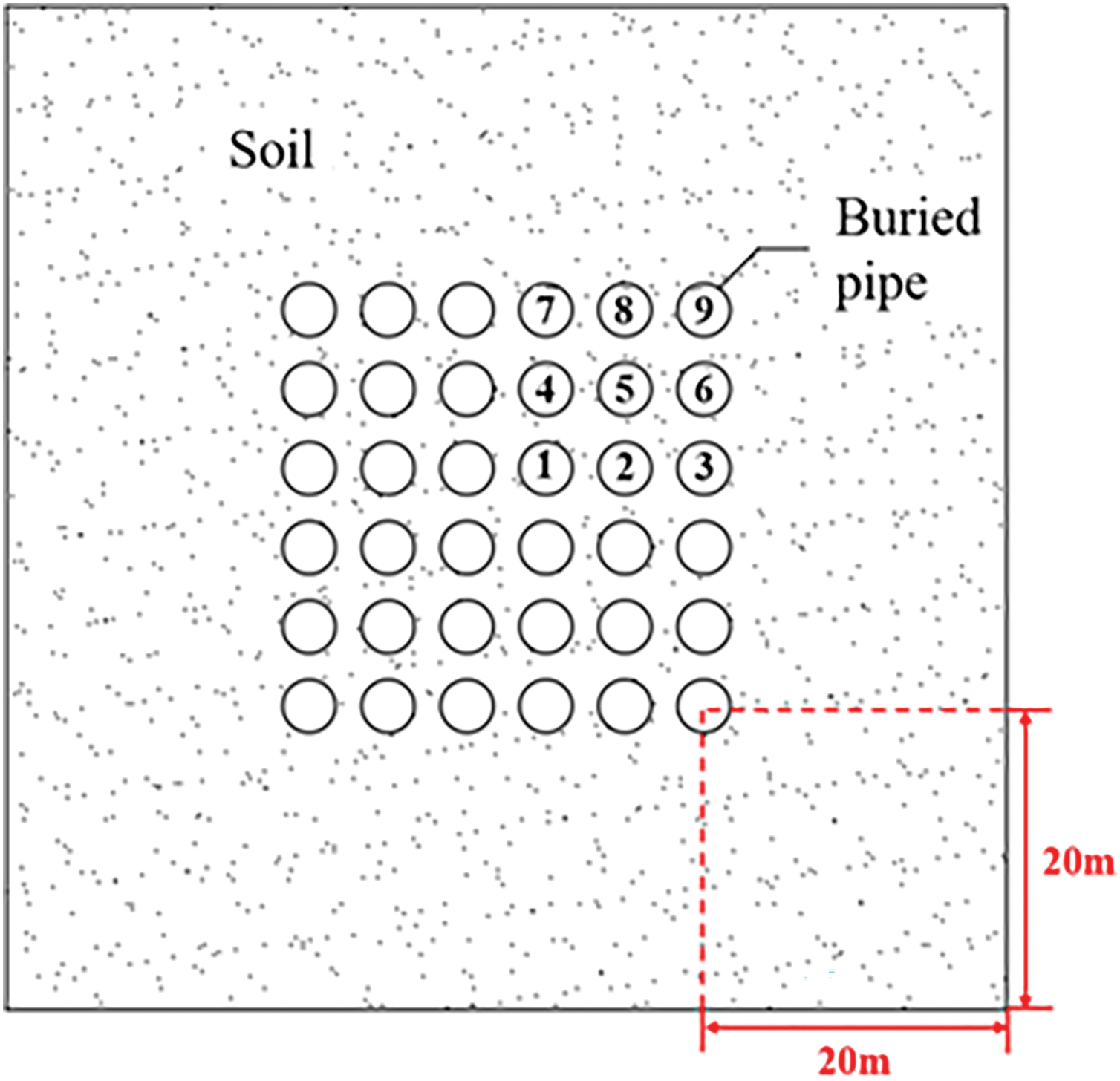
Figure 1: Diagram of shallow BHE array layout

Due to the symmetry of the BHE array distribution, one-quarter of the model shown in Fig. 1 is selected for meshing. The BHE distances are set to 6 and 4 m, respectively. The mesh for the U-shaped BHE is illustrated in Fig. 2. Based on engineering experiments, water is designated as the working fluid within the U-shaped pipe. The flow state within the pipe is turbulent, and calculations are performed using the Realizable k-ε model. The U-shaped pipe is made of PE, and the backfill material is chosen to have properties similar to those of the surrounding soil. The specific physical property parameters of the model are based on the shallow soil characteristics in the Xi’an area, as detailed in Table 2. The model’s input parameters comprise the following:
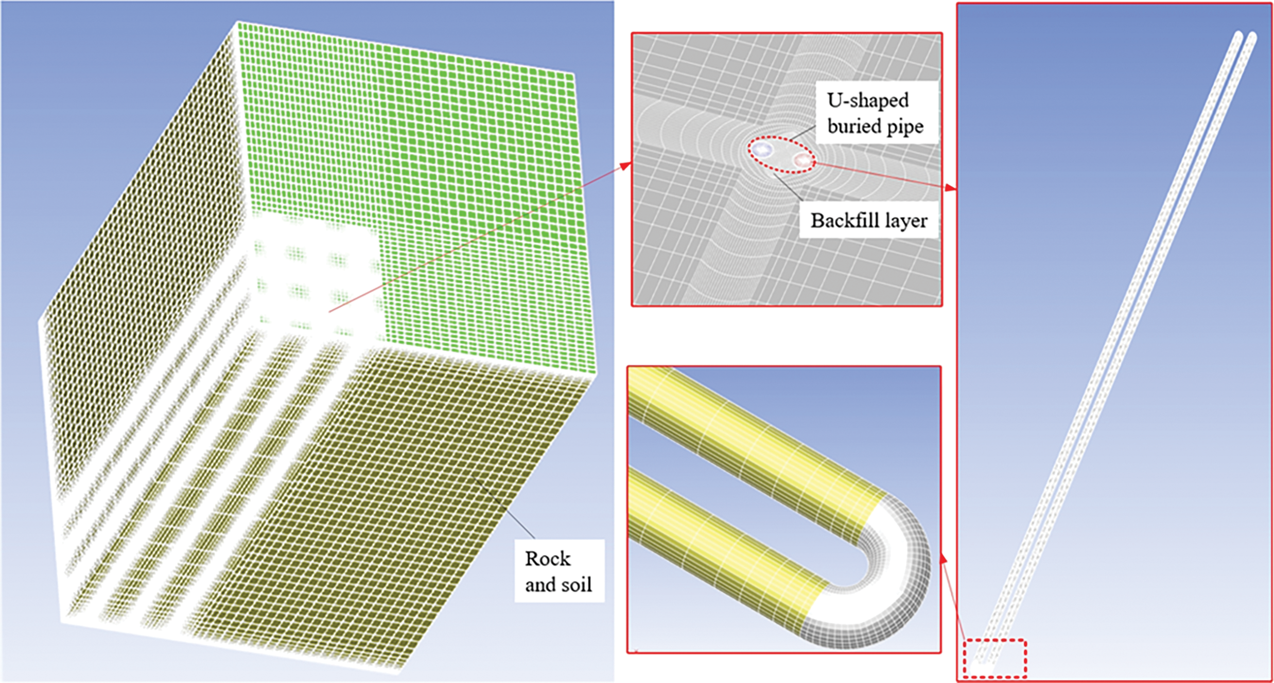
Figure 2: U-shaped heat exchanger mesh establishment

• Inlet flow velocity of the circulating water: 0.4 and 0.7 m/s
• Initial inlet water temperature: 6°C
• Initial ground temperature: 14°C
• Operating time: 120 days
To validate the proposed model, it is compared with the line source analytical solution formulated by Erol et al. [29]. The initial soil temperature is set at 13.85°C, and the flow rate is 0.5 m/s. Fig. 3 depicts the comparison of soil temperatures at distances of 1 and 2 m from the BHE. The findings demonstrate that the predictions from the proposed model align closely with the analytical solution. The maximum deviation is less than 0.2 K, demonstrating the reliability of the proposed model.
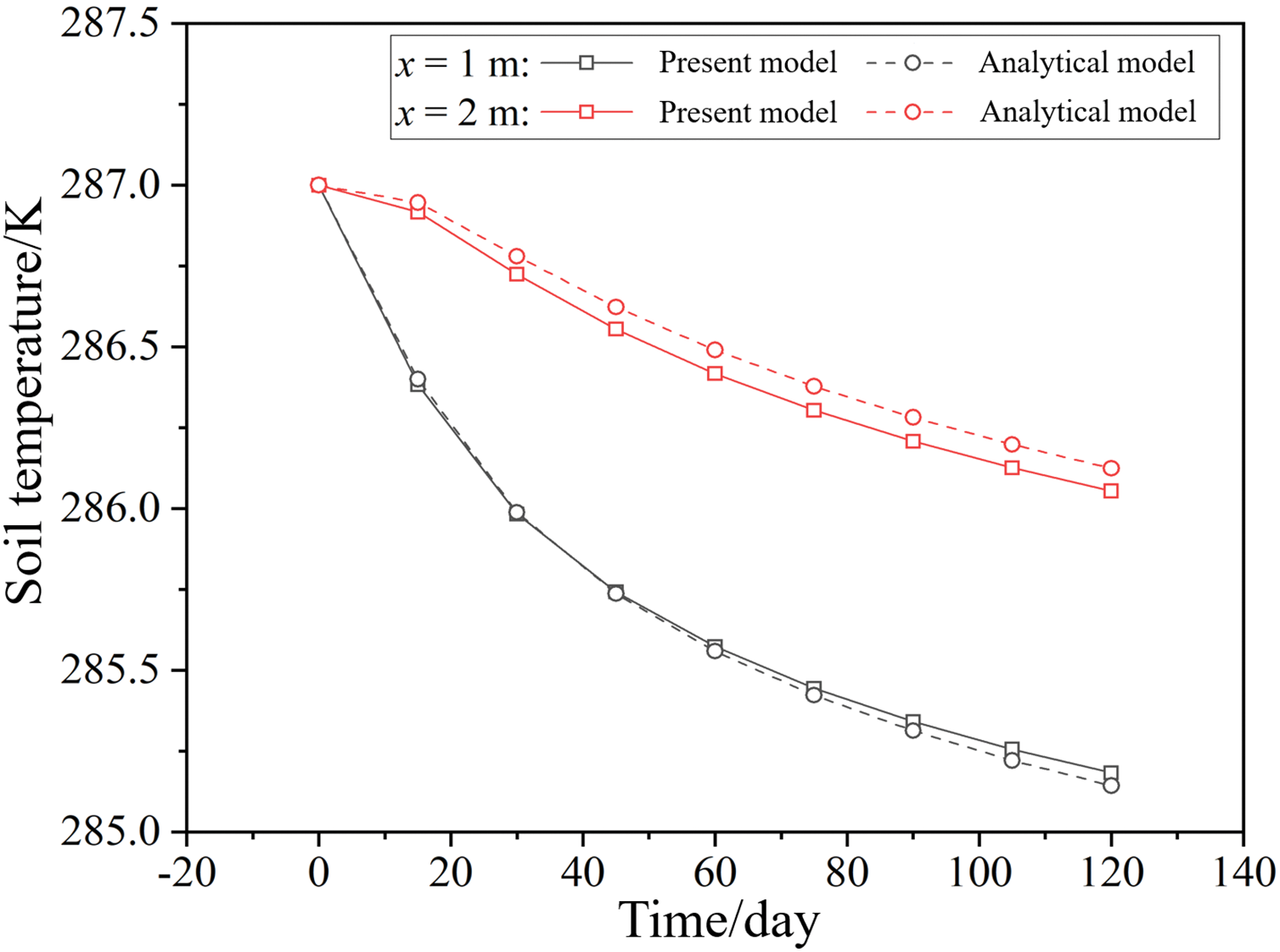
Figure 3: Validation of the shallow BHE model [29]
To rapidly predict the performance of a medium-deep BHE, a full-scale model with a variable control volume is established and solved using the finite volume method (FVM) [30]. The BHE is segmented into several computational segments from top to bottom, with the segment length varying based on the rate of change in geological parameters. This approach effectively reduces computation time while maintaining calculation accuracy. The following assumptions are adopted:
1. The thermal conductivity, density, and specific heat capacity of the soil and backfill material remain constant over time and temperature.
2. The initial temperature and thermal properties of the soil at the same depth are uniform.
3. Mass transfer between the soil and the backfill material is neglected.
4. During operation, heat transport in the central pipe and annulus is presumed to be unidimensional along the axial direction.
5. The ground temperature is presumed to depend only on depth. Due to terrestrial heat flow, the unperturbed temperatures of soil and rock rise with depth; nonetheless, at any given depth, the temperature distribution remains uniform.
The control equations and boundary conditions are defined as follows:
1) The governing equations for the operational state of the BHE are given in [5],
where t is operating time, s. A is the cross-sectional area of the flow part, m2. ρw is the water density, kg/m3. x is the axial coordinate, m. u is the average flow velocity, m/s. p is the average pressure, Pa. Ff is the friction force, N/m3. Su represents the momentum source term, N/m3. g represents the gravitational acceleration, m/s2. Cp,w denotes the water specific heat capacity, J/(kg·°C). T is the water temperature, °C. ST represents the energy source term, W/m3.
The boundary condition for heat conduction is expressed as [5],
where Qs is the total heat flux between the water and the surrounding soil in the control volume, W/m2. Tbulk denotes the average temperature of water at the cross-section, °C. TO,o is the outer wall temperature, °C. Rann is the convective thermal resistance, °C/W. Router is the outer tube thermal resistance, °C/W. r represents the radial coordinate, m. DO,o represents the outer diameter of the outer pipe, m. The convective heat transfer resistance and conductive thermal resistance are calculated using the following two equations, respectively [5],
where hann represents the convective heat transfer coefficient of water, W/(m2·°C). AO,i is the inner wall surface area of the outer pipe, m2. DO,i represents the inner diameter of the outer pipe, m. kpipe,O denotes the heat transfer coefficient of the outer pipe, W/(m2·°C).
The initial temperature condition of the water is as follows:
where the Ts represents the ground surface temperature, °C.
The velocity boundary condition of the water is,
2) The governing equation for the static state of the BHE is [5],
where Cp is the heat capacity, J/(kg·K). λs is the thermal conductivity, W/(m·K). The physical properties represent the characteristics of the materials (water, pipe or soil) at different locations. Similarly, these parameters are calculated sequentially along the depth of the BHE, while neglecting axial thermal diffusion.
When the system is in a static state, the boundary conditions for the energy equation are as follows:
Under static conditions, the initial temperature corresponds to the water temperature at the moment the system equipment is turned off. Therefore, the initial condition can be expressed as,
Based on different operating conditions and durations, the governing equations can be discretized and solved to determine the outlet water temperature of the heat exchanger and the soil temperature distribution at various times and locations.
The developed medium-deep BHE model incorporates commonly used equipment structures and geological parameters specific to the Xi’an region. The borehole depth is 2500 m, with the first section spanning depths from 0 to 500 m and the second section from 500 to 2500 m. The structural parameters for each section are provided in Table 3. The soil temperature gradient is 0.322 °C/km. The heat capacity, density and thermal conductivity of soils and rocks in different depths are detailed in Table 4.


The model was implemented and solved using MATLAB. The calculation process primarily involves the following steps:
1. Inputting the BHE structural and geological parameters.
2. Solving the governing equations (Eqs. (1) to (11)).
3. Outputting the BHE performance parameters.
This process is illustrated in Fig. 4.
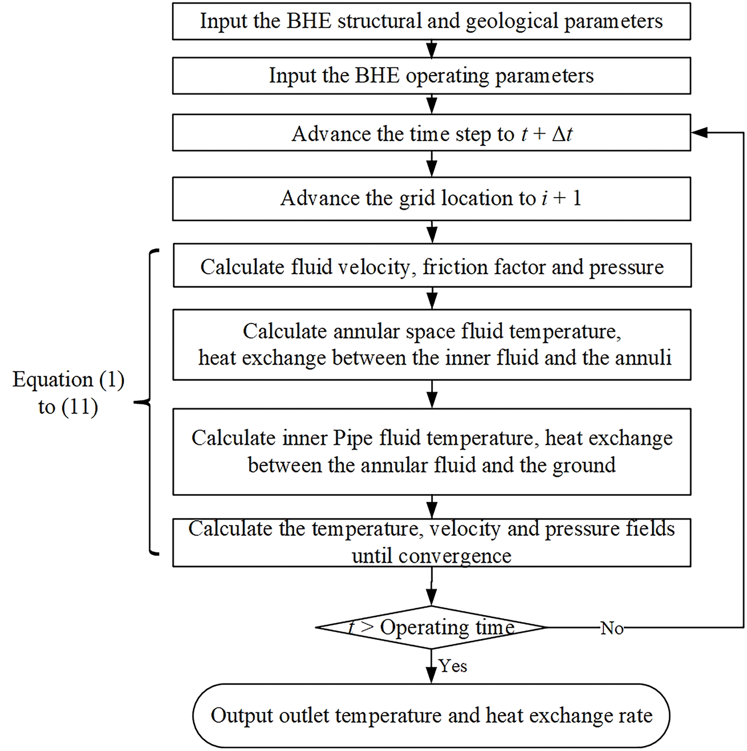
Figure 4: Flow chart of the medium-deep BHE calculation method
The variations in outlet water temperature and heat extraction power of the medium-deep BHE with varying flow rates and operating times are analyzed. The model input parameters include:
• Working fluid volumetric flow rate: 10 to 60 m3/h, in increments of 5 m3/h
• Daily operating time: 8 to 24 h per day, in increments of 4 h
• Inlet water temperature: 15°C
• Total operating time: 120 days
Each flow rate is evaluated under five different operating time scenarios, resulting in a total of 55 operating conditions.
For validation, the proposed model and calculation methods are compared with experimental results from a 2600 m BHE in Qingdao, China [5] (as shown in Fig. 5). During testing, the inlet water temperature was established at 5°C, with a flow rate of 30 m3/h. After 140 days of operation, the comparison indicated that the model precisely forecasts the outlet temperature, with a Root Mean Squared Error (RMSE) of 0.82.
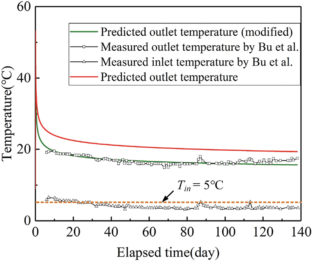
Figure 5: Validation of the medium-deep BHE model [5]
3 Results and Discussion of BHE Thermal Performance
To investigate the thermal interactions among different pipes and the thermal performance of pipes located at various positions within the array, FLUENT program simulates the heat exchange process of a 6 × 6 BHE array and the surrounding soil under long-term operation with different pipe spacings. The results and analysis are as follows:
1) Ground temperature variation characteristics
The heat extraction efficacy of the shallow BHE operating during winter is examined first. The inlet flow velocity of the circulating water is set to 0.6 m/s, with an initial inlet water temperature of 6°C and an initial ground temperature of 14°C. The operating period for the 6 × 6 BHE array is 120 days, corresponding to the heating season in northern China (November 15 to March 15 of the following year). The temperature field distributions are shown in Fig. 6a to f. The thermal interactions among different BHEs become increasingly pronounced as the operating time increases. At a BHE spacing of 4 m, no substantial thermal interaction is detected in the temperature fields after 30, 60, or 90 days of operation. However, after 120 days, as shown in Fig. 6d, noticeable changes in isotherms are evident. As the spacing between the buried pipes increases, as shown in Fig. 6e and f, the thermal interactions significantly decrease. Thus, under the same operating time, increasing the spacing between pipes effectively reduces thermal interactions among BHEs.
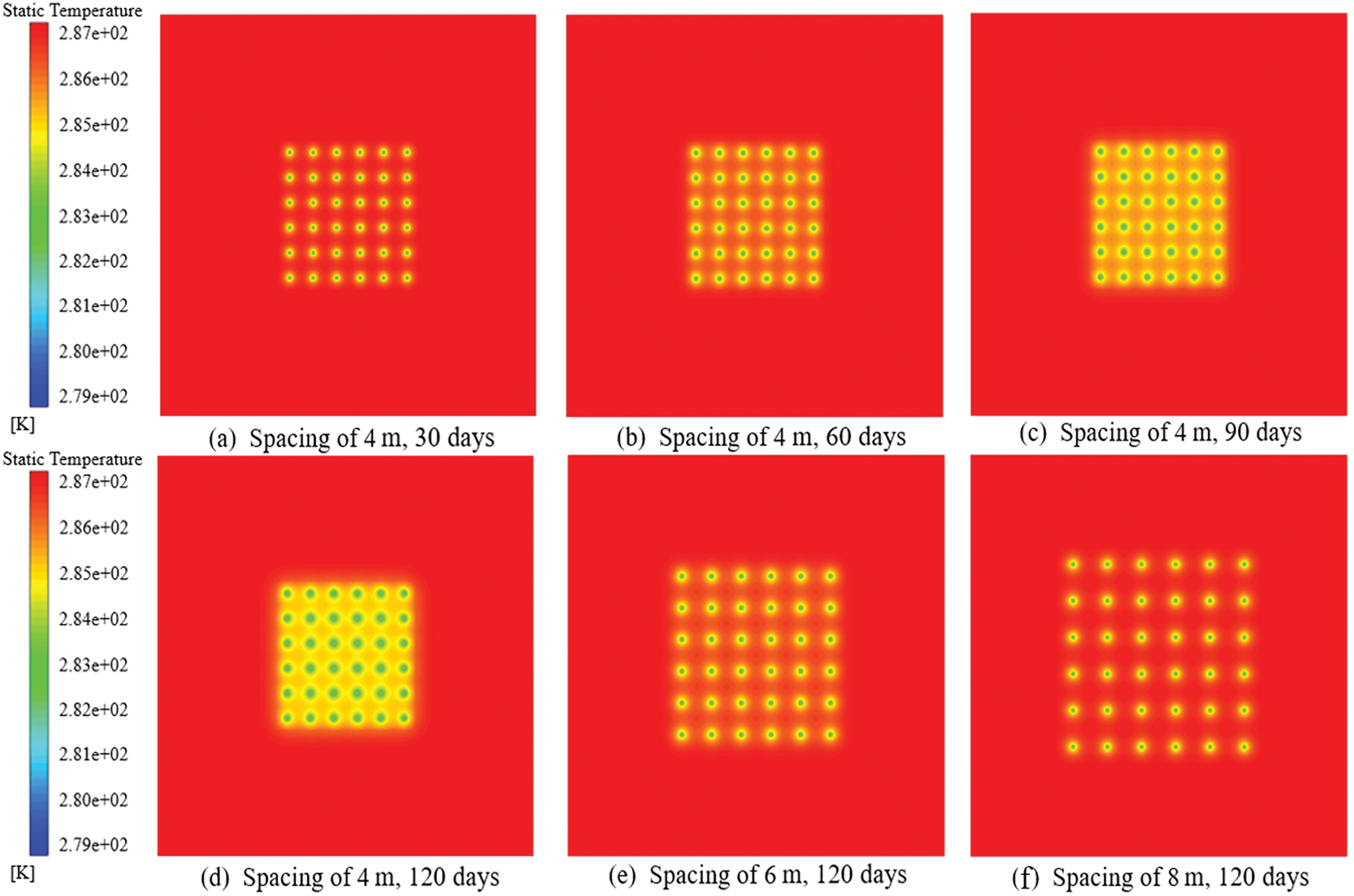
Figure 6: Variation of ground temperature field for shallow BHEs with different pipe spacings
2) Influence of flow velocity on the heat extraction performance
To clarify the effect of the working fluid velocity within the BHE on the ground temperature field and system performance, numerical simulations are conducted under different operating conditions. Using a BHE spacing of 4 m as an example, Fig. 7a and b shows the variation in outlet water temperature at flow velocities of 0.4 and 0.7 m/s, respectively. As the flow velocity increases, the outlet water temperature gradually decreases. This is because a higher flow rate leads to greater heat extraction from the soil. As the BHE absorbs heat from the surrounding soil, the soil temperature diminishes, and heat from the distant high-temperature soil is conveyed to the adjacent low-temperature soil, a phenomenon termed natural geothermal recovery. However, if the BHE’s heat extraction rate exceeds the natural geothermal recovery rate, there will be an insufficient balance of extracted heat, leading to a reduction in ground temperature and a decline in BHE performance.
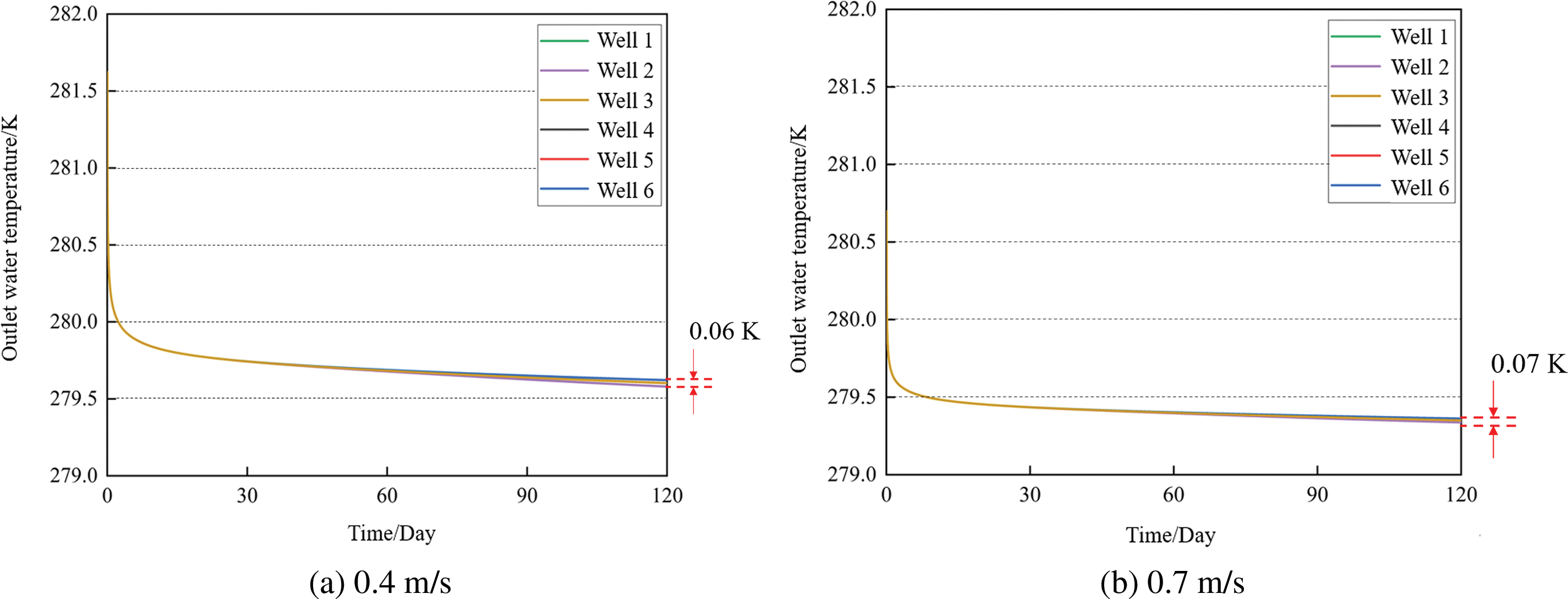
Figure 7: Impact of flow velocity on outlet water temperatures of different BHEs in the array
Besides, the variations in outlet water temperature among the underground pipelines at various places are rather minimal. The maximum deviations in outlet water temperature are observed at flow velocities of 0.4 and 0.7 m/s. The simulation results indicate that augmenting the flow velocity has a negligible impact on the heat extraction efficiency of the BHE. With similar BHE heat extraction rates, the soil temperature field shows the same trend. Therefore, reducing the flow velocity to decrease thermal interaction is not advisable.
To more clearly compare the influence of BHE spacing on BHE performance and to investigate the variations in outlet water temperature and heat extraction power among BHEs at various positions within the array, a flow rate of 0.4 m/s is used as an example for analysis. The outlet water temperature and average heat extraction power over 120 days for different BHE spacings are shown in Fig. 8a and b, respectively. The heat extraction power is determined as follows:
where M is the mass flow velocity, kg/s. ΔT is the temperature difference between the inlet and outlet water, °C.
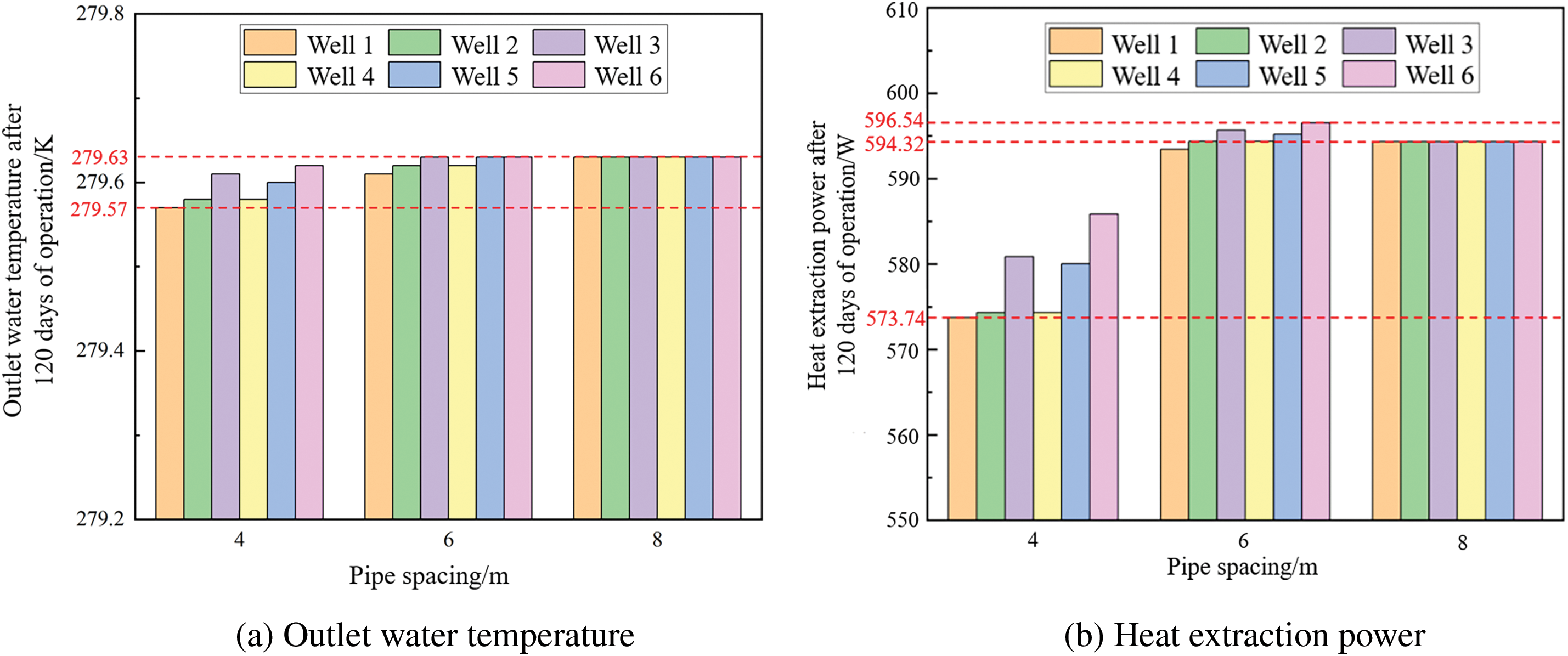
Figure 8: Thermal performance of different BHEs in the array under varying pipe spacings
Fig. 8a and b shows the BHE outlet temperature and heat extraction power at varying flow rates and pipe spacings. It can be observed that the differences among the various BHEs become more significant when the pipe spacing is smaller. When the borehole spacing is 4 m, the outlet water temperature of the BHEs located at the edge of the array is higher than that at the center, and their heat extraction power is also greater. As the BHE spacing increases to 6 and 8 m, the outlet water temperatures of the BHEs at different positions become nearly identical, and their heat extraction powers exhibit a similar trend. Compared to the outlet temperature, the differences in heat extraction power are more significant when the pipe spacing is smaller than 6 m. Additionally, the overall thermal performance of the BHEs decreases sharply as the pipe spacing decreases. When the BHE spacing changes from 4 to 6 m, the outlet water temperature rises, and the thermal performance improves significantly. However, as the spacing expands from 6 to 8 m, the outlet water temperature stabilizes around 279.63 K, and the heat extraction power stabilizes around 594.32 W. This occurs because, as the spacing increases, the thermal influence of each BHE on the others becomes negligible. Since the pump energy consumption is not considered, the differences in the BHE outlet temperatures are due to their positions and varying heat exchange rates. Moreover, when the flow rate escalates, the outlet water temperature shows a decreasing trend, fluctuating between 279.3 and 279.7 K. In contrast, the heat extraction power rises, ranging from 595 to 609 W.
This section investigates the variation trends of outlet water temperature and heat extraction power in the medium-deep BHE under different operating modes. The results for various conditions are illustrated in Figs. 9 to 11.
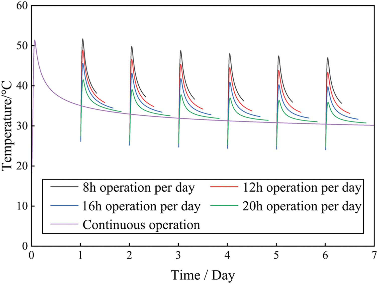
Figure 9: Variation of medium-deep BHE outlet water temperature under different daily operating times (7 days period)
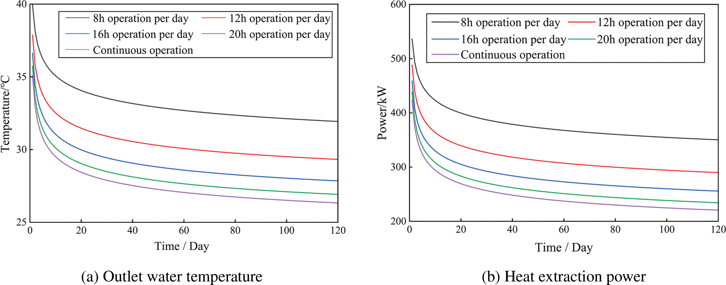
Figure 10: Thermal performance of a medium-deep BHE under different daily operating times (120 days)
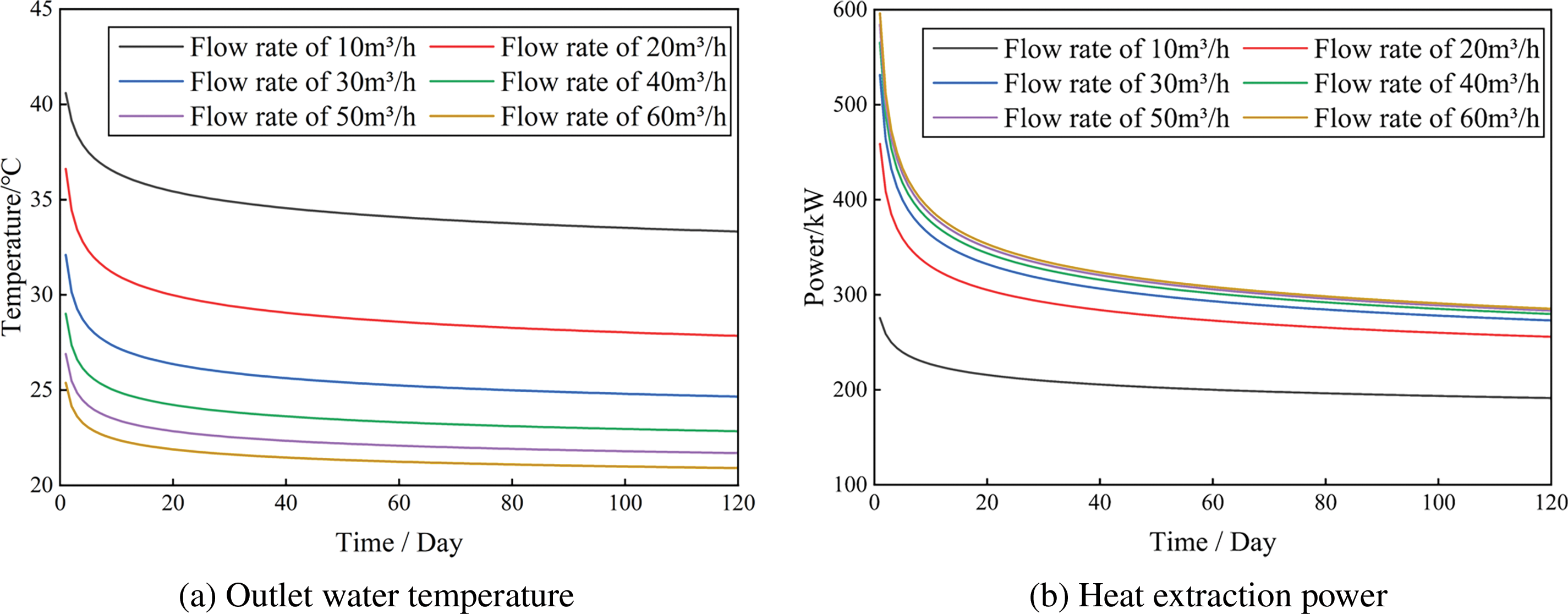
Figure 11: Thermal performance of a medium-deep BHE under different flow rates over 120 days
1) Medium-deep BHE performance affected by daily operating time
To facilitate observation, the variation curves of outlet water temperature over a 7-day operation of the BHE are summarized in Fig. 9. The outlet water temperature exhibits a pattern of fast escalation followed by a slow decline during each operational cycle (1 day). On the first day of operation, the curves for the same flow rate under different operating times overlap, indicating that the outlet water temperatures are identical for all cases. However, starting from the second day, differences in outlet water temperatures emerge as the daily operating time changes. Specifically, for conditions with longer operating durations, the outlet water temperature on the second day is lower. This is because the longer operating time allows the BHE to extract more thermal energy from the soil, while during non-operating periods, the ground temperature is not fully recovered. As the daily operating time increases, the differences in outlet water temperatures for different conditions become more significant.
The variation of BHE outlet water temperature over a 120-day heating season under different operating modes is then analyzed. For ease of observation, the outlet water temperatures recorded at the last time step of each day are selected as the representative temperature for each day. The curves illustrating the fluctuations in outlet water temperature and heat extraction power over 120 days across various operation modes are shown in Figs. 10a and b, respectively. The outlet water temperature demonstrates a consistently decreasing tendency under various scenarios. During the first ten days of operation, the temperature decreases rapidly, after which the rate of decline significantly slows down and gradually stabilizes. The larger the daily operating time, the lower the outlet water temperature becomes. Under an 8-h daily operation condition, the final outlet water temperature is 38°C, while continuous (24-h daily) operation results in a final outlet water temperature of only 31°C. This is because, with a constant flow rate, shorter operating times lead to less total heat extraction from the soil. During non-operational periods, the soil receives more heat from the surrounding geological formations and geothermal flow, allowing for more significant recovery of the soil temperature, which in turn ensures the stability of subsequent heat extraction and outlet water temperature. Additionally, throughout the 120-day operation period, the heat extraction power also shows a decreasing trend, with a gradually diminishing rate of decline. Conditions with longer daily operating times experience a faster reduction in heat extraction power. However, it is essential to recognize that reducing the daily operating hours may result in a decrease in total heat extraction. Therefore, it is necessary to reasonably design the daily operating time based on actual load requirements.
2) Medium-deep BHE performance affected by working fluid flow rate
Taking the 16-h daily operating time as an example, Fig. 11a and b illustrates the variation in outlet water temperature and heat extraction power over 120 days under different flow rates, respectively. Throughout the 120-day operational period, the outlet water temperature consistently demonstrates a declining tendency across all situations. There is a fast decrease in temperature during the first 5 days, after which the rate of decline significantly slows, and the outlet water temperature gradually stabilizes. The larger the flow rate, the lower the outlet water temperature. For a flow rate of 10 m3/h, the outlet water temperature at the end of the heating season is 34°C, while for a flow rate of 60 m3/h, the outlet water temperature drops to 21°C. This occurs because, with the same daily operating time, a higher flow rate results in a larger convective heat transfer coefficient, enabling the BHE to absorb more heat from the soil. However, the heat recovery during idle periods becomes insufficient. Additionally, over the 120-day operation period, the heat extraction power also shows a decreasing trend. There is a rapid decline in the first 10 days, followed by a significant slowdown in the rate of decline. The larger the flow rate, the higher the heat extraction power. For a flow rate of 10 m3/h, the final heat extraction power is 200 kW, while for a flow rate of 60 m3/h, the final heat extraction power reaches 300 kW.
In summary, the heat extraction power of the medium-deep BHE diminishes progressively with extended daily operational duration. A higher working fluid flow rate leads to greater heat extraction power. However, beyond a flow rate of 30 m3/h, additional increases have a minimal impact on the BHE’s heat extraction power. This flow rate is already close to the peak heat extraction power under ideal model conditions.
3.3 Comparison of Shallow and Medium-Deep BHE Systems
The results indicate that, in Xi’an, the stabilized heat extraction capacity of shallow BHEs varies from 595 to 609 W, contingent upon the pipe spacing. For the medium-deep BHE, under different operating modes and flow rates, the heat extraction power ranges from 200 to 400 kW. In practical applications, when there is sufficient space and simultaneous heating and cooling are required, tens to hundreds of shallow BHEs can be used. For buildings with a cooling load significantly larger than the heating load, medium-deep BHEs can be selected, as they occupy less area, or they can be combined with shallow BHEs.
4 Economic Efficiency Analysis
To further evaluate the economic viability of the two types of geothermal systems in practical applications, this section assesses the levelized cost of energy (LCOE) and the payback period (PBP) as key economic indicators.
1) Levelized Cost of Energy (LCOE)
The LCOE is determined by dividing the overall expenditures incurred throughout the project’s lifecycle by the total amount of energy produced over its lifespan. It represents the cost per unit of energy generated. This value accounts for factors such as time, the residual value of fixed assets, and depreciation of fixed assets. It can be calculated using the following formula [8]:
where the Pd is the construction cost, RMB. TO&M is the life cycle, year. Dd represents the asset depreciation rate, %. Rtax is the tax, %. Rd is the depreciation rate, %. PO&M is the operating costs, RMB. Vr is the residual value, RMB. Ea represents the annual heat extraction, kW.
2) Payback period (PBP)
In the BHE system project, the payback period (PBP) refers to the number of years required for the net present value of the project’s cash flows to equal zero, after discounting the annual net cash flows at a predetermined benchmark rate of return. This benchmark rate accounts for various factors, including inflation and depreciation. The PBP can be approximately determined by the duration required to recoup the initial investment expenditure [8].
For the shallow geothermal system, the average cost of obtaining thermal energy per kWh over its lifecycle (25 years) is investigated. The variations in LCOE across various operational situations are simulated and shown in Fig. 12a. It is evident that the LCOE decreases monotonically as the flow rate rises. Specifically, as the flow rate changes from 0.4 to 0.7 m/s, the LCOE drops from 0.70 to 0.54 RMB/kWh. Additionally, when the BHE spacing expands from 4 to 6 m, the LCOE decreases by approximately 1.59% to 2.06%. However, when the spacing expands from 6 to 8 m, there is no significant change in the LCOE. Fig. 12b shows that as the flow rate escalates, the PBP decreases from 11 to 10 years. Under constant flow conditions, the PBP for a borehole spacing of 6 m is lower than that for 4 m, with the maximum reduction across different flow rates ranging from 4.22% to 4.34%. The PBP for an 8 m spacing BHE array is slightly higher than that for a 6 m spacing. These results indicate that changes in PBP for shallow BHE systems are not significantly affected by medium flow rates or borehole spacing. The PBP is approximately two-fifths of the lifecycle.
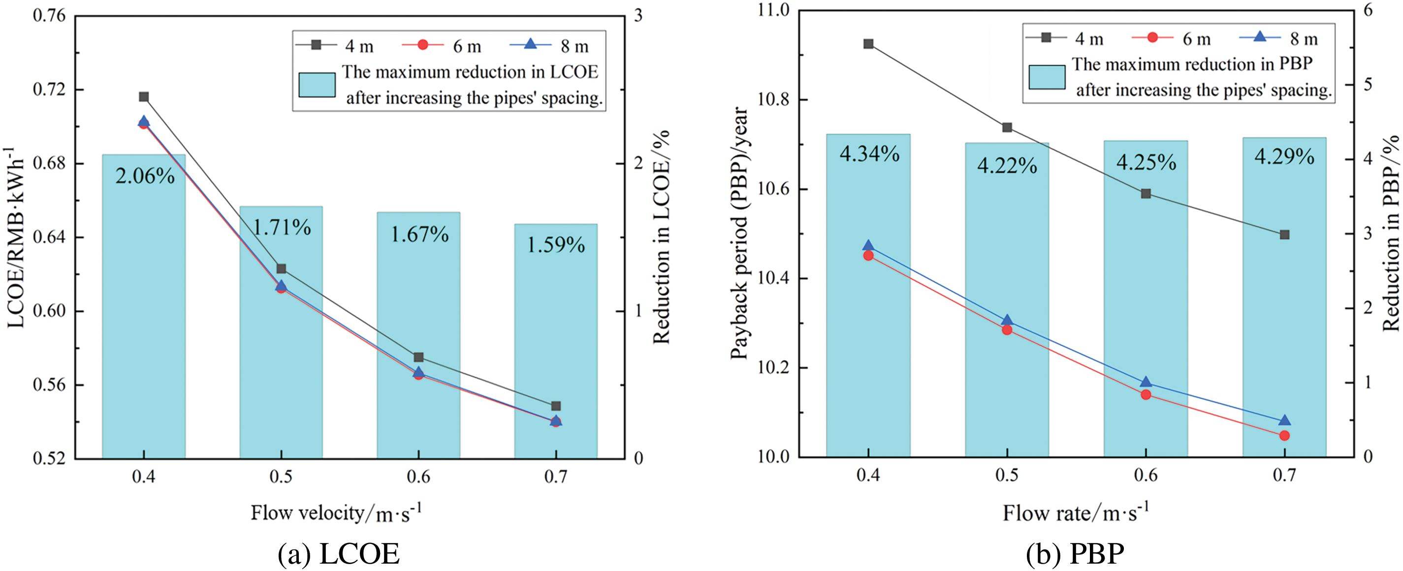
Figure 12: LCOE and PBP of shallow geothermal heating systems over 25 years of operation
Fig. 13 illustrates the trends in LCOE and PBP for a medium-deep geothermal system over 25 years. The yellow bars represent the maximum reduction in LCOE resulting from increased daily operating hours under different flow rates. From Fig. 13a, it can be observed that the LCOE initially decreases with increasing flow rate, reaches a minimum, and then rises again. Specifically, the LCOE is excessively high at flow rates of 10 and 60 m3/h. Within the range of 20 to 40 m3/h, the LCOE reaches lower values. When the flow rates is between 10 and 50 m3/h, larger daily operating hours result in a lower LCOE. This indicates that extending operating hours benefits the reduction of LCOE for medium-deep BHEs, particularly at smaller flow rates. For larger flow rates, the overall trend remains consistent. The flow rate corresponding to the minimum LCOE varies with different daily operating hour conditions. Notably, as daily operating hour increase, the flow rate that results in the minimum LCOE decreases. For instance, with 24 h of daily operation time, the flow rate corresponding to the minimum LCOE is 25 m3/h, with an LCOE value of 0.40 RMB/kWh. Thus, it is crucial to set operating hours and flow rates according to actual conditions to achieve the lowest LCOE.

Figure 13: LCOE and PBP of medium-deep geothermal heating systems over 25 years of operation
As shown in Fig. 13b, the PBP for other operating modes exceeds the lifecycle of the BHE (25 years), so only the results for 8- and 12-h daily operations are presented. The figure indicates that the PBP initially decreases and then increases with rising flow rates. At a constant flow rate, shorter daily operating hours lead to a smaller PBP, suggesting that extending operating hours is detrimental to reducing the system’s PBP. Specifically, when operating for 8 h a day, the minimum PBP can reach as low as 3 years, while for 12 h of daily operation, the minimum PBP is 12 years. Therefore, a well-considered design of flow rates and operating modes is essential to significantly reduce the PBP of the medium-deep BHE system.
4.3 Comparison of Shallow and Medium-Deep BHE Systems
A comprehensive comparison of the economic indicators for both systems reveals that the PBP for the shallow geothermal system typically ranges from 10 to 11 years. In contrast, the PBP for the medium-deep geothermal system shows a much wider variation, ranging from 3 to 25 years, with some conditions even exceeding the lifecycle (25 years). By adjusting system operating parameters, the LCOE for the shallow geothermal system can decrease by up to 22.86% (from 0.70 to 0.54 RMB/kWh). For the medium-deep geothermal system, the maximum reduction in LCOE can reach 52.94% (from 0.85 to 0.40 RMB/kWh). This indicates that the economic viability of the medium-deep geothermal heating system is more significantly influenced by operating parameters compared to the shallow system. Thus, through careful planning aligned with actual load requirements, there is considerable potential to significantly shorten the PBP of medium-deep BHE systems.
This study examines the thermal efficiency and economic viability of shallow and medium-deep geothermal heating systems. Based on geological parameters in the Xi’an region and typical borehole heat exchanger (BHE) structures, a comprehensive analysis is initially performed to examine the performance of shallow U-shaped BHEs under various spacing arrangements and operating parameters. The long-term performance and influencing factors of medium-deep coaxial BHEs are also analyzed. Finally, a comparative analysis of the economic aspects of the two systems is performed, intending to establish a theoretical foundation for the selection of heating systems and the optimization of their operational efficiency in actual applications. This study uses typical BHE systems, including a 50 m depth shallow BHE and a 2500 m depth medium-deep BHE, in Xi’an. The principal conclusions are as follows:
(1) For the shallow BHE system, increasing the BHE spacing reduces thermal interaction between boreholes. When the spacing increases to 6 m, the performance of the BHEs at different positions becomes independent of one another. With an increase in flow rate, the outlet water temperature ranges between 279.3 and 279.7 K, while the heat extraction power varies from 595 to 609 W.
(2) After 120 days of operation (the heating period in Northern China), the medium-deep coaxial BHE attains a heat extraction power of 245 kW when the system operates 8 h per day. In contrast, continuous operation (24 h a day) results in a heat extraction power of only 165 kW upon completion of the process. Moreover, the heat extraction power escalates with larger working fluid flow rates. However, once the flow rate exceeds 30 m3/h, further increases have a minimal influence on the heat extraction power. At this flow rate, the heat extraction power is close to the peak limit under ideal model conditions.
(3) The Levelized cost of energy (LCOE) for the medium-deep BHE system reaches a minimum value of 0.40 RMB/kWh. For the shallow BHE system, the LCOE decreases from 0.70 to 0.54 RMB/kWh as the flow rate increases. Moreover, the payback period (PBP) for the shallow system diminishes from 11 years to 10 years with increasing flow rates. In contrast, the PBP for the medium-deep system exhibits a more pronounced variation, ranging from 3 to 25 years. Thus, there is a greater potential for economic optimization in the medium-deep geothermal systems compared to the shallow systems. The findings offer theoretical insights for the assessment and optimal design of BHE systems.
(4) Considering both thermal performance and economic results, it is recommended to use shallow BHEs for buildings with both heating and cooling demands. The occupied area will be much larger than for medium-deep BHEs with the same heating load, but they can also be used in summer, and the PBP is relatively stable (10 to 11 years). For buildings with a greater emphasis on heating load, medium-deep BHEs are more appropriate because they occupy much less area. However, the PBP is highly sensitive to operating parameters. Thus, the optimal design of medium-deep BHEs is more critical.
Acknowledgement: Not applicable.
Funding Statement: The authors are grateful for the support by the Shanghai Engineering Research Center for Shallow Geothermal Energy (DRZX-202306), Shaanxi Coal Geology Group Co., Ltd. (SMDZ-ZD2024–23), Key Laboratory of Coal Resources Exploration and Comprehensive Utilization, Ministry of Natural Resources, China (ZP2020–1), Shaanxi Investment Group Co., Ltd. (SIGC2023-KY-05), Key Research and Development Projects of Shaanxi Province (2023-GHZD-54), Shaanxi Qinchuangyuan Scientist + Engineer Team Construction Project (2022KXJ-049) and China Postdoctoral Science Foundation (2023M742802, 2024T170721).
Author Contributions: Yuze Xue: Writing, Original draft, Conceptualization. Li Kou: Methodology, Investigation. Guosheng Jia: Data curation, Visualization, Supervision. Liwen Jin: Supervision, Methodology. Zhibin Zhang: Visualization, Writing. Jianke Hao: Data curation, Writing. Lip Huat Saw: Writing—review & editing, Validation. All authors reviewed the results and approved the final version of the manuscript.
Availability of Data and Materials: Not applicable.
Ethics Approval: Not applicable.
Conflicts of Interest: The authors declare no conflicts of interest to report regarding the present study.
References
1. Kitsopoulou A, Zacharis A, Ziozas N, Bellos E, Iliadis P, Lampropoulos I, et al. Dynamic energy analysis of different heat pump heating systems exploiting renewable energy sources. Sustainability. 2023;15(14):11054. doi:10.3390/su151411054. [Google Scholar] [CrossRef]
2. Koltunov M, Pezzutto S, Bisello A, Lettner G, Hiesl A, van Sark W, et al. Mapping of energy communities in Europe: status quo and review of existing classifications. Sustainability. 2023;15(10):8201. doi:10.3390/su15108201. [Google Scholar] [CrossRef]
3. Shamoushaki M, Koh SL. Comparative life cycle assessment of integrated renewable energy-based power systems. Sci Total Environ. 2024;946:174239. doi:10.1016/j.scitotenv.2024.174239. [Google Scholar] [PubMed] [CrossRef]
4. Wang T, Xiao D, Wu K, Zhu Q, Chen Z. Heat extraction evaluation of series/parallel U-shaped wells in middle-deep geothermal exploitation. Sustain Energy Technol Assess. 2025;73:104098. doi:10.1016/j.seta.2024.104098. [Google Scholar] [CrossRef]
5. Jia GS, Ma ZD, Xia ZH, Zhang YP, Xue YZ, Chai JC, et al. A finite-volume method for full-scale simulations of coaxial borehole heat exchangers with different structural parameters, geological and operating conditions. Renew Energy. 2022;182(1):296–313. doi:10.1016/j.renene.2021.10.017. [Google Scholar] [CrossRef]
6. Kurevija T, Macenić M, Tuschl M. Drilling deeper in shallow geoexchange heat pump systems—thermogeological, energy and hydraulic benefits and restraints. Energies. 2023;16(18):6577. doi:10.3390/en16186577. [Google Scholar] [CrossRef]
7. Wang X, Zhan T, Liu G, Ni L. A field test of medium-depth geothermal heat pump system for heating in severely cold region. Case Stud Therm Eng. 2023;48(4):103125. doi:10.1016/j.csite.2023.103125. [Google Scholar] [CrossRef]
8. Xia ZH, Jia GS, Tao ZY, Jia W, Shi YS, Jin LW. Multi-objective optimization of geothermal heating systems based on thermal economy and environmental impact evaluation. Renew Energy. 2024;237(6):121858. doi:10.1016/j.renene.2024.121858. [Google Scholar] [CrossRef]
9. Stober I, Bucher K. Geothermal energy: from theoretical models to exploration and development. Germany, Springer-Verlag Berlin Heidelberg: Springer; 2021. [Google Scholar]
10. Qi D, Pu L, Sun F, Li Y. Numerical investigation on thermal performance of ground heat exchangers using phase change materials as grout for ground source heat pump system. Appl Therm Eng. 2016;106(4):1023–32. doi:10.1016/j.applthermaleng.2016.06.048. [Google Scholar] [CrossRef]
11. Dai LH, Shang Y, Li XL, Li SF. Analysis on the transient heat transfer process inside and outside the borehole for a vertical U-tube ground heat exchanger under short-term heat storage. Renew Energy. 2016;87(3):1121–9. doi:10.1016/j.renene.2015.08.034. [Google Scholar] [CrossRef]
12. He Y, Jia M, Li X, Yang Z, Song R. Performance analysis of coaxial heat exchanger and heat-carrier fluid in medium-deep geothermal energy development. Renew Energy. 2021;168(1):938–59. doi:10.1016/j.renene.2020.12.109. [Google Scholar] [CrossRef]
13. Miocic JM, Schleichert L, Van de Ven A, Koenigsdorff R. Fast calculation of the technical shallow geothermal energy potential of large areas with a steady-state solution of the finite line source. Geothermics. 2024;116:102851. doi:10.1016/j.geothermics.2023.102851. [Google Scholar] [CrossRef]
14. Tang FJ, Nowamooz H. Factors influencing the performance of shallow Borehole heat exchanger. Energy Convers Manag. 2019;18(1):571–83. doi:10.1016/j.enconman.2018.12.044. [Google Scholar] [CrossRef]
15. Deng J, Wei Q, He S, Liang M, Zhang H. Simulation analysis on the heat performance of deep borehole heat exchangers in medium-depth geothermal heat pump systems. Energies. 2020;13(3):754. doi:10.3390/en13030754. [Google Scholar] [CrossRef]
16. Huang S, Li JQ, Zhu k, Dong JK, Jia YQ. Thermal recovery characteristics of rock and soil around medium and deep U-type borehole heat exchanger. Appl Therm Eng. 2023;224(2):120071. doi:10.1016/j.applthermaleng.2023.120071. [Google Scholar] [CrossRef]
17. Ingersoll LR. Theory of the ground pipe heat source for the heat pump. Heat Pip Air Condition. 1948;20:119–22. [Google Scholar]
18. Maghrabie HM, Abdeltwab MM, Tawfik MHM. Ground-source heat pumps (GSHPsmaterials, models, applications, and sustainability. Energy Build. 2023;299:113560. doi:10.1016/j.enbuild.2023.113560. [Google Scholar] [CrossRef]
19. Claesson J, Eskilson P. Conductive heat extraction to a deep borehole: thermal analyses and dimensioning rules. Energy. 1988;13(6):509–27. doi:10.1016/0360-5442(88)90005-9. [Google Scholar] [CrossRef]
20. Yu MZ, Lu W, Zhang FF, Zhang WK, Cui P, Fang ZH. A novel model and heat extraction capacity of mid-deep buried U-bend pipe ground heat exchangers. Energy Build. 2021;235:110723. doi:10.1016/j.enbuild.2021.110723. [Google Scholar] [CrossRef]
21. Hecht MJ, De PM, Beck M, Bayer P. Optimization of energy extraction for vertical closed-loop geothermal systems considering groundwater flow. Energy Convers Manag. 2013;66:1–10. doi:10.1016/j.enconman.2012.09.019. [Google Scholar] [CrossRef]
22. Gordon D, Bolisetti T, Ting K, Reitsma S. Short-term fluid temperature variations in either a coaxial or U-tube borehole heat exchanger. Geothermics. 2017;67:29–39. doi:10.1016/j.geothermics.2016.12.001. [Google Scholar] [CrossRef]
23. Mahariq I, Giden IH, Alboon S, Aly WHF, Youssef A, Kurt H. Investigation and analysis of acoustojets by spectral element method. Mathematics. 2022;10(17):3145. doi:10.3390/math10173145. [Google Scholar] [CrossRef]
24. Lu Q, Narsilio GA, Aditya GR, Johnston IW. Economic analysis of vertical ground source heat pump systems in Melbourne. Energy. 2017;125:107–17. doi:10.1016/j.energy.2017.02.082. [Google Scholar] [CrossRef]
25. Buonomano A, Calise F, Palombo A, Vicidomini M. Energy and economic analysis of geothermal-solar trigeneration systems: a case study for a hotel building in Ischia. Appl Energy. 2015;2015(138):224–41. doi:10.1016/j.apenergy.2014.10.076. [Google Scholar] [CrossRef]
26. Blum P, Campillo G, Kölbel T. Techno-economic and spatial analysis of vertical ground source heat pump systems in Germany. Energy. 2011;36(5):3002–11. doi:10.1016/j.energy.2011.02.044. [Google Scholar] [CrossRef]
27. Daniilidis A, Alpsoy B, Herber R. Impact of technical and economic uncertainties on the economic performance of a deep geothermal heat system. Renew Energy. 2017;114:805–16. doi:10.1016/j.renene.2017.07.090. [Google Scholar] [CrossRef]
28. Xia ZH, Jia GS, Ma ZD, Wang JW, Zhang YP, Jin LW. Analysis of economy, thermal efficiency and environmental impact of geothermal heating system based on life cycle assessments. Appl Energy. 2021;303(113):117671. doi:10.1016/j.apenergy.2021.117671. [Google Scholar] [CrossRef]
29. Erol S, Hashemi MA, François B. Analytical solution of discontinuous heat extraction for sustainability and recovery aspects of borehole heat exchangers. Int J Therm Sci. 2015;88(1–2):47–58. doi:10.1016/j.ijthermalsci.2014.09.007. [Google Scholar] [CrossRef]
30. Bu XB, Ran YM, Zhang DD. Experimental and simulation studies of geothermal single well for building heating. Renew Energy. 2024;143(5):1902–9. doi:10.1016/j.renene.2019.06.005. [Google Scholar] [CrossRef]
31. Zhang ZB, Ma ZD, Hao JK, Jia GS, Ke TT, Cheng CH, et al. Long-term operation performance of medium-deep borehole heat exchangers in the Guanzhong area. Coal Geol Explor. 2024;52(1):129–39 (In Chinese). doi:10.12363/issn.1001-1986.23.10.0706. [Google Scholar] [CrossRef]
Cite This Article
 Copyright © 2025 The Author(s). Published by Tech Science Press.
This work is licensed under a Creative Commons Attribution 4.0 International License , which permits unrestricted use, distribution, and reproduction in any medium, provided the original work is properly cited.
 Downloads
 Citation Tools