Research on the Optimal Scheduling Model of Energy Storage Plant Based on Edge Computing and Improved Whale Optimization Algorithm

Nomenclature

1  Introduction

As the electricity market booms, energy internet technologies continue to innovate. Management systems for large-scale energy storage plants are increasingly recognized as a key way to enhance the performance of multiple energy sources. It is also seen as a significant means of optimizing the synergistic operation of energy systems [1]. This topic has attracted significant attention and has become a focal point of research in energy systems domestically and internationally [2].

Current research on energy storage power plant management systems primarily focuses on key areas such as planning, operation, and optimal scheduling. Among these, optimal scheduling, which directly affects the operating costs of the system, has become a critical issue for energy storage plant management systems. Liu et al. [3] proposed a two-stage scheduling method combining day-ahead scheduling and real-time scheduling and designed an improved particle swarm optimization algorithm (IPSO) as the solution algorithm. Tostado-Véliz et al. [4] proposed a three-tier energy communities operation strategy that uses information gap decision theory (IGDT) to address the uncertainty of renewable energy generation and consumption. Li et al. [5] introduced a dynamic partitioning strategy to optimize the operation of centralized shared energy storage plants. However, in practical applications, this algorithm may fall short of meeting real-time operational and reliability requirements. Ali et al. [6] examined the impact of user demand and approached the economic dispatch problem of power systems from a fresh perspective. Yu et al. [7] employed an enhanced backpropagation algorithm to predict load growth, constructing an optimization model to minimize operation and maintenance costs. While these studies predominantly emphasize the economic aspects of coordinated planning for distributed power generation and energy storage, they overlook the influence of renewable energy uncertainty on optimizing energy system operations.

Kavousi-Fard et al. [8] proposed an advanced model for dynamic network reconstruction and optimal energy scheduling, utilizing mixed integer linear programming (MILP) techniques. Li et al. [9] proposed a two-phase methodology for planning distributed generation and energy storage systems, leveraging the principles of edge computing. This method specifically accounts for the hierarchical characteristics of energy storage loads. Liu et al. [10] conceptualized energy devices as multifunctional units and incorporated prediction error and penalty mechanisms to refine the renewable energy model. Tostado-VéLiz et al. [11] developed an innovative home energy management (HEM) tool, analyzing the impact of flexible loads and onboard batteries. The studies mentioned above primarily focus on energy storage system planning from a technical performance perspective.

To solve the problem of insufficient grid-connected renewable energy consumption capacity, Zhang et al. [12] proposed an adaptive improved genetic algorithm, which avoids falling into the local optimum. By integrating photovoltaics, diesel generators, and batteries into smart microgrids [13], they developed cost-effective electrification strategies that address the challenges of powering remote areas. The researchers introduced the distributed consensus alternating direction method of multipliers (ADMM) algorithm, which enhances the convergence speed and robustness of both smart grids and energy internet [14,15]. Zhou et al. [16] proposed a two-layer optimization design scheme for distributed power grids, focusing on optimizing load-side demand. Li et al. [17] developed a joint programming model, demonstrating the effectiveness of distributed computing through the particle swarm chaos optimization algorithm. Sun et al. [18] improved the firefly algorithm and achieved optimized scheduling of wind-solar complementary power generation systems. Qiu et al. [19] constructs a coordinated dispatch model based on two-stage distribution robust optimization, which integrates the collaborative relationship between electricity, heat and natural gas networks, and focuses on the analysis of economic operation and carbon emission issues. Though distributed computing is crucial to the economic dispatch process of energy storage systems, it also introduces additional costs related to energy equipment network transmission.

The decentralization of distributed power systems significantly increases the computational burden of managing the distribution network as a unified whole. Edge computing emerges as a practical approach [20], partitioning distributed generation into smaller subnets to enable more streamlined regional grid management. Each distributed device is enhanced with advanced communication capabilities, laying the groundwork for effective distributed computing. Nonetheless, challenges persist regarding the performance of data processing and network transmission. Moreover, there is a pressing need to optimize network transmission architecture, storage models, and solution algorithms to boost the efficiency of solar power generation and energy storage systems. In light of these challenges, this paper makes several key contributions, as outlined below:

1. Currently, centralized processing remains a prevalent approach within power system dispatch control. However, to fully explore the advantages of distributed processing, this study introduces edge computing to energy storage power plants and designs a novel edge computing architecture. By shifting most data processing and storage tasks to the network edge, this architecture achieves the decentralization of computing functions. As a result, it significantly reduces network transmission costs and offers a fresh perspective on the scheduling and control of energy storage power stations.

2. This article introduces an optimized scheduling model for energy storage plants, integrating demand response into its framework. It evaluates the economic efficiency of peak shaving, valley filling models, and collaborative energy storage systems through comprehensive numerical simulations. The results provide meaningful insights into optimizing the economic operation of energy storage power plants.

3. This paper compares four optimization algorithms: Genetic Algorithm (GA), Particle Swarm Optimization (PSO), Whale Optimization Algorithm (WOA), and the Improved Whale Optimization Algorithm (IWOA). GA excels in global search capability and is effective for optimizing multi-peak functions, but it suffers from slow convergence and is sensitive to parameter settings. PSO is simple and converges quickly, but it tends to become trapped in suboptimal solutions. Additionally, its performance is heavily dependent on the chosen parameters. In contrast, the IWOA is better suited for the complex scheduling challenges faced by energy storage plants, as it dynamically adjusts its strategy to enhance search accuracy and convergence speed. These algorithms are unconstrained optimization techniques, making them suitable for energy storage plant scheduling models.

2  Energy Storage Plant Management System Based on Edge Computing

2.1 Energy Information Exchange Optimization Model

For energy storage power plants with complex operating conditions and large amounts of scheduling data, adopting centralized optimization scheduling will face problems such as high energy consumption, high costs, and network transmission delays in scheduling operations. Edge computing technology can solve these problems by analyzing and processing the nearby data and transmitting the results to the cloud service application layer for unified scheduling. Based on this, the basic structure of the energy information exchange optimization model established for energy storage power plants is shown in Fig. 1.

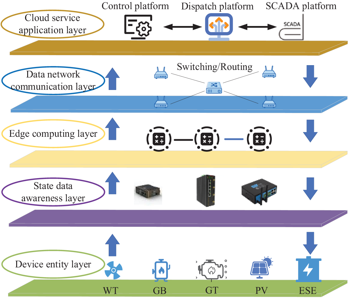
Figure 1: Basic structure of energy information exchange optimization model

The device entity layer concludes five devices: wind turbine (WT), gas boiler (GB), gas turbine (GT), photovoltaic (PV), and energy storage equipment (ESE). ESE includes three types of devices: electricity storage, heat storage, and gas storage. The main task of the device entity layer is to utilize various energy devices to generate electricity, heat, gas, and other energy sources to supply users and adjust the operating status of energy devices.

The state data sensing layer encompasses diverse intelligent modules for collecting and measuring energy data, primarily responsible for assisting the edge computing layer and cloud service application layer in monitoring the operational status of various energy devices.

The edge computing layer comprises modules dedicated to edge computing. These modules are mainly responsible for devising optimal operational strategies for diverse energy devices in the regional energy system. Their tasks include calculating the most efficient output levels and energy supply plans for these devices.

The data network communication layer consists of components such as data routers and wireless modules. Its primary function is to enable the efficient transfer of energy-related and scheduling data across layers, ensuring rapid and seamless data flow.

The cloud service application layer functions as the energy management hub, consisting of a Control platform, dispatch centers, and a Supervisory Control and Data Acquisition platform (SCADA) platform. The cloud service application layer optimizes energy supply solutions through computation and analysis, achieving improved efficiency in power exchange and distribution.

2.2 Edge Computing Architecture Design

Assume that the system architecture of the energy storage plant given in Fig. 1 contains e base station at the edge computing layer and u energy demand users. The base station at the edge computing layer is responsible for performing the edge computing tasks as well as realizing the data interaction with the data network communication layer. The set of edge computing layer base stations is denoted as E={1,2,⋯,e}, the set of energy demand users is denoted as U={1,2,⋯,u}, and all energy-demanding users satisfy the constraints of Eq. (1).

U=⋃kUk∈E(1)

where: U represents an energy consumption user set, E represents the union of a series of edge computing layer base station sets, k is taken from base station set E.

The base station within the edge computing layer offers robust data support and computational scheduling services to energy demand users and the cloud service layer. This functionality is enabled by the efficient integration of various components, such as edge computing modules, storage units, communication systems, and routing devices. Additionally, it can transmit collected and processed data to neighboring base stations in the edge computing layer, enabling collaborative operations across multiple stations. When the computational workload of a base station is minimal, it can independently handle the current scheduling task. The process of scheduling calculations for the energy storage plant based on edge computing is shown in Fig. 2.

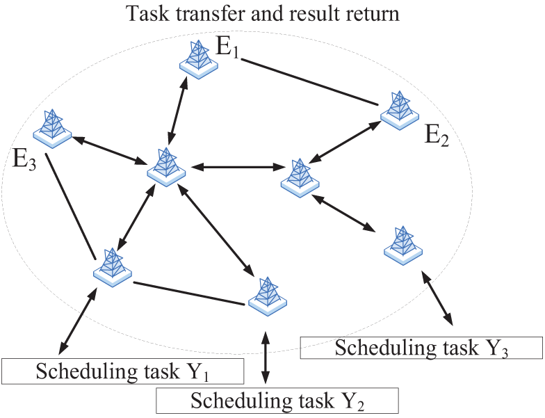
Figure 2: Schematic diagram of scheduling calculation process based on edge computing

When scheduling for an energy storage power plant, it is assumed that all energy devices and users with energy demands participate simultaneously in the system’s optimization process. Under this assumption, the computational task assignments for all edge computing layer base stations adhere to Eq. (2) to execute the scheduling process efficiently.

{S={xu,i,e}Su,i,e={1,useru′scomputational task iis assigned to base station e0,else(2)

where: S represents the set of system scheduling task assignment decisions, and Su,i,e is a specific value in the decision set S.

Furthermore, all computational tasks must be performed by at least one edge computing layer base station, a constraint given by Eq. (3).

{∑e∈Exu,i,e=1,∀u∈U,i∈YuRS,ecul=∑u∈U∑i∈Yucu,ixu,i,e≤Rmaxecul,e∈ERS,esto=∑u∈U∑i∈Yueu,ixu,i,e≤Rmaxesto,e∈E(3)

where: The first constraint guarantees that each computational task is handled by at least one base station. The second constraint imposes a limitation on the computational capacity of the base station, while the third pertains to the response performance related to the base station’s data storage capacity. RS,ecul, RS,esto are the responses of the computational and data storage capacities, respectively, with Rmaxecul, Rmaxesto denoting their upper limits. cu,i represents the computational requirements of the scheduling task, while su,i represents the data storage requirements of the scheduling task, and Yu refers to the optimized scheduling task within the system.

During the execution of optimized scheduling computation tasks, each task incurs energy consumption in both computation and data communication processes, accompanied by a certain transmission delay. The costs and transmission delays associated with the edge computing layer in performing these optimized scheduling computation tasks are outlined in Eq. (4).

{ Ccoop=NumECcul,eT¯coop=1Num∑u∈UTcoop,iTcoop,i−maxi∈Yu{Tu,isend+Tu,icul+Tu,imerge}+Tu,ireturn(4)

where: Ccoop represents the cost incurred for executing the optimal scheduling computation task. NumE denotes the number of base stations in the edge computing layer engaged in the task. Ccul,e refers to the operational cost of the equipment in the edge computing layer. Tcoop,i signifies the transmission delay while executing the optimized scheduling computation task, and T¯coop represents its average delay. Additionally, NumU indicates the total count of energy demand users. Tu,isend, Tu,icul, Tu,imerge, Tu,ireturn correspond to the delays in task dispatch, computation, result merging, and result return, respectively.

3  Optimized Scheduling Model for Energy Storage Plant Management System

3.1 Demand Response Model

Demand response (DR) refers to users adjusting their energy consumption behavior based on electricity price, participating in grid interactions, optimizing load curves, and improving system operational efficiency. Different types of loads exhibit varying degrees of sensitivity to identical electricity price signals. DR loads are categorized into two groups: curtailable loads (CL) and shiftable loads (SL). The following sections separately model these two load types.

3.1.1 CL characteristic Analysis and Modeling

CL determines whether to decrease its load by evaluating the variation in electricity price before and after the DR period. The characteristics of DR can be represented by a price-demand elasticity matrix. The element e(t,j) located at row t and column j of the elasticity matrix E(t,j), which represents the elasticity coefficient of the load at time t to the electricity price at time j, is shown in Eq. (5).

et,j=ΔPL,te/PL,te0Δρj/ρj0(5)

where: ΔPL,te represents the load variation at time t following DR; PL,te0 denotes the initial load at time t; Δρj indicates the variation of electricity price at time j after DR; ρj0 refers to the initial electricity price at time j.

The CL change ΔPCL,te at time t after DR is shown in Eq. (6).

ΔPCL,te=PCL,te0[∑j=124ECL(t,j)ρj−ρj0ρj0](6)

where: PCL,te0 represents the initial load that can be reduced at time t; ECL(t,j) is the price-demand elasticity matrix for CL; ρj denotes the electricity price at time j; and ρj0 indicates the initial electricity price at time j.

3.1.2 SL Characteristic Analysis and Modeling

SL refers to the load that users can adjust by modifying their working hours in response to electricity price, depending on their specific requirements. The transferable load change ΔPSL,te at time t after DR is represented in Eq. (7).

ΔPSL,te=PSL,te0[∑j=124ESL(t,j)ρj−ρj0ρj0](7)

where: PSL,te0 represents the initial transferable load at time t; ESL(t,j) denotes the price-demand elasticity matrix of SL.

3.2 Objective Function

The energy storage plant system considers DR to ensure that the system operates in compliance with various constraints while optimizing the overall economic efficiency of the entire network. The objective function is shown in Eq. (8), in order to minimize the sum of total electricity purchase cost CBuy and operation cost COP.

minF=CBuy+COP(8)

Electricity purchase cost CBuy is shown in Eq. (9). The energy storage plant engages in electricity trading with the higher-level power grid. When the generated electricity is insufficient to fulfill its demand, it buys additional power from the grid. Conversely, when there is an excess of generated electricity, the plant sells the surplus back to the higher-level grid.

CBuy=∑t=124(Pb,etκb,et−Ps,etκs,et+Qbtκgt)(9)

where: Pb,et and Ps,et are the power bought and sold from the higher-level electricity supplier at time t, respectively; κb,et and κs,et are the price of buying and selling electricity at time t, respectively; Qbt represents the purchase of natural gas at time t; κgt is the unit cost of natural gas.

Operation cost COp is shown in Eq. (10).

COp=∑t=124∑k=15wkPk,t(10)

where: k takes from 1 to 5, representing PV, GT, GB, WT and ESE, respectively, wk denotes the maintenance coefficient of the device k; Pk,t represents the output of the device k.

3.3 Constraint Condition

(1) The constraints for electric energy, gas energy, and heat energy are shown in Eq. (11).

{∑I1PI1,e(t)−Pein(t)+Peout(t)=PLe(t)∑I2PI2,g(t)−Pgin(t)+Pgout(t)=PLg(t)PGB,h(t)−Phin(t)+Phout(t)=PLh(t)(11)

where: PLe(t), PLh(t), PLg(t) are electric, heat and gas loads in the energy storage plant; I1 is a collection of energy equipment related to electricity, including WT, PV, and ESE; I2 is a collection of energy equipment related to gas energy, including GT and GB; Pein, Peout, Pgin, Pgout, Phin, Phout represent the charge and discharge power of the electric storage device, gas storage device, and heat storage device.

(2) The operational constraints of various equipment are shown in Eq. (12).

{PWTmin≤PWT(t)≤PWTmaxPGBmin≤PGB(t)≤PGBmaxPGTmin≤PGT(t)≤PGTmaxPPVmin≤PPV(t)≤PPVmaxPESEmin≤PESE(t)≤PESEmax(12)

where: PWTmin, PWTmax, PGBmin, PGBmax, PGTmin and PGTmax represent the minimum and maximum output power values of WT, GB and GT. PPVmin, PPVmax, PESEmin and PESEmax correspond to the minimum and maximum output power values of PV, ESE.

(3) Charge and discharge power constraints of the energy storage plant are shown in Eq. (13).

{Eesp(t)=Eesp(t−1)+[ηinPespin−1ηoutPespout(t)]△tEesp(0)=20%Eespmax10%Eespmax≤Eesp(t)≤90%Eespmax0≤Pespin(t)≤Uin(t)Pespmax0≤Pespout(t)≤Uout(t)PespmaxUin(t)+Uout(t)≤1Uin(t)∈{0,1},Uout(t)∈{0,1}(13)

where: Eesp(t) denotes the amount of energy stored in the energy storage plant; ηin and ηout refer to the charging and discharging efficiencies of energy storage devices; Pespin(t) and Pespout(t) represent the charging and discharging power of energy storage plant; Eesp(0) is the initial stored energy of the energy storage plant; Uin(t) and Uout(t) are the charging and discharging status bits of the energy storage plant, with variables ranging from 0 to 1.

3.4 Solution Process

This paper addresses the problem of minimizing the power purchase and operational costs of an energy storage plant while adhering to various constraints. The objective function incorporates both energy purchase costs and operational costs, factoring in demand response. The model is subject to constraints related to electricity, heat, and gas energy balance, along with the output power limits of the energy storage devices. The problem is solved using the CPLEX solver on the MATLAB platform, with optimization and comparison performed using Genetic Algorithm (GA), Particle Swarm Optimization (PSO), Whale Optimization Algorithm (WOA), and the Improved Whale Optimization Algorithm (IWOA). The solution process is illustrated in Fig. 3.

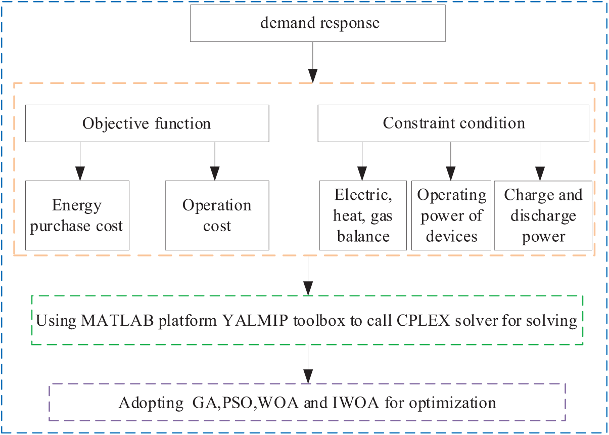
Figure 3: Solution flowchart

4  Algorithm for Solving Energy Optimization Scheduling Model

4.1 Whale Optimization Algorithm

Whales, due to their size, lack agility in the sea. To catch more small fish, they rely on unique cooperative methods to locate the largest fish group. They spiral upward and tighten their encirclement to reach the target fish group. WOA, inspired by their hunting, employs three position updating techniques: surrounding prey, rotation search, and random exploration.

4.1.1 Surrounding Prey

The whale communicates the information about the prey it has located and moves toward the closest whale within its group, progressively narrowing the encirclement to surround the prey. The formula for updating the whale’s position during this phase is shown in Eq. (14).

{Z(t+1)=Z∗(t)−A⋅DD=|C⋅Z∗(t)−Z(t)|(14)

where: t represents the number of search iterations, Z denotes the whale’s position; Z∗ refers to the global optimal position; A and C represent coefficient matrices, expressed as Eq. (15).

{A=2a⋅r1−aD=2r2a=2−2t/tmax(15)

where: r1 and r2 are randomly generated numbers within the interval [0, 1]; tmax represents the upper limit of iteration count; a is a linearly decreasing convergence factor, starting at 2 and ending at 0.

4.1.2 Rotation Search

Whales locate prey by spiraling upward and gradually closing in on the target. The equation for the spiral search is provided in Eq. (16).

{Z(t+1)=Z∗(t)+D⋅eblcos⁡(2πl)D=|C⋅Z∗(t)−Z(t)|(16)

where: b is a constant parameter that alters the spiral’s configuration; l is a randomly selected number from a uniform distribution within the range [−1, 1].

When whales search for prey in a spiral, they also contract their encirclement. Therefore, simulating this behavior requires both enclosing the prey and conducting a spiral search simultaneously. The updated formula is shown in Eq. (17).

Z(t+1)={Z∗(t)−A⋅|C⋅Z∗(t)−Z(t)|,p<0.5Z∗(t)+D⋅eblcos⁡(2πl),p≥0.5(17)

where: p represents a randomly generated number between [0, 1].

4.1.3 Random Exploration

To improve the whales’ global search capability and introduce a level of randomness in their prey-seeking behavior, the search area for the whale population is expanded.

When the coefficient |A| > = 1, it suggests that the whale is beyond the contracted enclosure and opts for a random search approach. Conversely, When the coefficient |A| < 1, it indicates that the whale is within the contracted encirclement and chooses the spiral encirclement search method. The formula for the random search update is provided in Eq. (18).

Z(t+1)=Zrand(t)−A⋅|C⋅Zrand(t)−Z(t)|(18)

where: Zrand is a random whale position.

The combination of the above three search methods constitutes the WOA.

4.2 Improved Whale Optimization Algorithm

Through analysis, it was found that WOA has limitations in terms of convergence speed and global search capability. Based on the standard whale position update method, three improvement strategies are introduced to form a global search strategy to enhance the algorithm’s optimization ability.

4.2.1 Adaptive Weight

Inspired by the PSO algorithm, we introduce a dynamic inertia weight w that changes according to the iteration count, influencing the position update of the whales. In the initial phases of the algorithm, the influence of the optimal whale’s position on the individual’s adjustment is diminished, thereby enhancing the global search ability during these initial phases.

As the iterations progresses, the effect of the optimal whale’s position grows, allowing other whales to converge more quickly towards it and thus speeding up the overall convergence of the algorithm. The adaptive inertia weight, chosen based on the change in update times in WOA, is given by Eq. (19).

w(t)=0.2cos⁡(π2⋅(1−t/tmax))(19)

where: The inertia weight w exhibits a non-linear behavior within the range [0, 1]. Due to the characteristics of the cosine function between [0, π/2], the weight starts small in the early algorithm phases, but the rate of change is quicker. In the later stages, the weight becomes larger, though its rate of change slows down, ensuring the algorithm’s convergence. The updated position formula for the IWOA is provided in Eqs. (20) and (21).

Z(t+1)={w(t)Z∗(t)−A⋅|C⋅Z∗(t)−Z(t)|,p<0.5w(t)Z∗(t)+D⋅eblcos⁡(2πl),p≥0.5(20)

Z(t+1)=w(t)Zrand(t)−A⋅|C⋅Zrand(t)−Z(t)|(21)

where: After introducing adaptive weights, the position update will dynamically adjust the weight size based on the increasing iteration count. This allows the optimal whale position Z∗(t) to offer different levels of guidance to individual whales at each point in the search. As the iterations progress, the whale group will gradually converge toward the optimal position. At this stage, a larger weight will enhance the movement of the whale positions, thereby speeding up the algorithm’s convergence.

4.2.2 Spiral Position Update

When whales hunt for prey, they modify their movement distance with each position update based on the spiral path between their current position and the target. In the spiral search model, b is a constant that dictates the spiral’s shape. This parameter is set to a constant, and the speed is adjusted according to different spiral radians each time the position is updated. However, keeping b constant can cause the whale’s spiral movement to follow a predictable pattern, consistently approaching the target along the same spiral path. This predictability may result in the algorithm converging to a local optimum, reducing its global search capability.

To resolve this issue and allow whales to explore more diverse search paths for position updates, we introduce the concept of variable helix search. The parameter b is designed to vary with the number of iterations, enabling dynamic adjustment of the helix shape during the whale search process. As a result, this enhances the whale’s capacity to explore unexplored regions and improves the algorithm’s overall global search effectiveness. When combined with adaptive weights, the updated helix position formula is presented in Eq. (22).

{Z(t+1)=w(t)Z∗(t)+bD⋅elcos⁡(2πl)b=e5⋅cos⁡(π⋅(1−t/tmax))(22)

where: The parameter b is defined based on the mathematical model of the spiral line. Building upon the foundational spiral path model, the spiral’s configuration is dynamically modulated by incorporating the iteration count. As the iterations increase, the formulated parameter b transitions from a larger to a smaller value.

Initially, the whale employs a broader spiral pattern to seek the target, aiming to extensively explore potential global optima, thereby improving the algorithm’s capacity for global optima. Subsequently, in the algorithm’s later phases, the whale adopts a narrower spiral pattern for target pursuit, refining the optimization accuracy of the process.

4.2.3 Optimal Neighborhood Disturbance

During position updates, whales generally aim for the current best-known position as their destination for each iteration. However, the optimal position often remains static unless a superior one is discovered, leading to a limited number of updates. This results in reduced search efficiency and slower exploration of the solution space. To address this limitation, we introduce an optimal neighborhood perturbation approach. This approach involves performing a randomized search around the optimal position with the intention of uncovering a more advantageous global solution. By diversifying the search process, this strategy not only speeds up the algorithm’s convergence but also reduces the likelihood of premature convergence, ensuring that the algorithm explores the solution space more thoroughly and avoids getting trapped in suboptimal local optima.

The optimal position introduces random variations, expanding its search within the surrounding area. The formula for the neighborhood perturbation is presented in Eq. (23).

X~(t)={X∗(t)+0.5⋅R1⋅X∗(t),R2<0.5X∗(t),R2≥0.5(23)

where: R1 and R2 are random numbers uniformly selected from the range [0, 1]; X~(t) represents the newly generated position.

For the generated neighborhood positions, a greedy strategy is applied to decide whether to keep them, and the corresponding formula is as Eq. (24).

X∗(t)={X~(t),f(X~(t))<f(X∗(t))X∗(t),f(X~(t))≥f(X∗(t))(24)

where: f(x) represents the position adaptation value of x.

If the newly generated position provides a better solution than the previous one, it will replace the original as the new global optimum. If not, the current optimal position will remain unchanged.

The optimal scheduling model solution process flow based on IWOA is represented as Fig. 4.

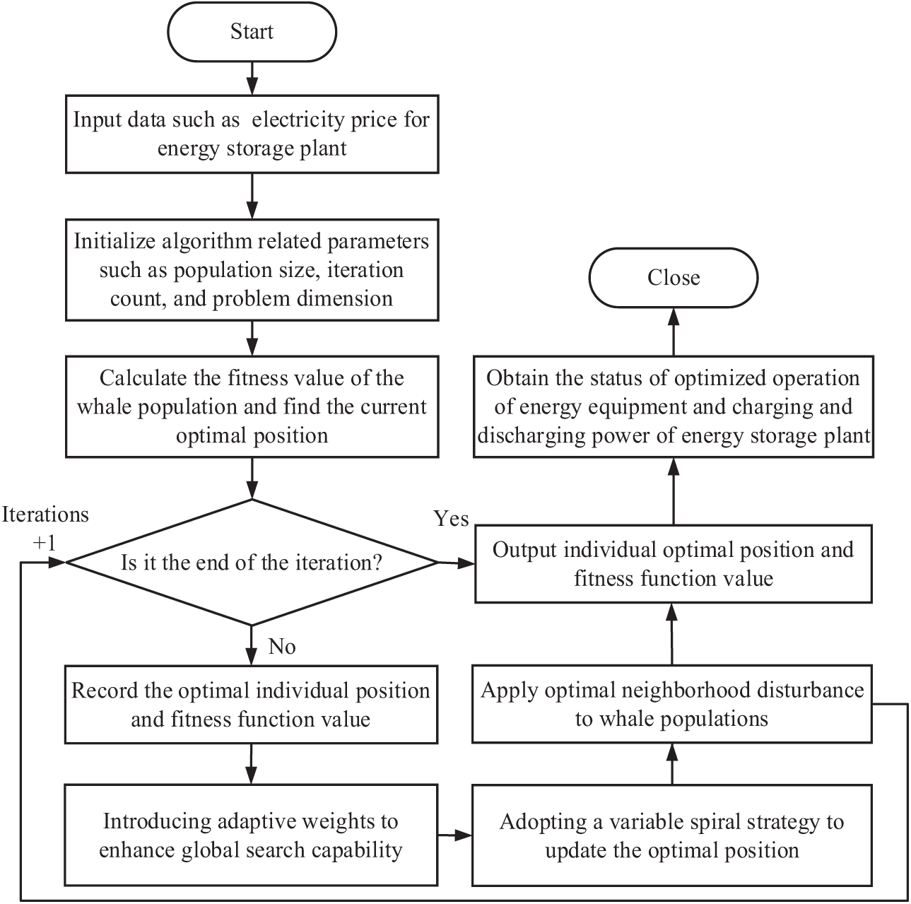
Figure 4: Optimal scheduling model solution process flow based on IWOA

The sensitivity analysis depicted in Fig. 5 focuses on evaluating the key parameters of network delay to identify those with the most significant impact on computational burden and system performance. By understanding these relationships, we can effectively target and optimize the most influential parameters. Given that the number of devices remains fixed, the analysis specifically targets network delay. In this setup, the sampling interval is configured to 1 h, while both the sampling delay and calculation delay are set at 0.2 h, providing a clear framework for optimizing the system’s performance under various conditions.

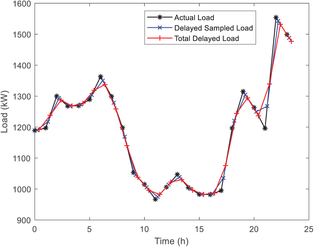
Figure 5: Delay analysis in sensitivity analysis

5  Calculation Results and Analysis

5.1 Example Setting

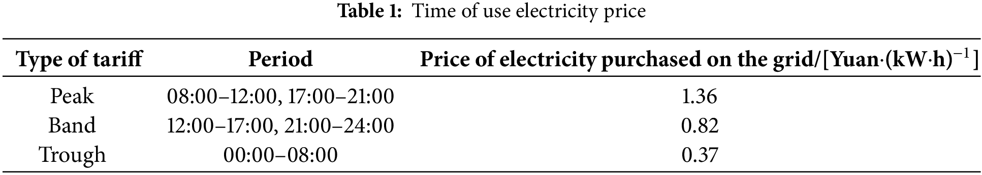
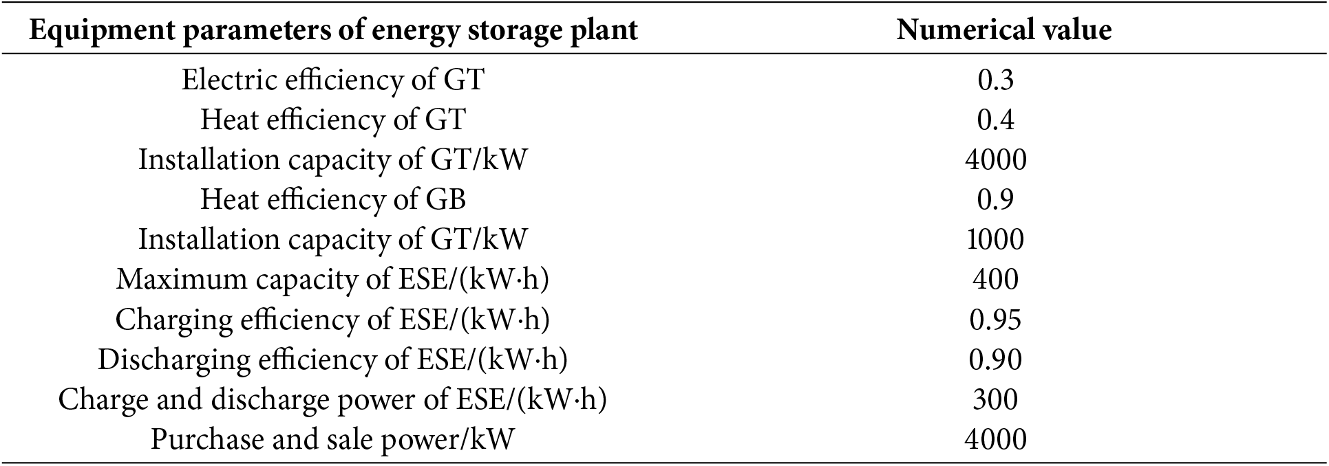
This paper takes an actual operating energy storage power station in Jiangsu Province as the research object and simulates its daily operation. The energy storage plant is mainly used for peak shaving and valley filling and assisting the stable operation of the power grid. In the study, it is assumed that the operation period is 24 h, the unit operation time is 1 h, and the operation of the power plant is modeled and analyzed with hourly granularity. The key equipment parameters are provided in Appendix A. The operation of the power plant involves the synergistic use of natural gas and electricity, with the natural gas’s price at 2.55 yuan/m3. The electricity rates under the time-of-day tariff strategy commonly applied in Jiangsu Province are presented in Table 1, which includes the peak, valley, and leveling periods.

5.2 Analysis of Optimization Scheduling Results for Energy Storage Plant

The energy optimization scheduling model proposed in this article minimizes the total cost of energy storage plant scheduling to obtain the optimal operating plan for each energy equipment. Figs. 5 and 6 are schematic diagrams of the electrical output power and heat output power of various equipment in the energy storage plant, respectively.

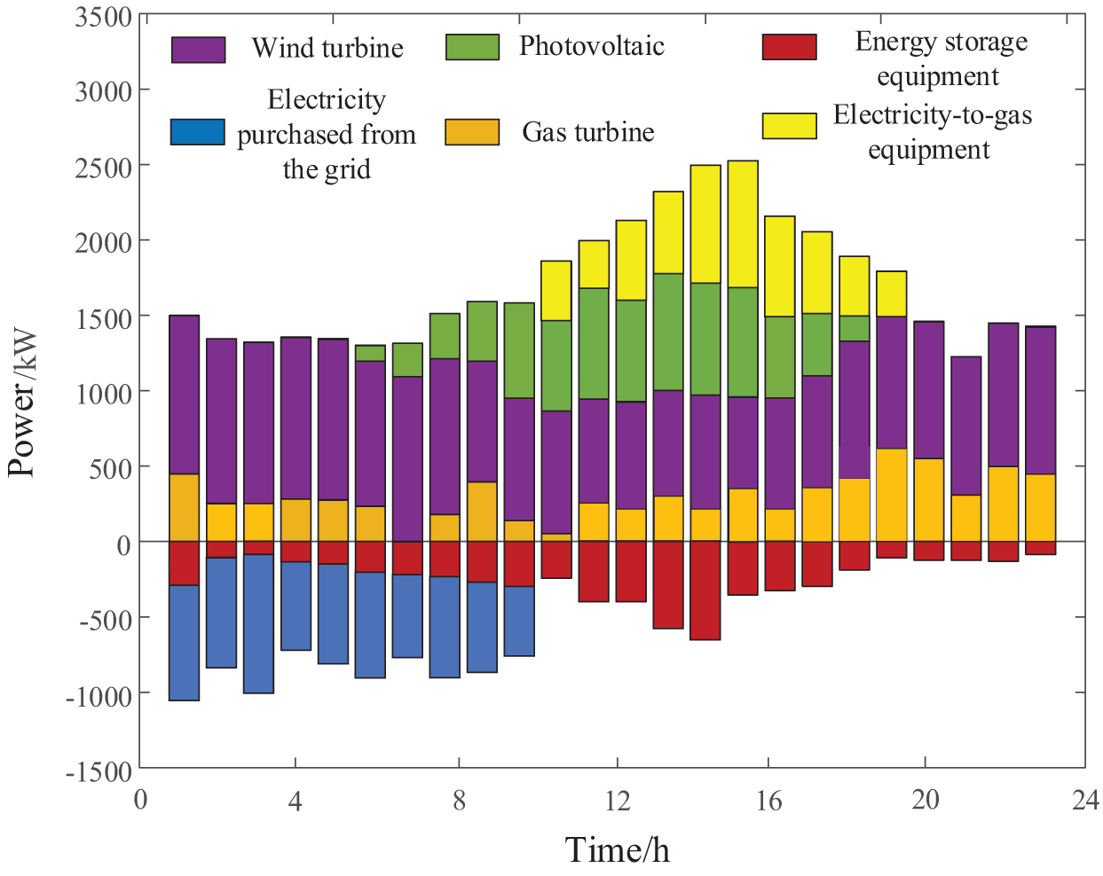
Figure 6: Electrical output power of each equipment

From the electrical power output of the device in Fig. 6, it is evident that the wind turbine’s output remains at a high level during all periods. The PV device outputs power to the energy storage station from 07:00–18:00, indicating the efficient utilization of renewable energy within the region. Other power generation units can flexibly adjust their output in response to fluctuations in load demand, ensuring that they can more accurately meet users’ load demands. When the price of electricity is low, energy storage plant tends to purchase more electricity from larger grids and charge energy storage devices. When the load demand increases, these storage devices release electricity to reduce operational and scheduling costs.

As shown in Fig. 7, the majority of the heat load is supplied by the gas turbine, with the gas boiler and heat-to-gas equipment serving as supplementary sources. From 00:00 to 07:00, the output of the gas boiler decreased the heat output of the gas turbine. This reduction in gas turbine output enables power dispatch to buy more electricity from the grid, while the excess power is stored in energy storage equipment, helping to lower operational costs during this period. From 10:00 to 15:00, the gas turbine runs at full load and the electricity load is also during peak hours. The comprehensive operation of the gas turbine can also make up for power shortages.

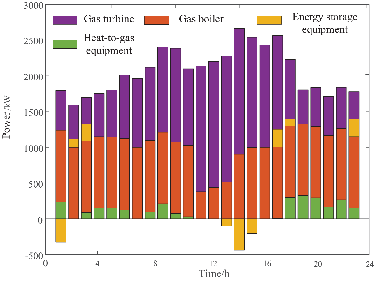
Figure 7: Heat output power of each equipment

From Figs. 8 and 9, compared with the original load distribution there is a significant difference between peaks and valleys, the high tariff period cuts part of the charge. Part of the load during the high tariff period is shifted to the low tariff period. This adjustment smooths the load curve. It reduces the load pressure during the high tariff period and increases the load utilization during the low tariff period. As a result, the goal of peak shaving and valley filling is effectively achieved.

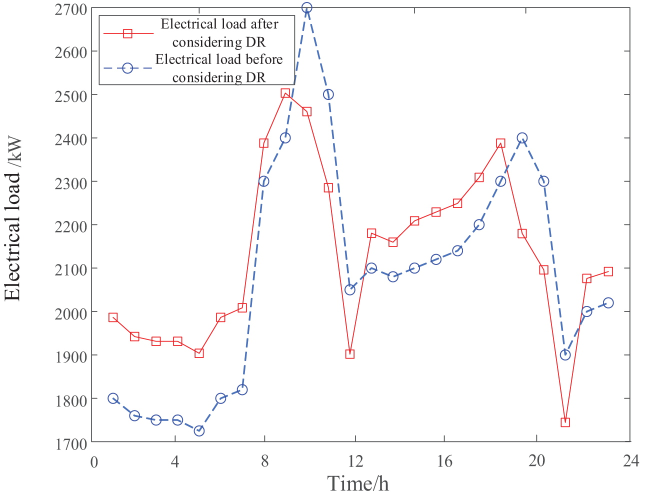
Figure 8: Comparison of electricity load before and after considering DR

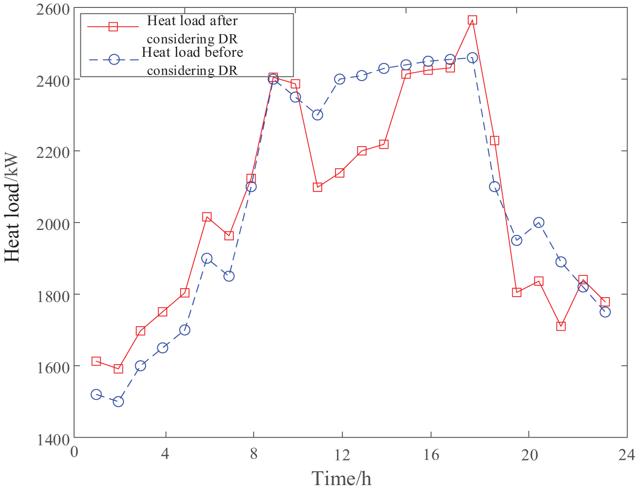
Figure 9: Comparison of heat load before and after considering DR

The electric load balance of the energy storage plant is illustrated in Fig. 10. A negative power value indicates that the energy storage plant is in the charging state, while a positive power value signifies discharging.

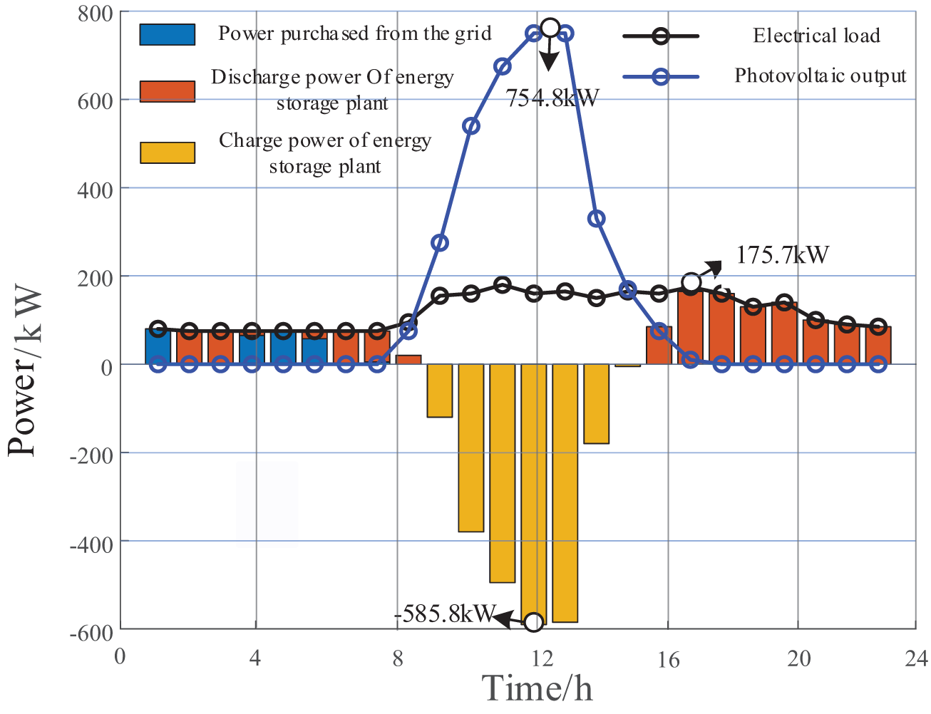
Figure 10: Electric load balance of energy storage plant

As shown in Fig. 10, from 00:00 to 08:30, the energy storage plant cannot meet its electricity load demand through PV power generation. To supplement electricity, its demand is met by discharging from energy storage equipment and buying electricity from the grid. From 08:30 to 15:00, the output of PV power generation exceeds the power load demand. The energy storage plant stores the excess electricity through energy storage equipment to avoid power waste. From 12:15 to 12:30, the output of PV reaches its maximum value of 754.8 kW, while the maximum charging power is 585.8 kW. From 15:00 to 24:00, PV output cannot meet the power load demand. This period also corresponds to the peak grid electricity price. To minimize operating costs, electricity is not bought from the grid. Instead, the energy storage plant releases energy to fulfill the load demand. From 16:30 to 16:45, the energy storage plant used energy storage equipment to release a maximum power of 175.7 kW.

By observing Fig. 11, during the periods 00:00–07:00 and 09:30–14:15, the energy storage plant is in the charging state. During the periods 08:00–09:30 and 14:15–24:00, the energy storage plant is mainly in the state of discharging. During the periods 11:45–12:00, the energy storage plant’s charging power reaches the maximum value of 635 kW, while during the periods 16:00–16:15, the energy storage plant’s discharging power hits its peak at 352 kW. From the above, it can be seen that the power demand of this steel plant has reached a state of equilibrium and there is no power abandonment. In addition, after one cycle of operation, the state of the energy storage plant returned to the initial stage, ensuring normal operation for the next cycle.

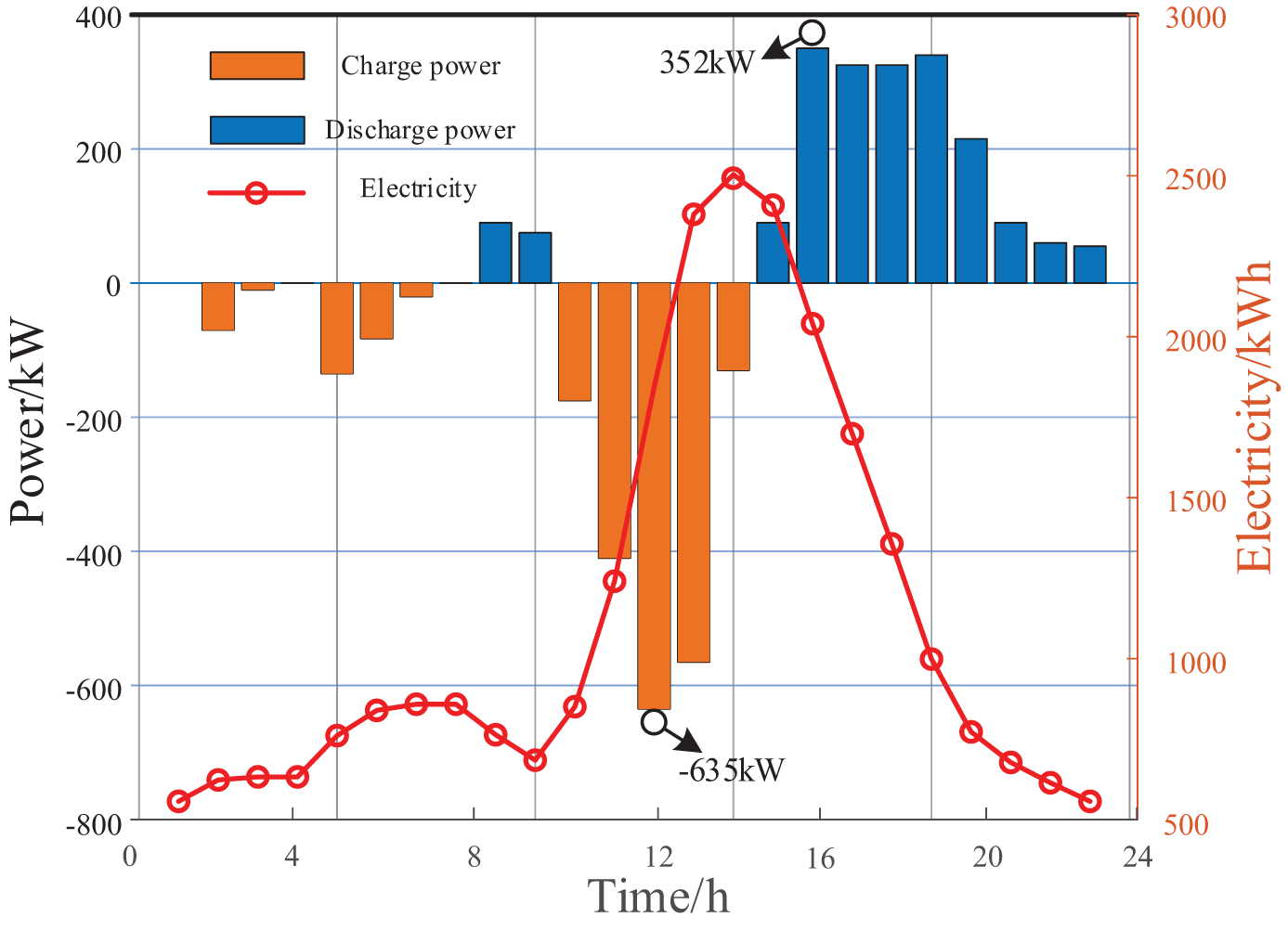
Figure 11: Charge and discharge power curves of energy storage plant

5.3 Comparative Analysis of Edge Computing Model and Centralized Scheduling Model

To verify the actual effectiveness of edge computing architecture, taking the number of regional power grids as 1, 5, and 10 as examples, the performance of traditional centralized scheduling strategy and edge computing scheduling strategy is compared by analyzing the network transmission time between energy devices and the number of iterations required to reach the same transmission time.

The data in Table 2 shows that as the number of regional power grids grows, the energy equipment data also increases accordingly, and the network transmission time for both scheduling strategies increases. However, compared with centralized scheduling, edge computing scheduling mode significantly reduces the network transmission time and transmission cost.

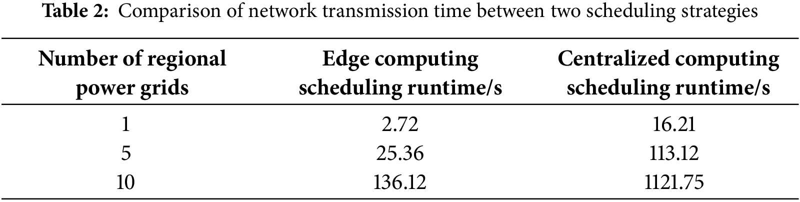
Table 3 shows the total number of iterations when comparing two strategies to achieve the same level of network transmission time between devices.

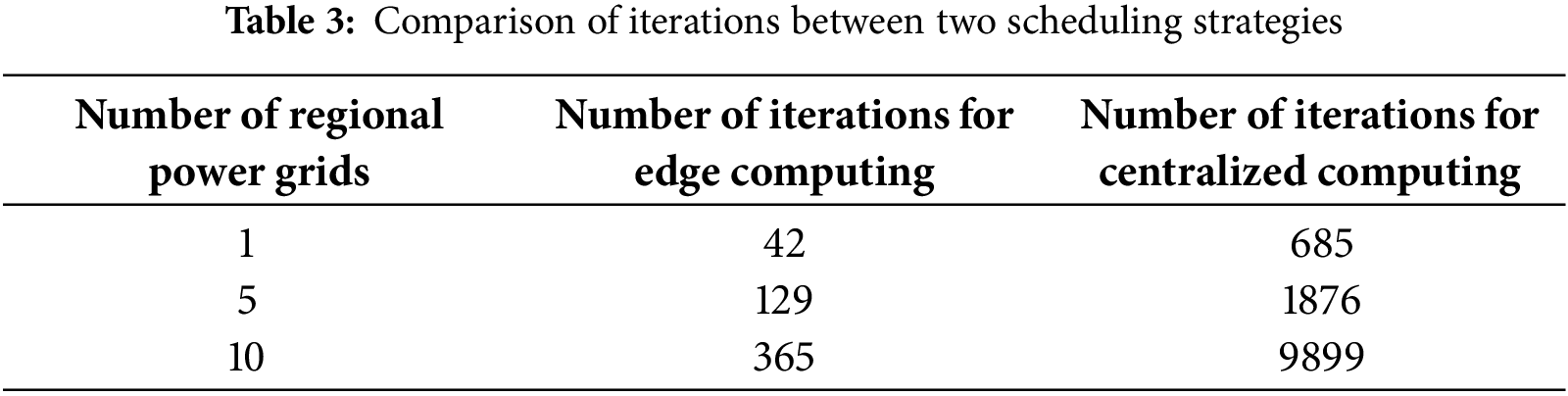
According to the comparison results in Table 3, since the edge computing architecture effectively allocates computing tasks to multiple edge nodes, the scheduling strategy under the edge computing architecture has significantly fewer iterations than the centralized scheduling strategy when achieving the same network transmission time. This result shows that the edge computing scheduling strategy has obvious advantages in reducing the number of iterations and improving computing efficiency.

5.4 Performance Analysis of Improved Whale Optimization Algorithm

To evaluate the performance of the IWOA, it was compared against GA, PSO, and WOA. For each algorithm, the benchmark test function was the combined total of the electricity purchase costs and operation costs, with a maximum iteration count set to 2000.

The results of solving the objective function are shown in Fig. 12. GA, PSO, and WOA have shown a tendency to converge to local optima. In contrast, IWOA enhances its global search ability through the variable spiral update method. This improvement enables the algorithm to overcome the limitations of local optima and identify new global optima. This indicates that the IWOA has higher optimization accuracy and lower scheduling costs.

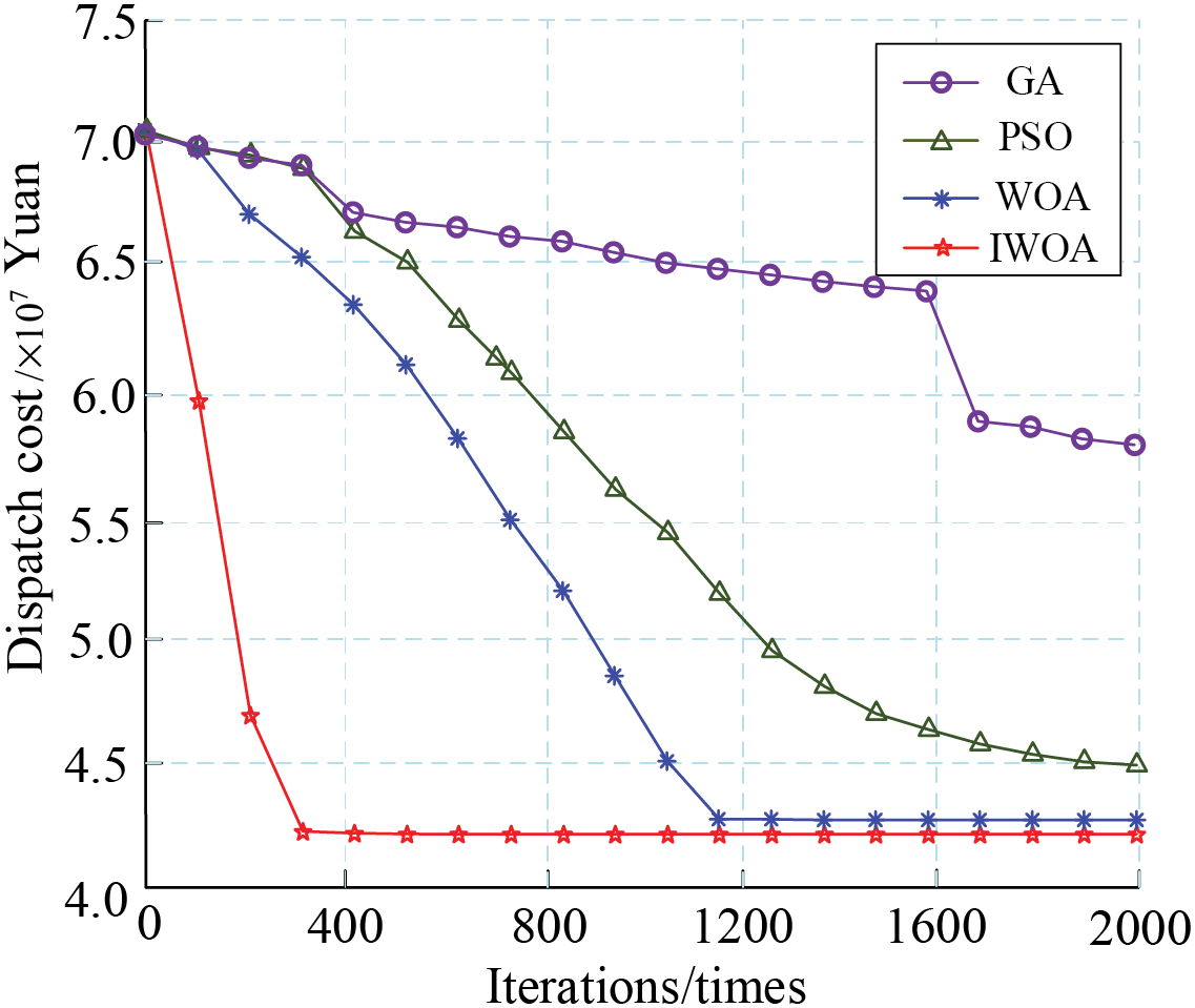
Figure 12: The results of each algorithm solving the objective function

6  Conclusion

To address the issues of high energy optimization costs and low energy utilization rates of energy storage equipment in energy storage power plants, this study proposes an optimal scheduling model based on edge computing and the improved whale optimization algorithm (IWOA). The model incorporates demand response and leverages edge computing architecture to minimize network transmission costs between energy devices. Additionally, it combines IWOA with an optimal neighborhood perturbation strategy to prevent the algorithm from becoming trapped in local optima. By analyzing the overall configuration of energy storage plants concerning demand response, the model’s economic viability and effectiveness are thoroughly evaluated. The case study analysis yields the following conclusions:

(1)   In contrast to the traditional centralized scheduling strategy, the proposed edge computing scheduling approach significantly reduces network transmission time between energy devices and the number of iterations required at the edge layer.

(2)   Compared to traditional algorithms, the IWOA excels in minimizing electricity purchase and operational costs.

(3)   The optimized scheduling model for energy storage plants, which incorporates demand response, has demonstrated the economic benefits of peak shaving, valley filling, and collaborative energy storage systems. This model provides valuable insights into the cost-effective operation of energy storage plants.

While our research has yielded promising results, it is important to recognize some limitations and identify areas for future exploration. Variations in parameter settings in IWOA can lead to widely varying results, which poses a challenge in generalizing the model across different energy storage device configurations. The integration of an edge computing layer introduces additional hardware and software requirements. Therefore, the cost, maintenance, and security of distributed computing nodes must be carefully evaluated to ensure cost-effectiveness and operational flexibility.

In our future work, we will explore the impact of the variability and security of edge computing on the system. Our goal is to enhance the robustness and performance of the scheduling model. Additionally, we will consider other critical factors, including environmental sustainability, the lifecycle impacts of energy storage technologies, and their long-term viability. In conclusion, while our current research has made significant strides in optimizing energy storage power plants, there remain several areas that require improvement and further exploration. This will help to fully leverage the potential of edge computing and advanced optimization algorithms in this field.

Acknowledgement: The authors would like to express their sincere gratitude to Jiangsu Key Laboratory of Power Transmission and Distribution Equipment Technology.

Funding Statement: This work was supported by the Changzhou Science and Technology Support Project (CE20235045), Open Subject of Jiangsu Province Key Laboratory of Power Transmission and Distribution (2021JSSPD12), Talent Projects of Jiangsu University of Technology (KYY20018) and Postgraduate Research & Practice Innovation Program of Jiangsu Province (SJCX23_1633).

Author Contributions: The authors acknowledge their respective roles in the paper as follows: study conception and design: Zhaoyu Zeng; data collection: Fuyin Ni; analysis and interpretation of results: Fuyin Ni; draft manuscript preparation: Zhaoyu Zeng. All authors reviewed the results and approved the final version of the manuscript.

Availability of Data and Materials: The data can be provided upon request.

Ethics Approval: Not applicable.

Conflicts of Interest: The authors declare no conflicts of interest to report regarding the present study.

Appendix A

References

1. Men XY, Cao J, Wang ZS. The constructing of multi-energy complementary system of energy internet microgrid and energy storage model analysis. Proc CSEE. 2018;38(19):5727–37. doi:10.13334/j.0258-8013.pcsee.172419. [Google Scholar] [CrossRef]

2. Ai Q, Hao R. Key technologies and challenges for multi-energy complementarity and optimization of integrated energy system. Automat Elect Power Syst. 2018;42(4):2–10+46. doi:10.7500/AEPS20170927008. [Google Scholar] [CrossRef]

3. Liu X, Xie S, Tian J, Wang P. Two-stage scheduling strategy for integrated energy systems considering renewable energy consumption. IEEE Access. 2022;10:83336–49. doi:10.1109/ACCESS.2022.3197154. [Google Scholar] [CrossRef]

4. Tostado-Véliz M, Mansouri SA, Rezaee-Jordehi A, Icaza-Alvarez D, Jurado F. Information Gap Decision Theory-based day-ahead scheduling of energy communities with collective hydrogen chain. Int J Hydrog Energy. 2023;48(20):7154–69. doi:10.1016/j.ijhydene.2022.11.183. [Google Scholar] [CrossRef]

5. Li J, Fang Z, Wang Q, Zhang M, Li Y, Zhang W. Optimal operation with dynamic partitioning strategy for centralized shared energy storage station with integration of large-scale renewable energy. J Mod Power Syst Clean Energy. 2024;12(2):359–70. doi:10.35833/MPCE.2023.000345. [Google Scholar] [CrossRef]

6. Ali M, Abdulgalil MA, Habiballah I, Khalid M. Optimal scheduling of isolated microgrids with hybrid renewables and energy storage systems considering demand response. IEEE Access. 2023;11:80266–73. doi:10.1109/ACCESS.2023.3296540. [Google Scholar] [CrossRef]

7. Yu X, Yang K. Distribution network optimization model of industrial park with distributed energy resources under the carbon neutral targets. Energy Eng. 2023;120(12):2741–60. doi:10.32604/ee.2023.028041. [Google Scholar] [CrossRef]

8. Kavousi-Fard A, Zare A, Khodaei A. Effective dynamic scheduling of reconfigurable microgrids. IEEE Trans Power Syst. 2018;33(5):5519–30. doi:10.1109/TPWRS.2018.2819942. [Google Scholar] [CrossRef]

9. Li J, Zhang Y, Chen C, Wang X, Shao Y, Zhu X, et al. Two-stage planning of distributed power supply and energy storage capacity considering hierarchical partition control of distribution network with source-load-storage. Energy Eng. 2024;121(9):2389–408. doi:10.32604/ee.2024.050239. [Google Scholar] [CrossRef]

10. Liu K, Liang C, Wu N, Dong X, Yu H. Energy economic dispatch for photovoltaic-storage via distributed event-triggered surplus algorithm. Energy Eng. 2024;121(9):2621–37. doi:10.32604/ee.2024.050001. [Google Scholar] [CrossRef]

11. Tostado-Véliz M, Hasanien HM, Turky RA, Rezaee Jordehi A, Mansouri SA, Jurado F. A fully robust home energy management model considering real time price and on-board vehicle batteries. J Energy Storage. 2023;72(1):108531. doi:10.1016/j.est.2023.108531. [Google Scholar] [CrossRef]

12. Zhang H, Tian Y. Coordinated optimal scheduling of WPHTNS power system based on adaptive improved genetic algorithm. IEEE Access. 2023;11:95600–15. doi:10.1109/ACCESS.2023.3309305. [Google Scholar] [CrossRef]

13. Mukundufite F, Bikorimana JMV, Lugatona AK. Smart micro grid energy system management based on optimum running cost for rural communities in Rwanda. Energy Eng. 2024;121(7):1805–21. doi:10.32604/ee.2024.051398. [Google Scholar] [CrossRef]

14. He X, Zhao Y, Huang T. Optimizing the dynamic economic dispatch problem by the distributed consensus-based ADMM approach. IEEE Trans Ind Inform. 2020;16(5):3210–21. doi:10.1109/TII.2019.2908450. [Google Scholar] [CrossRef]

15. Attarha A, Scott P, Thiébaux S. Affinely adjustable robust ADMM for residential DER coordination in distribution networks. IEEE Trans Smart Grid. 2020;11(2):1620–9. doi:10.1109/TSG.2019.2941235. [Google Scholar] [CrossRef]

16. Zhou S, Han Y, Chen S, Yang P, Mahmoud K, Darwish MMF, et al. A multiple uncertainty-based bi-level expansion planning paradigm for distribution networks complying with energy storage system functionalities. Energy. 2023;275:127511. doi:10.1016/j.energy.2023.127511. [Google Scholar] [CrossRef]

17. Li Y, Feng B, Wang B, Sun S. Joint planning of distributed generations and energy storage in active distribution networks: a Bi-Level programming approach. Energy. 2022;245(2):123226. doi:10.1016/j.energy.2022.123226. [Google Scholar] [CrossRef]

18. Sun L, Bao J, Pan N, Jia R, Yang J. Optimal scheduling of wind-photovoltaic-pumped storage joint complementary power generation system based on improved firefly algorithm. IEEE Access. 2024;12:70759–72. doi:10.1109/ACCESS.2024.3401756. [Google Scholar] [CrossRef]

19. Qiu Y, Li Q, Ai Y, Chen W, Benbouzid M, Liu S, et al. Two-stage distributionally robust optimization-based coordinated scheduling of integrated energy system with electricity-hydrogen hybrid energy storage. Prot Control Mod Power Syst. 2023;8(1):33. doi:10.1186/s41601-023-00308-8. [Google Scholar] [CrossRef]

20. Gu L, Zhang W, Wang Z, Zeng D, Jin H. Service management and energy scheduling toward low-carbon edge computing. IEEE Trans Sustain Comput. 2023;8(1):109–19. doi:10.1109/TSUSC.2022.3210564. [Google Scholar] [CrossRef]