SGP-GCN: A Spatial-Geological Perception Graph Convolutional Neural Network for Long-Term Petroleum Production Forecasting

1  Introduction

Accurate petroleum production forecasting is fundamental for effective oilfield management. It is essential not only for evaluating production capacity but also for providing a decision basis for reservoir engineers [1]. A reliable and scientifically grounded long-term production forecasting facilitates the rational organization of oilfield operations, ultimately helping to achieve strategic objectives. Therefore, accurate forecasting of long-term petroleum production is crucial for oilfields. However, petroleum production is affected by various factors, including geology, technology, and economics [2]. It often exhibits non-linear and non-stationary features, posing a significant challenge to achieving accurate long-term petroleum production forecasting.

Traditional methods for production forecasting in the petroleum industry include numerical simulation, water flooding characteristic curves, and statistical methods. Numerical simulation is currently the most widely employed technique for petroleum production forecasting in oilfields. However, its accuracy heavily depends on robust history matching and precise geological modeling, often requiring substantial computational resources [3,4]. Moreover, the requisite parameters are often unavailable in many cases. The water flooding characteristic curve is another prevalent forecasting method; however, when the water cut in an oilfield exceeds 90%, the curve tends to undergo upward warping, leading to significant forecasting errors [5,6]. Furthermore, statistical methods, which determine production by analyzing data, generally exhibit poor adaptability and computational accuracy [7].

The rapid development of artificial intelligence has provided new perspectives to revisit traditional and important problems in the petroleum industry [8]. Compared with traditional statistical methods, machine learning methods can automatically learn data features with higher accuracy and stronger generalization ability. Noshi et al. [9] used algorithms such as gradient boosting decision tree (GBDT) to screen production-sensitive features and used the support vector regression (SVR) model to forecast petroleum production. Ng et al. [10] utilized SVR and feed-forward neural networks (FNNs), integrated with particle swarm optimization (PSO), to forecast the well production in the Volve field. Although machine learning models generally perform well, they rely heavily on extensive manual data pre-processing and feature engineering, which makes it challenging to handle large-scale and high-dimensional data effectively [11].

In recent years, deep learning has gained significant traction in the field of petroleum production forecasting [12–14]. Recurrent neural networks (RNNs), known for their ability to extract and learn features layer by layer from raw data, have become a popular choice for this purpose [15]. Ibrahim et al. [16] applied RNNs to model and forecast the production sequences of oil, water, and gas. Due to the inability of fully connected neural networks (FCNNs) to directly store and utilize information from previous moments, Wang et al. [17] employed the long short-term memory network (LSTM) to forecast oil production during high water cut periods. Cheng et al. [18] analyzed the limitations of the Arps declining curve and combined LSTM with the gated recurrent unit network (GRU) for oil production forecasting. Additionally, some researchers have utilized machine learning algorithms to identify key factors influencing production prior to forecasting, thereby enhancing accuracy. Liu et al. [19] used the mean decrease impurity (MDI) algorithm to identify the primary factors and then applied LSTM for production forecasting. Conversely, Liu et al. [20] employed the XGBoost algorithm to screen the key factors of production and utilized a multivariate LSTM model to forecast production during high water cut periods.

The single RNNs have limitations in extracting potentially complex relationships within production data. Consequently, researchers have explored methods that integrate RNNs with convolutional neural networks (CNNs) to extract relevant features more effectively [21,22]. Zha et al. [23] proposed a CNN-LSTM model, which successfully merges the feature extraction capabilities of CNNs with the sequence prediction strengths of LSTM. Building on this, Pan et al. [24] introduced a CNN-LSTM-SA model incorporating the self-attention mechanism to capture correlations among petroleum production data, enhancing forecasting accuracy.

Those composite models often possess strong feature extraction and sequence forecasting capabilities; however, they typically focus on achieving great predictive performance for individual production wells. In the context of multiple production wells within the same study area, those models tend to overlook the selective utilization of valuable information from other wells, often struggling in the forecasting of long-term production that exhibits non-stationary features. During the development, there may be similar yet asynchronous processes of production changes among wells. Selectively integrating these information from other wells can help the production wells learn the long-term production change patterns that are relevant to the current well, thus improving the accuracy of long-term production forecasting.

In this study, we propose a spatial-geological perception graph convolutional neural network (SGP-GCN). We hypothesize that production wells with similar geological and spatial features are inherently more likely to exhibit analogous patterns of production change. To capture these relationships, we utilize geological feature correlations and spatial distances to construct a spatial-geological matrix. This enables SGP-GCN to perceive the geological and spatial information of production wells, allowing it to selectively utilize information transmitted from each well. Furthermore, petroleum production is not only influenced by inherent factors but external factors. To address this, we propose a matrix sparsification algorithm based on production clustering (SPC). By reducing attention on production wells with significant production discrepancies, this method optimizes weight distribution within the spatial-geological matrix, ultimately enhancing the forecasting accuracy of long-term petroleum production.

2  Related Technologies

2.1 Graph Convolutional Neural Network

Graph convolutional networks (GCNs) are a class of deep learning methods designed for graph-structured data, which have been widely applied to spatio-temporal sequence forecasting, such as infectious disease forecasting [25,26], crime forecasting [27] and traffic flow forecasting [28,29]. GCNs propagate information from neighboring nodes to the current node through convolution operations and aggregate the information to update the node state. This process is referred to as message passing. Through multiple layers of message passing, GCNs can capture information from multiple order neighbors. The message passing formulation of GCNs is defined as follows:

H(l+1)=σ(D−1AH(l)W(l)),(1)

where A is the adjacency matrix of the undirected graph with self-connections, D is the diagonal matrix that records the degree information of the undirected graph, Dii = ∑jAij, W(l) is the trainable weight matrix of the lth layer, σ(−) is the activation function, H(l) and H(l+1) ∈ ℝN×E are the node embeddings in the lth and l + 1th layers, respectively, N is the number of nodes, and E is the node embeddings dimension.

2.2 Multi-Scale Dilated Convolutional Network

Convolutional neural networks (CNNs) have exhibited remarkable feature extraction capabilities and efficient parallel processing performance on lattice and sequence data through learnable filters [30]. Some researchers have integrated multiple parallel convolutional layers with the same filters but varying step sizes and dilation rates into a multi-scale dilated convolutional network (MDCN) [31,32]. This approach aims to capture temporal dependencies at different granularities, enabling the extraction of multiple patterns from time series data. The multi-scale dilated convolution for one-dimensional data can be defined as:

ds[i]=∑z=1Lxs[i+k×z]×c[z],(2)

where ds is the output feature vector, xs is the raw feature vector, c is a convolution filter of length L, and k is the dilation rate. Specifically, we use a set of filters with different k and L to form the MDCN.

2.3 Self-Attention Mechanism

The self-attention mechanism (SA) is a feature extraction method designed to capture global correlations within data, first introduced by Vaswani et al. [33] in 2017. This mechanism generates query (Q), key (K), and value (V) vectors by linearly transforming the input features. A self-attention score is computed based on the similarity between the query and key vectors. The value vector is then weighted and summed to produce the final output. This approach enables the model to dynamically adjust the weights of different elements, thereby enhancing its ability to capture correlations within the features more effectively. The self-attention score α is calculated as:

α(Q,K)=softmax(QKTdk),(3)

where softmax(−) is the normalized exponential function and dk is the dimension of key vectors.

3  Spatial-Geological Perception Graph Convolutional Neural Network (SGP-GCN)

3.1 Feature Selection

During the development, a substantial amount of data related to production wells is accumulated. Based on the type and source of the data, it can be categorized into two main types:

•   Dynamic production data: This category includes variables such as oil production, water production, gas production, bottom-hole flow pressure, and water cut. It is derived from production records and monitoring data, reflecting the energy changes and production status of wells post-commissioning. It features a large number of samples and exhibits pronounced time series characteristics.

•   Static geological data: This includes variables such as permeability, porosity, and oil saturation. It originates from well logging data and represents the inherent characteristics of reservoirs, closely correlating with the reserves and production capacity of reservoirs.

Additionally, we selected the average geodetic coordinates of the production wells within each sub-layer to measure the spatial distances between them.

For the dynamic production data, the MDI feature selection method is employed to analyze the importance of each feature in relation to production. During this process, we eliminated redundant features with low importance and retained the remaining features as effective features of dynamic production data.

Related studies have indicated a significant correlation between geological features and production [34,35]. Among these, oil saturation and porosity are critical parameters for reserve estimation, while permeability, effective thickness, and formation pressure are essential components of Dupuit production formula, as represented in Eq. (4).

Q=2πKoh(Pe−Pw)μln⁡(ReRw),(4)

where Q is the oil production, Ko is the oil permeability, h is the effective thickness, Pe and Pw are the formation pressure and bottom-hole flow pressure, μ is the viscosity of the oil, and Re and Rw are the drainage radius and wellbore radius, respectively.

Consequently, oil saturation, porosity, permeability, effective thickness, and formation pressure are identified as effective features of the static geological data. Due to the limited quantity of well logging records for each production well, we utilized geological features before production to characterize the geological relationships between the production wells and to identify those wells that are more likely to provide valuable information for production forecasting. The SGP-GCN model is constructed based on the data mentioned above, as illustrated in Fig. 1.

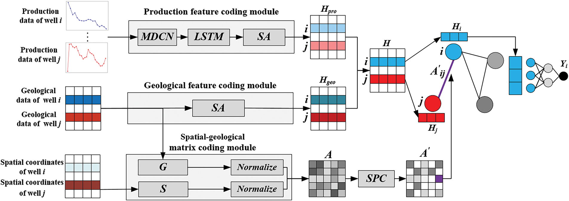
Figure 1: SGP-GCN model

3.2 Feature Coding

3.2.1 Production Feature Coding Module

For production well i, we define its sliced dynamic production data as Di,pro = [di,1, di,2, …, di,T] ∈ RE×T, where E represents the feature dimension and T represents the time step length. The features of Di,pro are extracted using MDCN to obtain the dynamic production features Xi,pro = [xi,1, xi,2, …, xi,T] ∈ RK×T. Assuming that K is the dimension of the LSTM hidden state, for each input element xi,t, LSTM performs the hidden state update as follows:

hi,t=tanh(wxi,t+Uhi,t−1+b),(5)

where hi,t and hi,t−1 are the hidden state of the LSTM at time t and t − 1, respectively, tanh(−) is the nonlinear activation function, U ∈ RK×K is the weight matrix, and w, b ∈ RK are the adaptive weights and biases vector, respectively.

The hidden state at the last moment hi,T is selected as the output of the LSTM. Subsequently, the internal correlations of the production features is captured by the self-attention layer to obtain the production feature encoding Hi,pro for production well i:

Hi,pro=αi,proVi,pro,(6)

where αi,pro is self-attention score of hi,T, Vi,pro is linearly transformed vectors generated from the hi,T.

3.2.2 Geological Feature Coding Module

In this module, we employ a self-attention layer to capture the internal correlations within Dgeo, which leads to the generation of the geological feature code Hgeo.

3.2.3 Spatial-Geological Matrix Coding Module

To construct the geological feature matrix G, we set Gij to represent the correlation between the static geological features of production well i and production well j, which is calculated as:

Gij=fatten(Di,geo)⋅fatten(Dj,geo)||fatten(Di,geo)||⋅||fatten(Dj,geo)||,(7)

where fatten(−) is the spreading function that spreads the static geological features from multi-dimensional to one-dimensional, and Di,geo and Dj,geo denote the static geological data of the production well i and production well j, respectively.

To construct the spatial distance matrix S, we set Sij to represent the proximity in spatial distance between the production well i and production well j, which is calculated as:

Sij={1(xi−xj)2+(yi−yj)2,i≠j0,i=j,(8)

where xi and xj represent the average horizontal coordinate of production well i and production well j in each sub-layer, respectively, and yi and yj are their average vertical coordinate.

After normalizing the matrix S and the matrix G, the corresponding elements are summed to obtain the spatial-geological matrix A:

Aij=(Sij−SminSmax−Smin)+(Gij−GminGmax−Gmin),(9)

where Smin and Smax are the minimum and maximum values of the matrix S, and Gmin and Gmax are the minimum and maximum values of the matrix G, respectively.

3.3 Matrix Sparsification Algorithm Based on Production Clustering (SPC)

In this study, we characterize the relationships between production wells based on spatial distance and geological feature correlations, constructing the spatial-geological matrix A as the weight matrix. During the message passing process, each production well assigns different attention weights to information received from other production wells according to matrix A.

However, petroleum production is influenced by inherent factors, such as geological features, as well as external factors, such as well stimulation [36]. A comparative analysis of production data indicates that certain production wells exhibit significant discrepancies in production rates and demonstrate lower correlations within the production data, despite having relatively high correlations in terms of spatial and geological features. Such variation suggests that these wells may be impacted by external factors that limit their effectiveness in improving forecasting accuracy. Within the initial spatial-geological matrix, information from these wells may still receive disproportionately high attention weights. We refer to this type of information that has deviated from its intended weight as “deviated information”, and we define the connections that convey such information as “deviated connections”.

To address this issue, we propose a matrix sparsification algorithm based on production clustering (SPC), which is designed to sparse the spatial-geological matrix by integrating production clustering with the attention mechanism. By utilizing the attention mechanism, we selectively eliminate connections between production wells that belong to different categories within the spatial-geological matrix. This method reduces the emphasis on production wells that exhibit substantial discrepancies in their production data, as the deviated information from these wells tends to exert a greater influence on forecasting accuracy. The specific steps of this process are outlined as follows:

•   Set a base threshold: Eliminate connections in matrix A with values below the base threshold, allowing production wells to prioritize information from other wells that exhibit stronger spatial and geological feature correlations.

•   Clustering using K-Means: Apply the K-Means clustering algorithm to the production data in the training set. To achieve optimal partitioning of production data, the silhouette coefficient is used as an evaluation metric to determine the optimal number of clusters.

•   Set an inter-class threshold: After clustering, compute the attention scores between the production data of each production well using Eq. (3) and sort them accordingly. Based on this, the inter-class threshold is set to remove connections between production wells belong to different categories that have lower attention scores, resulting in a sparsified spatial-geological matrix A′.

The SPC allows the SGP-GCN to concentrate more on information from production wells with similar production change processes during message passing, thereby reducing the negative impact of deviated information on production forecasting. This process is illustrated in Fig. 2.

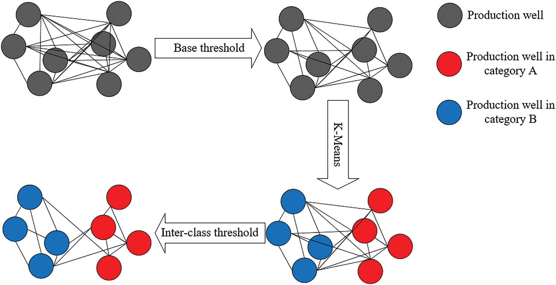
Figure 2: Matrix sparsification algorithm based on production clustering

3.4 Production Forecasting

For production well i, splice its production feature coding Hi,pro and geological feature coding Hi,geo to generate the spatio-temporal feature coding Hi as its representation:

Hi=[Hi,pro;Hi,geo].(10)

Normalize the matrix A′ while setting its diagonal elements to 1. With it as the adjacency matrix, while defining the diagonal matrix D whose diagonal element Dii is the sum of the elements of the ith row of matrix A′:

Dii=∑j=1NAij′,(11)

where N is the total number of production wells.

The message passing is performed through Eq. (1) and finally the production forecasting results are obtained using the fully connected layer.

The algorithm of SGP-GCN is shown in Algorithm 1:

4  Data and Training

4.1 Data Introduction

The data for this study come from an oilfield in Northern China, covering an area of approximately 15 square kilometers. The oilfield has been in development since June 1995. A substantial amount of monthly production data has been accumulated over this period. For this study, 50 oil production wells with complete observation records were selected. Their monthly average daily oil production data from December 1999 to December 2023, totaling 289 months, will serve as the dataset for the proposed experiment. As production proceeds, some of the production wells are converted to water injection wells.

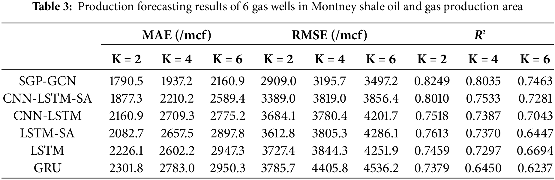
To further validate the effectiveness of the SGP-GCN model, we incorporated production data from multiple oil and gas fields. This includes production data from 6 gas wells located in the Montney shale oil and gas production area of Canada, covering a period of 110 months. The gas wells selected for this analysis are M3, M18, M23, M27, M1, and M24. For static geological data, four key metrics were utilized to assess the geological features of the wells: total organic carbon in weight per cent (TOC), amount of free hydrocarbons per gram of rock (S1), amounts of hydrocarbons generated through thermal cracking of non-volatile organic matter per gram of rock (S2) and amount of CO2 produced during the thermal breakdown of kerogen per gram of rock (S3).

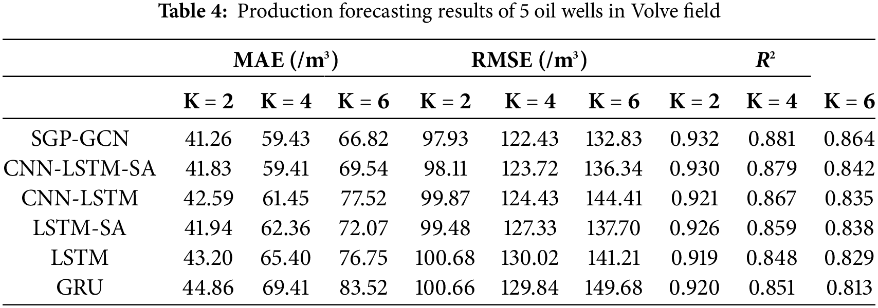
Additionally, we selected five production wells from the Volve oil field in southern coastal region of Norway: NO 15/9-F-1 C, NO 15/9-F-11 H, NO 15/9-F-12 H, NO 15/9-F-14 H, and NO 15/9-F-15 D. The production data for these wells spans 744 days, from 8 April 2014, to 21 April 2016. For the static geological data, we selected attributes such as Net/Gross, Total porosity, Total water saturation, and Horizontal permeability from the Heather, Hugin, and Sleipner formations, noting that geological data for the Sleipner formation is not available for wells NO 15/9-F-1 C and NO 15/9-F-11 H. In the experiments on those two datasets, the adjacency matrix was constructed from geological information only.

4.2 Data Pre-Processing

Due to the different units of various attributes for the same production well and the significant differences in their orders of magnitude, attributes with larger scales tend to dominate the model. This can negatively impact the accuracy and model training speed. To enhance forecasting accuracy and accelerate the model training speed, the data is standardized using a min-max normalization approach, as follows:

Z=X−XminXmax−Xmin,(12)

where X is the individual data observation, Xmin is the minimum value of the original data and Xmax is the maximum value of the original data.

4.3 Model Training

When training the SGP-GCN model with the normalized data, the dataset is divided into training, validation, and test sets in the proportions of 50%, 20%, and 30%, respectively. The window size is set to 20, with forecasting steps at 2, 4, and 6. During the training process, the model uses historical production data from the past 20 time steps to forecast future production at the 2nd, 4th, and 6th time steps, corresponding to short-term, medium-term, and long-term production forecasting, respectively.

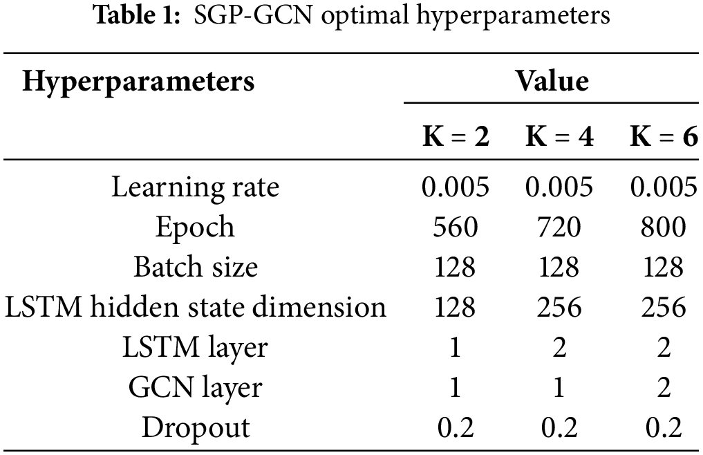
We employ four filters to construct the MDCN, with dilation rates and filter sizes of (1, 3), (1, 5), (2, 3), and (2, 5), respectively. In the training phase, a grid search method is employed to select the optimal hyperparameters, which are summarized in Table 1.

5  Results

5.1 Dynamic Production Feature Selection Result

The production data includes several attributes such as water production, bottom-hole flow pressure, and water cut in addition to oil production. The importance of the remaining attributes on oil production was calculated using the MDI feature selection method. The results are shown in Fig. 3, where cumulative oil production, cumulative liquid production, and cumulative water production have low importance on oil production, and their exclusion does not have a significant impact on the model accuracy. Therefore, connected well injection, monthly liquid production, bottom-hole flow pressure, monthly water production, and water cut are retained as effective features of dynamic production data.

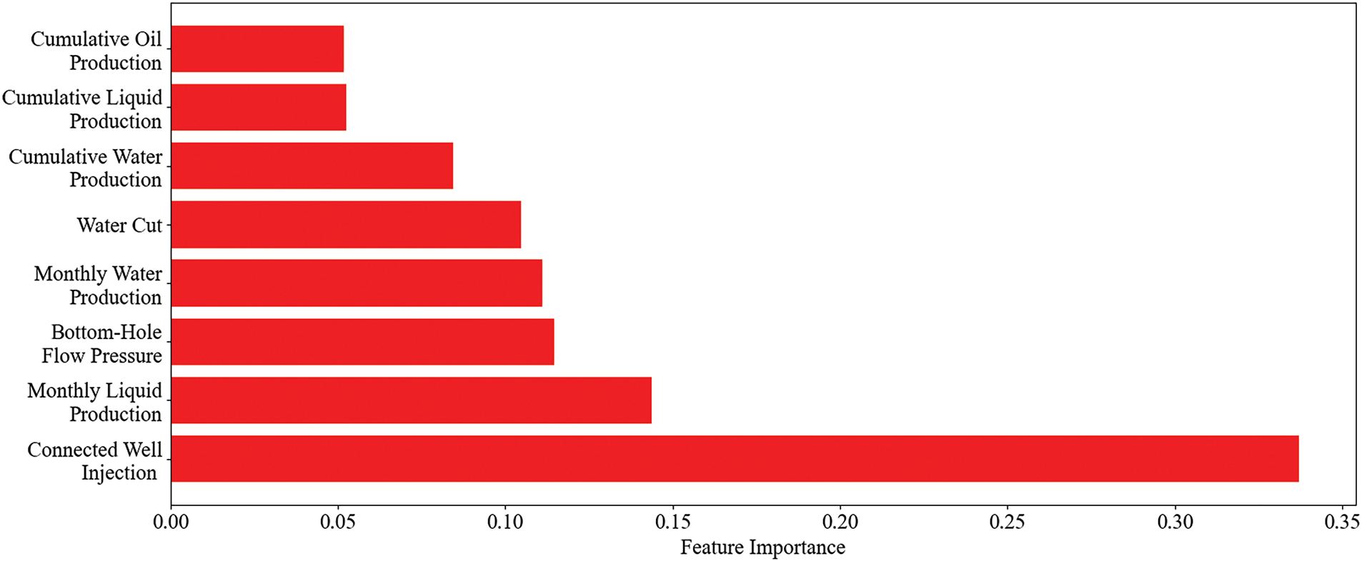
Figure 3: Importance of dynamic production features

5.2 Production Clustering Results

The production data in the training set were clustered using the K-Means clustering algorithm, with the results illustrated in Fig. 4. When the number of clusters is set to 2, the silhouette coefficient achieves a maximum value of 0.793, indicating optimal clustering performance. The category with fewer production wells is designated as Category 1, which includes 6 oil wells, while the category with a greater number is referred to as Category 2, consisting of 44 oil wells.

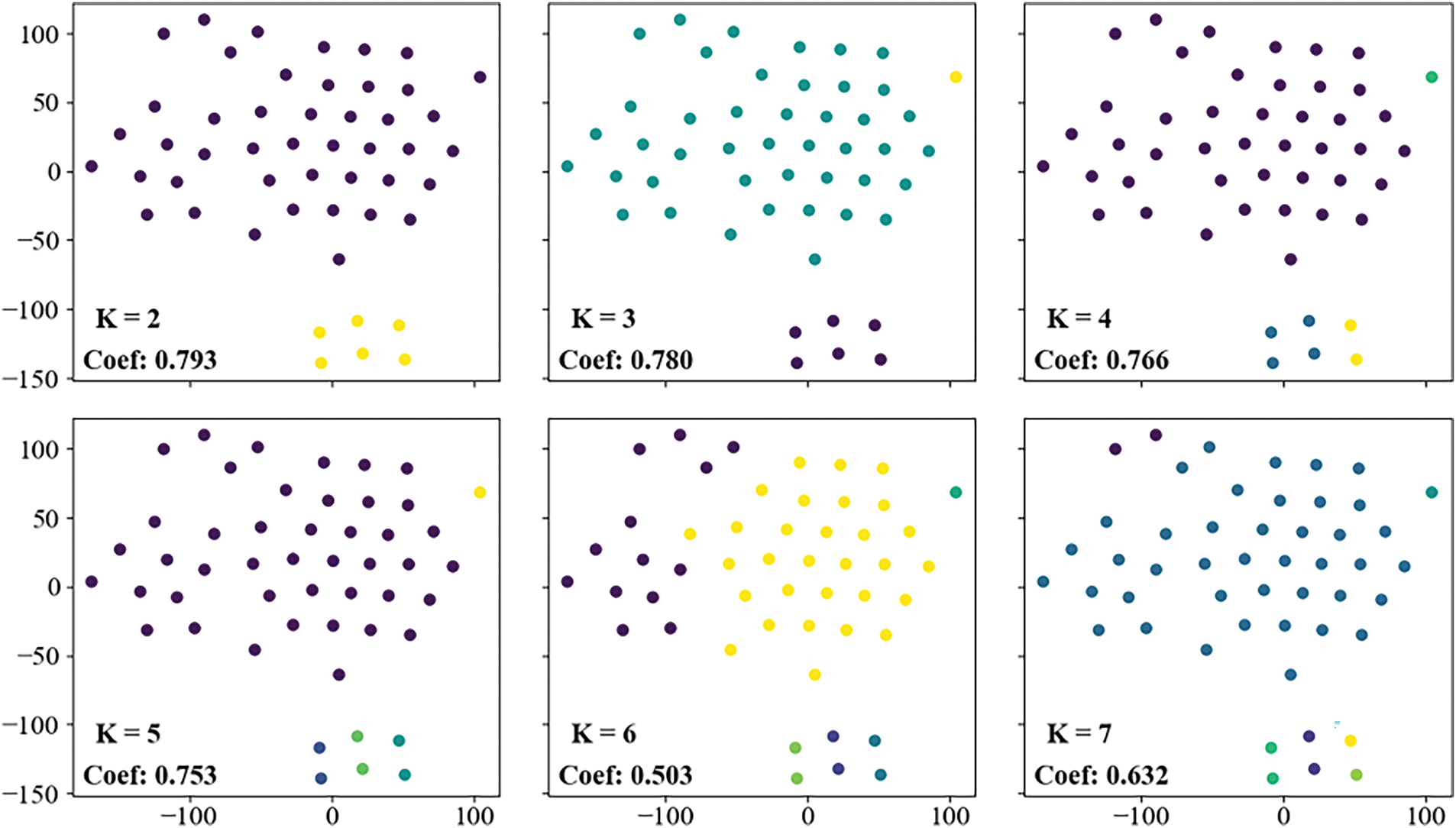
Figure 4: Production clustering results

5.3 Spatial-Geological Matrix Sparsification Results

We constructed the spatial-geological matrix based on the spatial distances and geological feature correlations of production wells, as illustrated in Fig. 5a,b. Afterwards, we applied a base threshold to filter out the lower values in the matrix, thereby focusing our attention on production wells with stronger spatial and geological feature correlations, as shown in Fig. 5c. Finally, to comprehensively account for both inherent and external factors, the SPC algorithm is used to optimize the spatial-geological matrix. By removing certain connections between production wells that belong to different categories based on the inter-class threshold, we achieved a sparse representation of the spatial-geological matrix, as depicted in Fig. 5d.

Figure 5: Spatial-geological matrix sparsification results: (a) Initial spatial-geological matrix; (b) Initial spatial-geological matrix with category distinctions; (c) Spatial-geological matrix with category distinctions, filtered by base threshold; (d) Spatial-geological matrix with category distinctions, with 50% of inter-class connections removed. Note: Blue represents inter-class connections, and red represents intra-class connections

To determine the optimal combination of the base threshold and the inter-class threshold, we employed a grid search method. The SPC effect reached its maximum when the base threshold was set to 0.5, with 50% of the connections between production wells that belong to different categories removed.

5.4 Production Forecasting Results

After the model was established, evaluation metrics were employed to assess its accuracy and generalization capability. In this study, we selected the mean absolute error (MAE), root mean square error (RMSE), and coefficient of determination (R2) as the evaluation metrics:

MAE=1n∑i=1n|yi−y^i|,(13)

RMSE=1n∑i=1n(yi−y^i)2,(14)

R2=1−∑i=1n(yi−y^i)2(yi−y¯)2,(15)

where yi is the actual value of the sample, ŷi is the ith forecasted value, y¯ is the mean value of the sample, n represents the total number of data in the test set.

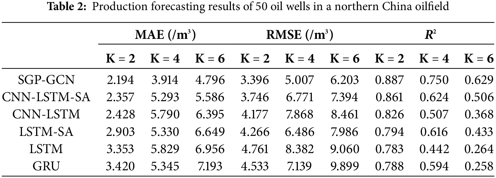
Use SGP-GCN to forecast short-term, medium-term, and long-term production. At the same time, deep learning models such as CNN-LSTM-SA and CNN-LSTM are trained using the same spatio-temporal feature coding. After determining the optimal hyperparameters using the grid search method, a systematic comparison was performed. The experimental results show that SGP-GCN exhibits the highest forecasting accuracy on long-term production forecasting in all study areas, which are shown in Tables 2–4. Meanwhile, we have visualized the long-term forecasting results of SGP-GCN in Appendix A.

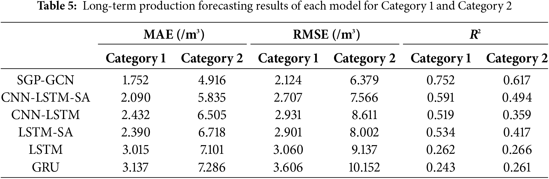
In the message passing process, due to the higher proportion of inter-class connections, production wells in categories with fewer wells are more susceptible to the influence of deviated information. Therefore, in theory, SGP-GCN has more significant advantages in production forecasting of such production wells. We show the long-term production forecasting results for Category 1 and Category 2, as shown in Table 5.

To assess the advantage of SGP-GCN compared to other models in such production wells, we define the relative decrease in mean absolute error (DM), relative decrease in root mean square error (DR) and increase in coefficient of determination (IR) as the evaluation metric:

DM=MAEmodel−MAESGP−GCNMAEmodel,(16)

DR=RMSEmodel−RMSESGP−GCNRMSEmodel,(17)

IR=RSGP−GCN2−Rmodel2,(18)

where MAESGP−GCN, RMSESGP−GCN, and RSGP−GCN2 are mean absolute error, root mean square error and coefficient of determination for SGP-GCN in long-term production forecasting, respectively, MAEmodel, RMSEmodel, and Rmodel2 are mean absolute error, root mean square error, and coefficient of determination for other models in long-term production forecasting.

As shown in Fig. 6, the DM, DR, and IR on Category 1 is higher than the Category 2 in most instances, proving its superiority in dealing with the categories with lesser production wells compared with other models. Specifically, well 4 is a production well in Category 1, and its long-term production forecasting results of each model are shown in Fig. 7. In the long-term production forecasting, all models have some degree of lag. However, the SGP-GCN model is able to sense and respond to dynamic changes in production in a relatively timely manner, thereby providing more accurate production forecasting results.

Figure 6: Comparison of the results of the long-term production forecasting for Category 1 and Category 2: (a) Comparison of DM; (b) Comparison of DR; (c) Comparison of IR

Figure 7: Long-term oil production forecasting results of each model for well 4

5.5 Ablation Experiments

To evaluate the effectiveness of the attention mechanism, spatial distance matrix S, geological feature matrix G, spatial-geological matrix A, and the SPC algorithm in enhancing the accuracy of production forecasting, we conducted ablation experiments on the components mentioned above, with the results shown in Table 6. Here, “w/oSA” represents for SGP-GCN without the attention module. “w/oS”, “w/oG”, and “w/oA” indicate that the matrices S, G, and A are encoded as all-one matrices in SGP-GCN, respectively, while “w/oSPC” indicates that the SPC algorithm is not applied in SGP-GCN.

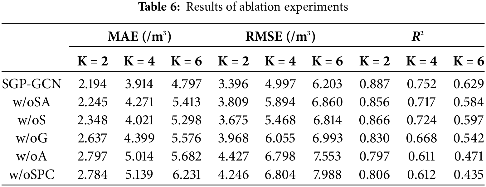
The experiment results show that adding the attention mechanism to SGP-GCN helps to improve the accuracy of petroleum production forecasting at each step. The short-term and medium-term production forecasting results demonstrate that matrices S, G, and A can introduce spatial and geological information during the message passing process, significantly improving forecasting accuracy. In the short-term production forecasting, the RMSE was reduced by 0.279, 0.572, and 1.031, respectively; in the medium-term production forecasting, the RMSE was reduced by 0.471, 1.058, and 1.801, respectively. This emphasizes that even static geological features evolve throughout the development process. Our findings reveal that production wells selected based on geological features before production are more likely to maintain stronger correlations. Prioritizing these wells can lead to improved forecasting performance compared to treating all production wells with equal consideration.

However, as the forecasting step further increases, the deviated information introduced by matrix A gradually becomes a prominent negative factor affecting the accuracy of production forecasting. In this context, the introduction of SPC algorithm can effectively address the production and geological features variations caused by external factors, leading to a significant reduction of 1.785 in the RMSE.

5.6 Computational Cost

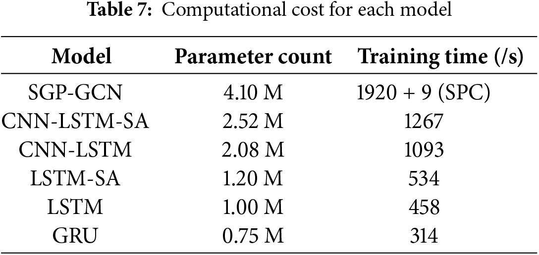
We conducted a comparative analysis of the parameter counts and training times across various models, as shown in Table 7. The experiments were carried out on a machine equipped with 2 Intel Xeon Silver 4316 CPUs, 3 NVIDIA Geforce RTX 3090 GPUs, and 128 GB of memory. Overall, the SGP-GCN had a higher parameter count compared to the other models, which resulted in it requiring more time during the training process. Additionally, the time required to optimize the spatial-geological matrix using the SPC algorithm also contributed to the longer time cost for the SGP-GCN.

5.7 Hyperparameter Sensitivity

To assess the impact of each hyperparameter on long-term forecasting performance, we conduct sensitivity analyses of the hyperparameters in SGP-GCN, as depicted in Fig. 8. For instance, when the base threshold is set too low, production wells with weak spatial and geological feature correlation disproportionately dominate the attention weights in SGP-GCN, which undermines the focus on production wells with stronger spatial and geological feature correlations. Conversely, if the base threshold is set too high, valuable information for long-term production forecasting from production wells exhibiting strong spatial and geological feature correlations may be overlooked.

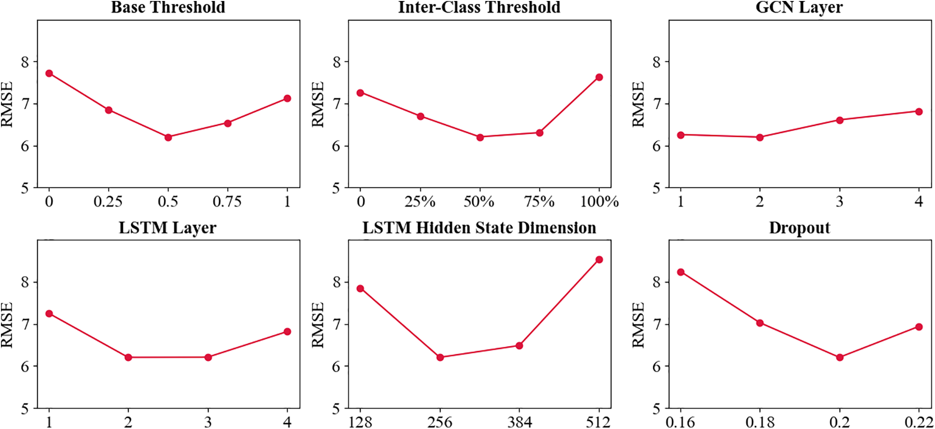
Figure 8: Hyperparameter sensitivity analysis results

6  Conclusions

This study establishes the relationships between production wells based on the synergy of spatial distance and geological feature correlations, developing a spatial-geological perception graph convolutional network (SGP-GCN) for long-term petroleum production forecasting. Additionally, a matrix sparsification algorithm based on production clustering (SPC) is introduced. By reducing attention on production wells with significant production discrepancies, this approach can reduce the influence of deviated information, thereby enhancing the accuracy of long-term production forecasting.

Experimental results demonstrate that, compared to deep learning models such as CNN-LSTM-SA, SGP-GCN exhibits higher accuracy in long-term petroleum production forecasting. Future research will aim to expand the variety of data utilized for encoding the representation of production wells and constructing the adjacency matrix. Specifically, we will explore the integration of artificial control factors, such as well stimulation, into the representation of production wells to improve the adaptability and predictive capability of SGP-GCN.

7  Discussions

•   Scalability: SGP-GCN can be applied to various resource extraction industries where production is closely linked to geological features and other relevant factors. The fundamental approach involves modeling diverse extraction points (e.g., mineshafts and geothermal wells) within the same study area as nodes in a graph. By analyzing the correlations among geological and other relevant features, we can construct a weight matrix that facilitates the selective integration of information from multiple extraction points. Additionally, the SPC algorithm can be utilized to optimize the existing weight matrix based on known production data, thereby updating the weight distribution for information integration. Through this methodology, SGP-GCN has the potential to deliver accurate long-term production forecasts for other resource extraction industries.

•   Deployment challenges: In real-world applications, the diversity of well logging techniques results in a wide variety of well logging data formats. Effectively extracting geological features from this diverse data for production wells complicates the application of SGP-GCN. Additionally, production data from different oilfields may exhibit varying sensitivities to the same geological features. This geological heterogeneity indicates that there may be more optimal parameter combinations than those utilized in current experiments. However, the limited quantity of well logging records presents significant challenges for analyzing geological feature sensitivity. Furthermore, compared to models like LSTM, SGP-GCN has a larger number of parameters. As the dataset size increases, the model requires better configuration and longer training times.

Acknowledgement: None.

Funding Statement: This research was funded by National Natural Science Foundation of China, grant number 62071491.

Author Contributions: The authors confirm contribution to the paper as follows: Study conception and design: Xin Liu, Meng Sun; Data collection: Meng Sun, Bo Lin, Shibo Gu; Analysis and interpretation of results: Meng Sun; Draft manuscript preparation: Meng Sun, Xin Liu. All authors reviewed the results and approved the final version of the manuscript.

Availability of Data and Materials: The production data of 6 gas wells in Montney shale oil and gas production area can be available at https://data.mendeley.com/datasets/vdpkty7wrf/1 (accessed on 01 June 2024) and the Volve dataset can be avaliable at https://data.equinor.com/dataset/Volve (accessed on 06 December 2024). Additional data can be obtained by contacting the corresponding author.

Ethics Approval: Not applicable.

Conflicts of Interest: The authors declare no conflicts of interest to report regarding the present study.

Appendix A

The long-term production forecasting results of SGP-GCN for the 6 gas wells in Montney shale oil and gas production area and 5 oil wells in Volve field are shown in Figs. A1 and A2.

Figure A1: Long-term production forecasting results of SGP-GCN for 6 gas wells in Montney shale oil and gas production area

Figure A2: Long-term production forecasting results of SGP-GCN for 5 oil wells in Volve field

References

1. Du J, Zheng J, Liang Y, Ma Y, Wang B, Liao Q, et al. A deep learning-based approach for predicting oil production: a case study in the United States. Energy. 2024;288(4):129688. doi:10.1016/j.energy.2023.129688. [Google Scholar] [CrossRef]

2. Middleton RS, Gupta R, Hyman JD, Viswanathan HS. The shale gas revolution: barriers, sustainability, and emerging opportunities. Appl Energy. 2017;199:88–95. doi:10.1016/j.apenergy.2017.04.034. [Google Scholar] [CrossRef]

3. Nashawi IS, Malallah A, Al-Bisharah M. Forecasting world crude oil production using multicyclic hubbert model. Energy Fuels. 2010;24(3):1788–800. doi:10.1021/ef901240p. [Google Scholar] [CrossRef]

4. Nguyen-Le V, Shin H, Little E. Development of shale gas prediction models for long-term production and economics based on early production data in Barnett reservoir. Energies. 2020;13(2):424. doi:10.3390/en13020424. [Google Scholar] [CrossRef]

5. Wang J, Shi C, Ji S, Li G, Chen Y. New water drive characteristic curves at ultra-high water cut stage. Petrol Explor Dev. 2017;44(6):1010–5. doi:10.1016/S1876-3804(17)30113-1. [Google Scholar] [CrossRef]

6. Li S, Feng Q, Zhang X, Yu C, Huang Y. A new water flooding characteristic curve at ultra-high water cut stage. J Petrol Explor Prod Technol. 2023;13(1):101–10. doi:10.1007/s13202-022-01538-6. [Google Scholar] [CrossRef]

7. Wang Q, Song X, Li R. A novel hybridization of nonlinear grey model and linear ARIMA residual correction for forecasting U.S. shale oil production. Energy. 2018;165:1320–31. doi:10.1016/j.energy.2018.10.032. [Google Scholar] [CrossRef]

8. Song H, Zhu J, Wei C, Wang J, Du S, Xie C. Data-driven physics-informed interpolation evolution combining historical-predicted knowledge for remaining oil distribution prediction. J Petrol Sci Eng. 2022;217(4):110795. doi:10.1016/j.petrol.2022.110795. [Google Scholar] [CrossRef]

9. Noshi CI, Eissa MR, Abdalla RM. An intelligent data driven approach for production prediction. In: Proceedings of the Offshore Technology Conference; 2019 May 6–9; Houston, TX, USA. [Google Scholar]

10. Ng CSW, Jahanbani Ghahfarokhi A, Nait Amar M. Well production forecast in volve field: application of rigorous machine learning techniques and metaheuristic algorithm. J Petrol Sci Eng. 2022;208:109468. doi:10.1016/j.petrol.2021.109468. [Google Scholar] [CrossRef]

11. Sagheer A, Kotb M. Time series forecasting of petroleum production using deep LSTM recurrent networks. Neurocomputing. 2019;323(3):203–13. doi:10.1016/j.neucom.2018.09.082. [Google Scholar] [CrossRef]

12. Lu C, Jiang H, Yang J, Wang Z, Zhang M, Li J. Shale oil production prediction and fracturing optimization based on machine learning. J Petrol Sci Eng. 2022;217(4):110900. doi:10.1016/j.petrol.2022.110900. [Google Scholar] [CrossRef]

13. Han D, Kwon S. Application of machine learning method of data-driven deep learning model to predict well production rate in the shale gas reservoirs. Energies. 2021;14(12):3629. doi:10.3390/en14123629. [Google Scholar] [CrossRef]

14. Du C, Gong F, Zhou Y, Lu Y, Wang H, Gao J. A mechanistic-based data-driven modeling framework for predicting production of electric submersible pump wells in offshore oilfield. Geoenergy Sci Eng. 2025;246(5):213603. doi:10.1016/j.geoen.2024.213603. [Google Scholar] [CrossRef]

15. Li X, Ma X, Xiao F, Xiao C, Wang F, Zhang S. A physics-constrained long-term production prediction method for multiple fractured wells using deep learning. J Petrol Sci Eng. 2022;217:110844. doi:10.1016/j.petrol.2022.110844. [Google Scholar] [CrossRef]

16. Ibrahim NM, Alharbi AA, Alzahrani TA, Abdulkarim AM, Alessa IA, Hameed AM, et al. Well performance classification and prediction: deep learning and machine learning long term regression experiments on oil, gas, and water production. Sensors. 2022;22(14):5326. doi:10.3390/s22145326. [Google Scholar] [PubMed] [CrossRef]

17. Wang H, Mu L, Shi F, Dou H. Production prediction at ultra-high water cut stage via Recurrent Neural Network. Petrol Explor Dev. 2020;47(5):1084–90. doi:10.1016/S1876-3804(20)60119-7. [Google Scholar] [CrossRef]

18. Cheng YF, Yang Y. Prediction of oil well production based on the time series model of optimized recursive neural network. Pet Sci Technol. 2021;39(9–10):303–12. doi:10.1080/10916466.2021.1877303. [Google Scholar] [CrossRef]

19. Liu W, Gu JW. Oil production prediction based on a machine learning method. Oil Drill Prod Technol. 2020;42(1):70–5 (In Chinese). doi:10.13639/j.odpt.2020.01.012. [Google Scholar] [CrossRef]

20. Liu H, Li Y, Du Q, Jia D, Wang S, Qiao M, et al. Prediction of production during high water-cut period based on multivariate time series model. J China Univ Pet. 2023;47(5):103–14 (In Chinese). doi:10.3969/j.issn.1673-5005.2023.05.010. [Google Scholar] [CrossRef]

21. Karim F, Majumdar S, Darabi H, Chen S. LSTM fully convolutional networks for time series classification. IEEE Access. 2017;6:1662–9. doi:10.1109/ACCESS.2017.2779939. [Google Scholar] [CrossRef]

22. Jiang A, Qin Z, Faulder D, Cladouhos TT, Jafarpour B. Recurrent neural networks for short-term and long-term prediction of geothermal reservoirs. Geothermics. 2022;104(2):102439. doi:10.1016/j.geothermics.2022.102439. [Google Scholar] [CrossRef]

23. Zha W, Liu Y, Wan Y, Luo R, Li D, Yang S, et al. Forecasting monthly gas field production based on the CNN-LSTM model. Energy. 2022;260(2):124889. doi:10.1016/j.energy.2022.124889. [Google Scholar] [CrossRef]

24. Pan S, Yang B, Wang S, Guo Z, Wang L, Liu J, et al. Oil well production prediction based on CNN-LSTM model with self-attention mechanism. Energy. 2023;284(6):128701. doi:10.1016/j.energy.2023.128701. [Google Scholar] [CrossRef]

25. Xie F, Zhang Z, Liang L, Zhou B, Tan Y. EpiGNN: exploring spatial transmission with graph neural network for regional epidemic forecasting. In: Proceedings of the Joint European Conference on Machine Learning and Knowledge Discovery in Databases; 2022 Sep 19–23; Grenoble, France. p. 469–85. [Google Scholar]

26. Mao J, Han Y, Tanaka G, Wang B. Backbone-based dynamic spatio-temporal graph neural network for epidemic forecasting. Knowl Based Syst. 2024;296(3):111952. doi:10.1016/j.knosys.2024.111952. [Google Scholar] [CrossRef]

27. Tekin SF, Kozat SS. Crime prediction with graph neural networks and multivariate normal distributions. Signal Image Video Process. 2023;17(4):1053–9. doi:10.1007/s11760-022-02311-2. [Google Scholar] [CrossRef]

28. Ta X, Liu Z, Hu X, Yu L, Sun L, Du B. Adaptive spatio-temporal graph neural network for traffic forecasting. Knowl Based Syst. 2022;242:108199. doi:10.1016/j.knosys.2022.108199. [Google Scholar] [CrossRef]

29. Wang Y, Zheng J, Du Y, Huang C, Li P. Traffic-GGNN: predicting traffic flow via attentional spatial-temporal gated graph neural networks. IEEE Trans Intell Transp Syst. 2022;23(10):18423–32. doi:10.1109/TITS.2022.3168590. [Google Scholar] [CrossRef]

30. LeCun Y, Bottou L, Bengio Y, Haffner P. Gradient-based learning applied to document recognition. Proc IEEE. 2002;86(11):2278–324. doi:10.1109/5.726791. [Google Scholar] [CrossRef]

31. Zhou W, Li X, Qi Z, Zhao H, Yi J. A shale gas production prediction model based on masked convolutional neural network. Appl Energy. 2024;353:122092. doi:10.1016/j.apenergy.2023.122092. [Google Scholar] [CrossRef]

32. Deng S, Wang S, Rangwala H, Wang L, Ning Y. Cola-GNN: cross-location attention based graph neural networks for long-term ILI prediction. In: Proceedings of the 29th ACM International Conference on Information & Knowledge Management; 2020 Oct 19–23; Galway, Ireland. p. 245–54. [Google Scholar]

33. Vaswani A, Shazeer N, Parmar N, Uszkoreit J, Jones L. Attention is all you need. In: Proceedings of the Advances in Neural Information Processing Systems; 2017 Dec 4–9; Long Beach, CA, USA. p. 5998–6008. [Google Scholar]

34. Kim G, Lee H, Chen Z, Athichanagorn S, Shin H. Effect of reservoir characteristics on the productivity and production forecasting of the Montney shale gas in Canada. J Petrol Sci Eng. 2019;182(1):106276. doi:10.1016/j.petrol.2019.106276. [Google Scholar] [CrossRef]

35. Wood JM. Effect of reservoir characteristics on the productivity and production forecasting of the Montney shale gas in Canada: discussion. J Petrol Sci Eng. 2022;208(1):108176. doi:10.1016/j.petrol.2020.108176. [Google Scholar] [CrossRef]

36. Zhang L, Dou H, Wang T, Wang H, Peng Y, Zhang J, et al. A production prediction method of single well in water flooding oilfield based on integrated temporal convolutional network model. Petrol Explor Dev. 2022;49(5):1150–60. doi:10.1016/S1876-3804(22)60339-2. [Google Scholar] [CrossRef]