Low-Carbon Economic Dispatch Strategy for Integrated Energy Systems under Uncertainty Counting CCS-P2G and Concentrating Solar Power Stations

1  Introduction

An integrated energy system (IES) is characterized by the internal integration of multiple energy sources, primarily gas flow and electric current. This system is further augmented by energy storage and conversion equipment, facilitating the realization of multi-energy complementary coexistence, synergistic optimization, and gradient utilization [1]. Given the intricate nature of IES architecture and the heterogeneity of load profiles, an integrated energy system leveraging distributed renewable energy as its core component can meet the demands of diverse load types, thereby enhancing the low-carbon efficiency of IES and the rate of renewable energy consumption [2,3].

Integrated Energy Systems (IESs) pursue decarbonized operation via two key technical routes: indirect and direct emission reduction [4]. In the area of indirect emission cuts, the combined heat and power (CHP) unit, a central power-generating element in IES, shows a distinct heat-power linkage, causing significant carbon discharges. To address this, ramping up the use of renewable energy along with incorporating energy storage systems is vital. These strategies facilitate a well-planned shift in energy consumption timing, ultimately trimming the IES’s indirect carbon footprint [4,5].

For direct emission reduction, carbon sink measures and market trading policies present feasible solutions. Carbon capture and storage (CCS) systems have been proven to perform large-scale, efficient carbon capture [6]. Power-to-gas (P2G) technologies, which tap into leftover renewable energy, offer a promising means to boost renewable energy utilization and lower emissions [7]. Multiple research efforts have explored the carbon reduction benefits of CCS and P2G. For instance, reference [8] designed an all-around coordinated optimization model for P2G-carbon capture power plants. Since gas-fired units are major carbon emitters, treating their CO₂-laden flue gas properly is indispensable. Reference [9] illustrated how CO₂ captured from gas-fired co-generation plants can be sent to electric-to-gas conversion gear for gas synthesis and then recycled back, cutting carbon emissions, gas purchases, and wasted wind power simultaneously. Reference [10] merged CCS with waste incineration power plant flue gas treatment for load adjustment, relying on the integration of CCS and P2G to ease the impacts of renewable energy fluctuations. Moreover, scholars in reference [11] paired P2G with CCS and extended this pairing to complex, multi-energy-source IES. By contrast, reference works [12,13] separated CO₂ capture and utilization processes by connecting P2G and CCS via carbon storage devices. References [14,15] set up CCS setups with liquid storage equipment, which disentangle carbon absorption and regeneration, providing broader output regulation scope and more peaking flexibility. To tackle the high energy costs of carbon capture, reference [16] put forward a flexible capture operation mode to modulate the capture degree of carbon capture equipment, deferring the associated energy expenses over time. However, within the CCS-P2G coupled system, the electro-hydrogen conversion process, other hydrogen application methods, and methanation inefficiencies are often overlooked, and the combination with the carbon trading low-carbon mechanism has yet to be considered.

As shown in reference [17], an optimal CHP model scheduling method based on CCS-P2G was established, solving carbon source and emission issues for CHP unit output. Reference [18] built an integrated wind-PV-hydrogen power system, facilitating renewable energy use and reliable H2 supply in IES. The CCS-P2G coupling model turned carbon trading costs positive, promoting carbon sinks, cutting IES costs, and increasing trading revenues. The Carbon Emission Trading (CET) mechanism [19,20] supports furthering renewable energy consumption and IES low-carbon potential. Some literature, like reference [21], has explored CET’s benefits in IES operations via a cross-regional optimal dispatch model integrating CET and Green Certificate Trading. Reference [22] built an IES dispatch model using the stepped CET mechanism and multi-energy response, showing 6.7% carbon and 9.21% cost reductions. Yet, existing literature has limitations. It separately considers IES equipment’s carbon reduction potential and the trading market, ignoring combined low-carbon tech-policy benefits. Also, the CCS-P2G model overlooks the power-to-hydrogen stage and other hydrogen utilization paths. To fix this, this paper will propose a two-stage P2G model and use gas doping to enhance hydrogen use, applying the stepped CET mechanism for IES decarbonization research.

Concentrating solar power (CSP) is a new solar power generation mode, that integrates photothermal conversion, thermal storage, and synchronous power generation. In integrated energy system research, many scholars focus on CSP. Reference [22] pioneered in clarifying its basic features, laying the foundation for later work. For power system optimal scheduling, reference [23] built a two-stage stochastic model for power systems with CSP, aiming to cut operating costs, highlighting CSP’s value in high-proportion new energy grids. References [24,25] studied photovoltaic power plants in Gansu, Qinghai, etc., evaluating their power generation and flexibility benefits. In grid scheduling, reference [26] proposed coordinating photovoltaic, wind, and thermal power. Electric heating devices convert unused wind power to heat, store it in the photovoltaic plant’s thermal storage, and reuse it, enhancing the plant’s value. References [27–29] adjusted photovoltaic output and paired it with thermal storage operations to suppress wind-solar-storage power fluctuations and promote joint frequency regulation, bringing economic and capacity benefits. To ensure power system stability, reference [30] developed a wind-solar-photothermal combined power generation system model, making grid-connected power match the dispatch curve, and strengthening operation reliability. Reference [31] exploited the complementary regulation characteristics of thermal and photovoltaic power to build a coordinated dispatch model, reducing abandoned new energy and dispatch costs.

Presently, the main analytical methods for uncertainty optimization are the fuzzy chance constraint, robust optimization, and multi-scenario stochastic optimization [32]. Many studies use these to analyze system source-load uncertainties. In reference [33], fuzzy chance constraints handle wind power and load uncertainties, while optimization hierarchy analysis addresses multi-objective functions in a Regional Integrated Energy System (RIES) with pumped storage, wind, hydro, and thermal power units. The model boosts the RIES’s integrated performance. Another study focuses on a multi-timescale cross-provincial grid scheduling strategy for PV-load uncertainties. A VAR model forecasts PV output [34]; multi-scenario stochastic optimization analyzes day-ahead PV uncertainty; a trapezoidal fuzzy number equivalence model examines intraday uncertainties. This strategy cut’s intraday fuzzy chance constraint complexity raises PV cross-provincial consumption via pumped storage and optimizes PV output and load differences between provinces. In reference [35], the multi-energy virtual power plant model, considering carbon capture and storage, uses fuzzy numbers to study wind and load uncertainties’ impact on carbon capture. The model reduces system carbon emissions. Reference [36] looks at a MEH energy scheduling scheme with carbon emissions in mind, generating multiple scenarios via the probability density function to assess renewable energy output uncertainties. Reference [37] explores a day-ahead optimal scheduling model with multi-scenario analysis, using improved K-means clustering for scenario generation and reduction to shorten computation time. Reference [38] studies an MMG two-tier scheduling strategy for wind-scenic cooperative energy storage, establishing power balance constraints with uncertain parameters and introducing slack power constraints to cut power supply-demand deviation. Finally, reference [39] examines a coupled electricity-carbon MMG cooperative game optimization scheduling model with multiple uncertainties, applying the opportunity constraint method to wind power output uncertainty and robust optimization to tariff uncertainty.

In summary, although research on low-carbon operation of IES has made some progress, existing studies have neglected the stability problem of renewable energy generation. In IES containing a high proportion of renewable energy, the disturbance problems caused by the fluctuation and randomness of renewable energy generation cannot be ignored. To promote the low-carbon operation of IES and improve the disturbance-resistant capability of IES, this paper proposes a low-carbon economic dispatch study of IES under uncertainty taking into account CCS-P2G and CSP station, with the following steps: (1) a low-carbon dispatch model of IES based on CCS-P2G, CSP station and gas hydrogen doping unit is established, and the effectiveness of the gas hydrogen doping and variable hydrogen doping ratio modes are analyzed; (2) the ladder-type carbon trading mechanism into IES, and conducted sensitivity analysis of the carbon trading benchmark price of IES and its growth rate; (3) used trapezoidal fuzzy numbers to relax the IES power balance constraints and transform them into clear equivalence classes, and established the IES optimal scheduling strategy based on the fuzzy opportunity constraints; (4) used weight coefficients as the risk assessment indexes, and established the IES risk assessment based on the CVaR strategy. Finally, the simulation example shows that the proposed strategy effectively reduces the operation cost and carbon emission of IES, the carbon trading base price of IES and its growth rate jointly decide the carbon emission of IES, and the anti-disturbance ability of IES is evaluated by the trapezoidal fuzzy number and CVaR.

2  IES Model with CCS-P2G, Gas-Fired Hydrogen-Doped Units and CSP

The IES in this paper consist of a thermal unit (TU), gas turbine (GT), gas boiler (GB), P2G, CSP power plant, wind turbine (WT), CCS and electric energy storage, and the load consists of electric and thermal loads. The structure of IES in this paper is shown in Fig. 1:

Figure 1: IES structure diagram

2.1 Mechanisms and Models for Coupled CCS-P2G Operation

2.1.1 Mechanisms and Models of CCS Operation

The introduction of a flue gas diverter system and liquid storage vessel in CCS forms an integrated and flexible operation mode of CCS [40], which improves the flexibility of its operation in conjunction with P2G. Gas boilers, gas turbines, and thermal power units all generate CO2 during operation, and in the CCS-P2G coupled operation mode proposed in this paper, the CCS collects the captured CO2 and transports it to the methane reactor (MR) for methanation, which reduces the cost and carbon emission of purchasing CO2 from external sources by the IES and avoids the leakage of CO2 during the transportation to the CCS or CCUS. It also avoids the leakage of CO2 during transportation to CCS or CCUS, which may cause environmental pollution [41]. Fig. 2 shows the energy flow diagram of the coupled CCS-P2G operation mode:

Figure 2: Energy flow diagram of CCS-P2G coupled gas hydrogen doping system

The actual capture energy consumption of CCS in the time t PtCCS consists of the operational energy consumption Pt,bCCS and the stationary energy consumption Pt,dCCS [42]:

{PtCCS=Pt,bCCS+Pt,dCCSPt,bCCS=ωCCSPt,CO2CCS,m(1)

where ωCCS is the energy consumption per unit mass of CO2 captured by CCS, taken as 0.269 MW⋅h/t; Pt,CO2CCS,m is the mass of CO2 captured by the CCS regeneration tower during the time t.

The CCS contains a flue gas splitter system that increases CCS operational flexibility and reduces energy consumption by actively venting CO2 into the atmosphere as required by the IES:

Pt,CO2IES=Pt,CO2CCS+Pt,1air(2)

where Pt,CO2IES is the total amount of CO2 emitted by the IES during the time t; Pt,CO2CCS is the amount of CO2 absorbed by the CCS during the time t; Pt,1air is the amount of CO2 discharged from the CCS to the atmosphere via the flue gas splitter system during the time t.

The decoupling of the CO2 absorption and regeneration processes is realized by installing a liquid storage vessel between the absorption and regeneration towers and transferring the CCS energy consumption by adjusting the liquid storage volume of the vessel. The CCS energy consumption is reduced when the liquid-rich unit has more liquid storage and the liquid-poor unit has less liquid storage and vice versa, which is modelled as follows:

{VtF=Vt−1F+Vt,inF−Vt,outFVtP=Vt−1P+Vt,inP−Vt,outPVt,inF=Vt,outPVt,outF=Vt,inP(3)

where VtF and VtP are the volume of liquid storage in the liquid-rich vessel and the liquid-poor vessel in the time t, respectively; Vt,inF and Vt,outF are the volume of inflow and outflow from the liquid-rich vessel in the time t, respectively; Vt,inP and Vt,outP are the volume of inflow and outflow from the liquid-poor vessel in the time t, respectively.

In this paper, we use the form of the volumetric amount of solution instead of a CO2 amount, if a unit volume of enriched liquid absorbs 20 times the volume of CO2:

{20Vt,inF=ηCCSPt,CO2CCS/ρCO220Vt,outP=ηCCS(Pt,MRCCS+Pt,storageCCS)/ρCO2(4)

where ηCCS is the CCS capture efficiency, taken as 95%; ρCO2 is the CO2 gaseous density, assuming a temperature of 20°C, ρCO2=770 kg/m3.

The regenerated CO2 is transported to the MR or sequestered, and some is discharged to the atmosphere:

Pt,outCCS=Pt,storageCCS+Pt,MRCCS+Pt,airCCS(5)

where Pt,outCCS is the amount of CO2 produced by CCS in the time t; Pt,MRCCS is the amount of CO2 sequestered at in the time t; Pt,airCCS is the amount of CO2 emitted to the atmosphere after regeneration of CCS in the time t.

2.1.2 Mechanisms and Models for the Two-phase Operation of the P2G

The P2G operation process is divided into two stages: P2H and hydrogen to gas (H2G). In the first stage, the electrolytic (EL) electrolyzes water, realizing the conversion of “electricity-hydrogen energy”; in the second stage, the EL delivers the hydrogen energy to MR, GT, and GB, respectively. Fig. 3 shows the process diagram of the two stages of P2G:

Figure 3: Two-stage operational process of P2G

The MR is mechanized to produce CH4, which can be supplied directly to the gas load or delivered to the CHP or GB to produce electricity/thermal energy. The raw materials consumed by the GT and GB consist of the hydrogen generated by the P2G and natural gas, as well as the gas purchased from an external gas grid. This P2G two-stage model also reduces carbon emissions and improves the efficiency of P2G operation by operating GT and GB with gas-doped hydrogen compared to the conventional P2G model.

The P2G model is as follows:

Pt,H2EL=ηELPtP2G(6)

where PtP2G is the P2G power consumption in the time t; Pt,H2EL is the EL hydrogen production power in the time t; ηEL is the P2H conversion efficiency.

Pt,CH4MR=ηMRPt,H2MR(7)

where Pt,H2MR and Pt,CH4MR are the hydrogen consumption power and gas production power of MR at the time t; ηMR is the MR conversion efficiency.

P2G generates CH4 by a volume equal to the volume of CO2 consumed:

Vt,CH4MR=Pt,MRCCS/ρCO2(8)

P2G generates CH4 volume Vt,CH4MR vs. power consumption PtP2G at the t time slot:

Vt,CH4MR=ηMRPt,H2MRLH2/ρCH4LCH4(9)

where LH2 and LCH4 are the calorific values of H2 and CH4, respectively.

2.2 Operational Modelling of Hydrogen Doping in Gas Turbines and Gas Boilers

2.2.1 Hydrogen-Doped Gas Turbine Model

The standard hydrogen-doped gas turbine can maintain safe operation in the range of 0%~30% hydrogen-doping ratio, beyond which the standard hydrogen-doped gas turbine needs to be improved, which increases the investment cost [43]. Therefore, in this paper, the gas turbine with a hydrogen doping ratio of 10%~20% is selected and modelled as follows:

{Pt,eGT=ηeGTPt,mixGTPt,hGT=ηhGTPt,mixGTPt,mixGT=εCH4vVt,CH4GT+εH2mPt,H2GTλt,H2GT=(Pt,H2GT/ρH2)/[Vt,CH4GT+(Pt,H2GT/ρH2)](10)

where Pt,mixGT is the GT mixed gas input power at time t; Pt,eGT and Pt,hGT are the GT power and thermal generation power at time t; ηeGT and ηhGT are the GT power and thermal generation efficiencies; εCH4v is the volumetric power conversion factor of CH4; εH2m is the mass power conversion factor of H2; Vt,CH4GT and Pt,H2GT are the GT gas and hydrogen consumption at time t; ρH2 is the density of H2.

2.2.2 Modeling of Hydrogen-Doped Gas Boilers

GB can also be doped with a certain amount of H2 operation is modeled as follows:

{PtGB=ηGBPt,mixGBPt,mixGB=εCH4vVt,CH4GB+εH2mPt,H2GBλt,H2GB=(Pt,H2GB/ρH2)/[(Pt,H2GB/ρH2)+Vt,CH4GB](11)

where Pt,mixGB is the gas input power of GB at time t; PtGB is the heating power of GB at the time t; ηGB is the heating efficiency of GB; Vt,CH4GB and Pt,H2GB are the gas consumption and hydrogen consumption of GB at the time t, respectively; λt,H2GB is the hydrogen doping ratio of GB at the time t.

2.3 CSP Plant Model

The CSP station is divided into a concentrating solar collector link, thermal energy storage link and power generation link. The solar field (SF) of the CSP station absorbs solar energy into the collector, and produces high-pressure steam through the heat exchanger to the turbine generator (TG) for power generation, and the remaining thermal energy is stored in the TES, which can be transferred to the TG for power generation or directly supplied to the thermal load when the light intensity is weak or no light is available. The remaining thermal energy is stored in the TES, which can be transferred to the TG for power generation or directly supplied to the thermal load when the solar irradiance is weak. The CSP station will produce light and thermal energy loss during operation, and the degree of loss is related to the material of the TES and the external environment, etc. The CSP station can also be used as a solar energy storage system.

2.3.1 Concentration of Solar and Thermal Collection Links

PtSF=ηSFSSFDt(12)

where PtSF is the absorbed thermal power of the SF at the time t; ηSF is the photothermal conversion rate of the SF; SSF is the area of the SF; Dt is the direct normal irradiance (DNI) of the solar energy at time t, w/m2.

2.3.2 Thermal Storage

The thermal power Et,SFTES supplied to the TES by the SF at time t is:

Pt,SFTES=(1−μnonSF)(PtSF−Pt,SFTG)(13)

where μnonSF is the thermal loss rate of the SF; Pt,SFTG is the power supplied by the SF to the generator at time t.

The following constraints need to be met for the thermal storage segment of a CSP station:

{P1TES=PTTESPtTES=(1−ηnonTES)Pt−1TES+ηcTESPt,cTES−Pt,dTES/ηdTESPt,cTESPt,dTES=0(14)

where P1TES and PTTES are the thermal storage capacity at the beginning and end of a TES scheduling cycle; PtTES is the thermal storage capacity of TES at time t; ηnonTES is the self-loss rate of TES; ηcTES and ηdTES are the TES charging and discharging efficiencies; Pt,cTES and Pt,dTES are the TES charging and discharging power at time t.

TES stored thermal can be used for direct heat loads or for TG generation:

Pt,dTES=Pt,TESTG+Pt,TESL(15)

where Pt,TESTG and Pt,TESL are the thermal power output from TES to TG and thermal loads respectively at time t.

2.3.3 Power Generation

The output electric power PtCSP of the CSP plant at time t is:

PtCSP=ηrdCSP(Pt,SFTG+Pt,TESTG)(16)

where Pt,SFTG is the thermal power output from SF to the TG; ηrdCSP is the thermoelectric conversion rate of the CSP station.

2.4 Electrically Heated Models

Pt,hEH=nEHPt,eEH(17)

where Pt,eEH and Pt,hEH are the electrical power input and thermal power output of the electric heating at time t, respectively; nEH is the electrical-to-thermal conversion rate.

2.5 Energy Storage Modeling

The CSP station thermal storage system model is shown in Eqs. (13)–(15), and the electrical storage station (ESS) model is as follows:

{PtESS=(1−ηnonESS)Pt−1ESS+ηcESSPt,cESS−Pt,fESS/ηfESS0≤ut,cESSPt,cESS≤Pmax,cESS0≤ut,fESSPt,fESS≤Pmax,fESSut,cESSut,fESS=0Pt,minESS≤EtESS≤Pt,maxESS(18)

where PtESS is the ESS storage capacity at time t; ηcESS and ηfESS are the ESS charging and discharging efficiencies; ηnonESS is the ESS self-damage rate; Pt,cESS and Pt,fESS are the ESS charging and discharging powers at time t; ut,cESS and ut,fESS are the ESS charging and discharging status bits, which are 0–1 variables, with 1 being the action, and vice versa, with 0; Pt,minESS and Pt,maxESS are the ESS storage capacity lower and upper limits.

3  Stepped Carbon Trading Mechanism

The carbon trading mechanism renders carbon emissions tradable in the market, enabling parties to trade for emission control. Carbon emission quotas are assigned to IES emitters. If actual emissions exceed the allocated amount, extra quotas must be bought from the market; surplus ones can be sold for income. The stepped carbon trading mechanism consists mainly of the quota, actual emission, and stepped trading models.

3.1 IES Emission Right Quota Model

This paper adopts the baseline method as the indicator of the gratuitous quota model for allocation, this paper IES carbon emission sources are GB, GT and external power purchase, and it is considered that the external power purchase comes from thermal power unit generation. In this paper, IES carbon credits are modeled as:

{EIES=EGT+EGB+EthEGT=γh∑t=1T(χe−hPt,eGT+Pt,hGT)EGB=γhPtGBEth=γthPtth(19)

where EIES, EGT, EGB and Eth are the carbon credits allocated to IES, GT, GB, and TU, respectively; γe is the intensity of carbon credits per unit of electricity output of GT; χe−h is the electricity-thermal conversion factor of GT; γh is the intensity of carbon credits per unit of thermal power output; γth is the intensity of carbon credits per unit of electricity output of thermal power units.

3.2 IES Actual Carbon Emission Model

In this paper, the actual carbon emissions from the IES are the amount of generated CO2 minus the amount of CO2 utilized by P2G and the amount of CO2 sequestered. The amount of CO2 Ptair discharged into the atmosphere by IES at time t is divided into the amount of CO2 discharged into the atmosphere through the flue gas splitter system, Pt,1air and the amount of CO2 that is not utilized by the CCS, Pt,2air.

{Ptair=Pt,1air+Pt,2airPt,2air=(1−ηG)Etc(20)

The actual amount of CO2 generated by the IES Et,IESc is:

Et,IESc=δc(Et,CH4GB+Et,CH4GT)+δthPtth(21)

where δc is the carbon intensity per unit of CH4 consumed; δth is the carbon intensity per unit of the power output of thermal power units; Et,CH4GB and Et,CH4GT are the power consumption per unit of CH4 consumed by GB and GT respectively at time t.

3.3 IES Ladder-Type Carbon Trading Mechanism Model

By solving for the IES carbon allocation Et,IES and the IES actual carbon emission Et,IESc in time period t, the IES carbon trading amount Et,IESjt can be obtained:

Et,IESjt=Et,IESc−Et,IES(22)

To impose further limitations on IES carbon emissions, this paper employs a stepped carbon trading model. In contrast to the conventional carbon trading pricing model, this model employs distinct carbon trading prices across various carbon emission intervals. The magnitude of the carbon trading price within a specific interval is directly proportional to the quantity of carbon emission rights allocated. The specific structure of the stepped carbon trading model is outlined as follows:

ft,CO2={λEt,IESjt,Et,IESjt≤lλ(1+α)(Et,IESjt−l)+λl,l<Et,IESjt≤2lλ(1+2α)(Et,IESjt−2l)+(2+α)λl,2l<Et,IESjt≤3lλ(1+3α)(Et,IESjt−3l)+(3+3α)λl,3l<Et,IESjt≤4lλ(1+4α)(Et,IESjt−4l)+(4+6α)λl,4l<Et,IESjt(23)

where ft,CO2 is the cost of carbon trading at time t; λ is the base price of carbon trading; l is the length of the carbon emission interval; α is the increase in the price of carbon trading.

4  IES Optimized Scheduling Model

4.1 IES Low Carbon Economics Scheduling Model

The goal of the IES low carbon economics scheduling in this paper is to minimize the IES operating costs F1:

minF1=fCO2+ff+fg+fth1+fth2+fyw(24)

where fCO2, ff, fg, fth1, fth2 and fyw are the carbon trading cost, carbon sequestration cost, gas purchase cost, thermal power unit start-up, shut-down cost, thermal power unit coal consumption cost, and operation and maintenance cost of each unit of IES, respectively.

fCO2=∑t=1Tft,CO2(25)

ff=cf∑t=1TPt,storageCCS(26)

fg=cg∑t=1TPt,bg(27)

fth1=sth∑t=2T[utth(1−ut−1th)+ut−1th(1−utth)](28)

fth2=∑t=2T[ath(Ptth)2+bthPtth+cth](29)

fyw=∑t=1T(cywWTPtWT+St,ywCSP+cywEHPt,eEH+cywP2GPtP2G+cywCCSPtCCS+StGT+cywGBPtGB+cywESSPtESS)(30)

St,ywCSP=cyw,eCSPPtCSP+cyw,hCSP(Pt,cTES+Pt,dTES)(31)

StGT=utGT(syw,eGTPt,eGT+syw,hGTPt,hGT)(32)

where cf is the sequestration cost per unit mass of CO2; cg is the unit price of natural gas; Pt,bg is the purchased power of IES at time t; sth is the thermal unit start/stop cost coefficient; utth is the thermal unit start/stop status bit, a 0–1 variable; ath, bth, and cth are the cost factors of coal consumption of thermal units; cywWT, cywEH, cywP2G, cywCCS, cywGB, and cywESS are the operation and maintenance (O&M) costs factors at time t of WT, EH, P2G, CCS, GB, and ESS, respectively; St,ywCSP, StGTare the O&M cost factors of the CSP plant and GT at time t, respectively; cyw,eCSP and cyw,hCSP are the O&M cost coefficients for CSP power generation and storage-exchange thermal, respectively; syw,eGT and syw,hGT are the O&M cost coefficients for GT power generation and thermal generation, respectively; utGT is the GT start-stop status bit, which is a 0–1 variable.

4.2 IES Optimal Scheduling Model Based on Fuzzy Chance Constraints

The notion of opportunity constraints has the capacity to articulate the confidence level of the system. Moreover, the decision scheme can incorporate risk and cost in an uncertain environment. However, it is imperative to acknowledge that the reasonable measurement function exerts a direct influence on the expression of the confidence level. Consequently, the selection of this function must be endowed with a clear physical meaning and practical value. Conventional chance-constrained planning is exclusively for stochastic environments; however, the absence of the row-medium law signifies that wind power also possesses considerable ambiguity [44–46].

Decision-making processes based on fuzzy sets permit adjustments within a specific fuzzy range. Confronted with the inherent uncertainty associated with wind power, decisions pertaining to grid scheduling and energy storage allocation can be made without being constrained by predetermined thresholds. In circumstances where extreme weather events, characterized by their rarity but severe consequences, are difficult to predict with accuracy, the employment of fuzzy decision rules facilitates a swift response, thereby mitigating the potential for complete cessation of energy supply. This approach deviates from conventional deterministic or random strategies by employing a more adaptable and agile decision-making process.

Compared with complex probabilistic statistical analysis, fuzzy set operations rely on the affiliation function and the rules are relatively simple. In the context of large-scale wind power integration into the power system, the fuzzy set method has been shown to have a low computational demand and to facilitate rapid decision-making, thereby assisting dispatchers and maintenance personnel in responding in a timely manner and enhancing system control efficiency. In this section, we propose a methodology that utilizes fuzzy opportunity constraints to relax IES power balance constraints, and trapezoidal fuzzy numbers to convert these constraints into clear equivalence classes. The utilization of fuzzy chance constraints stipulates that the feasibility of the decision outcome satisfying the constraints is not less than the specified confidence level. In the absence of light, the thermal storage system of the CSP plant can maintain stable power generation for an extended period, thereby mitigating the impact of weather uncertainty [47]. This section focuses exclusively on wind power output and load, both of which are subject to uncertainty.

4.2.1 Trapezoidal Fuzzy Numbers

This chapter uses trapezoidal fuzzy numbers for fuzzy planning, which is modeled as follows [34]:

S(ϖ)={ϖ−r1r2−r1,r1≤ϖ≤r21,r2≤r3ϖ−r3r3−r4,r3≤ϖ≤r40,other(33)

where S(ϖ) is the fuzzy affiliation function; ϖ is the fuzzy parameter; r1, r2, r3 and r4 are the fuzzy affiliation parameters, r1≤r2≤r3≤r4.

Trapezoidal fuzzy number characterization using quaternions:

I=(r1,r2,r3,r4)=Ppre(j1,j2,j3,j4)

where I is the trapezoidal fuzzy array; Ppre is the predicted value; j1, j2, j3 and j4 are the scaling coefficients; all belong to [0, 1].

4.2.2 Clear Equivalence Class Modeling

Since the trapezoidal fuzzy array characterized by the quaternion cannot be solved linearly, the transformation method of the reference [34] is used to separate the fuzzy variables from the decision variables and to prove that there is a linear relationship between the two, as described in the reference [34].

Set the confidence level to α, and the clear equivalence class is modeled as:

E[P]=1−α2(r1+r2)+α2(r3+r4)(34)

Therefore, the clear equivalence model for wind power and load in this paper is:

{E[Pt,preWT]=1−α2(r1WT+r2WT)+α2(r3WT+r4WT)E[PtL]=1−α2(r1L+r2L)+α2(r3L+r4L)(35)

riWT=jiPt,preWT,i∈[1,4](36)

riL=jiPtL,i∈[1,4](37)

where r1WT, r2WT, r3WT and r4WT are wind power output trapezoidal fuzzy numbers; r1L, r2L, r3L and r4L are load trapezoidal fuzzy numbers. Eq. (35) is brought into Eqs. (41) and (42) and relaxed to determine the equivalence constraints.

4.3 IES Risk Assessment Model Based on Conditional Value-at-Risk Theory

In this paper, the IES presents a high proportion of renewable energy characteristics. However, due to the volatility and stochasticity of renewable energy output, there is a risk in optimizing dispatch based on forecast data. To enhance the IES’s capacity to manage uncertainties, a risk assessment model is developed in this section. This model is based on conditional value-at-risk (CVaR) theory.

VaR cost fVaR and CVaR cost fCVaR for:

{fVaR(x)=min{y∈R:δ(x,y)≥α}fCVaR(x)=[∫f(x,y)≥fVaR(x)f(x,y)P(y)dy]/1−α(38)

where x and y are the decision variables and random variables, respectively; α is the confidence level, which characterizes the IES decision maker’s liking or disliking of risk; P(y) is the continuous probability density function; and δ(x,y) is the distribution function of f(x,y) which is smaller than the boundary value.

Discretization of Eq. (35):

minF2=fVaR+∑n=1Nznmax[0,f(x,yn)−fVaR]1−α(39)

where fVaR is the VaR cost; α is the confidence level; n is the number of cases; zn is the probability of case n occurrence.

Modeling CVaR-based IES risk assessment:

{minF2=φfE+(1−φ)fCVaR(x,fVaR)fE=∑t=1T∑nNznF1n(40)

where F2 is the total IES operating cost based on CVaR; φ is the weighting factor; fE is the IES expected operating cost; and F1n is the total IES operating cost under case n.

In this article, the weight coefficients are set using a subjective method. In practical applications, the weight coefficients represent the degree of aversion to risks in the project. Since the judgment criteria for risks vary in actual systems and are difficult to quantify through objective methods, the setting method we adopt can also intuitively reflect the effectiveness of this risk assessment system. In this paper, we ignore the effect of solar variations on the output of CSP plants [29], only the effect of uncertainty factors on WT output is considered.

4.4 Constraints

4.4.1 Power Balance Constraints

The IES is internally coupled with electrical, thermal, gas, and hydrogen energy and is constrained to maintain a balance of load and equipment supply:

Pt,eGT+PtWT+PtCSP+Pt,cESS+Ptth=PtP2G+Pt,eEH+Pt,eL+Pt,dESS+PtCCS(41)

Pt,hGT+PtGB+Pt,cTES+Pt,hEH=Pt,dTES+Pt,hL(42)

Pt,CH4GT+Pt,CH4GB=Pt,outCCS+Pt,bg(43)

Pt,H2GT+Pt,H2GB+Pt,H2MR=Pt,H2EL(44)

where PtWT is the WT output power at time t; Pt,eL and Pt,hL are the IES electrical and thermal loads at time t, respectively.

4.4.2 IES Device Constraints

1)   WT and CSP plant output constraints:

{0≤PtWT≤Pt,preWT0≤PtCSP≤Pt,preCSP(45)

where Pt,preWT and Pt,preCSP are the predicted values of WT and CSP at time t, respectively.

2)   Gas turbine and gas boiler output and climb constraints:

{Pt,e,minGT≤Pt,eGT≤Pt,e,maxGTPt,h,minGT≤Pt,hGT≤Pt,h,maxGTΔPe,minGT≤Pt,eGT−Pt−1,eGT≤ΔPe,maxGTΔPh,minGT≤Pt,hGT−Pt−1,hGT≤ΔPh,maxGT(46)

where Pt,e,maxGT and Pt,e,minGT are the upper and lower limits of GT output electric power; Pt,h,maxGT and Pt,h,minGT are the upper and lower limits of GT output thermal power at time t; ΔPe,minGT and ΔPe,maxGT are the upper and lower limits of GT output electric power creep; ΔPh,minGT and ΔPh,maxGT are the upper and lower limits of GT output thermal power creep, respectively.

{PminGB≤PtGB≤PmaxGBΔPminGB≤PtGB−Pt−1GB≤ΔPmaxGB(47)

where PmaxGB and PminGB are the upper and lower limits of GB output thermal power for the t time slot; ΔPmaxGB and ΔPminGB are the upper and lower limits of GB output thermal power creep, respectively.

3)   Electrically heated restraints:

{Ph,minEH≤Pt,hEH≤Ph,maxEHΔPh,minEH≤PtEH−Pt−1EH≤ΔPh,maxEH(48)

where Ph,maxEH and Ph,minEH are the upper and lower limits of EH output thermal power; ΔPh,maxEH and ΔPh,minEH are the upper and lower limits of EH output thermal power creep, respectively.

4)   Thermal unit constraints:

{utthPminth≤Ptth≤utthPminthΔPminth≤Ptth−Pt−1th≤ΔPmaxth(49)

where Pmaxth and Pminth are the upper and lower limits of the output power of thermal power units; ΔPmaxth and ΔPminth are the upper and lower limits of the output power of thermal power units, respectively.

5)   Carbon capture constraints:

CCS operation cannot exceed the maximum operating power Pt,maxCCS:

0≤PtCCS≤Pt,maxCCS(50)

The CCS reservoir vessel is required to meet the following constraints:

{VminF≤VtF≤VmaxFVminP≤VtP≤VmaxP(51)

where VmaxF and VminF are the upper and lower limits of the storage capacity of the liquid-rich container; VmaxP and VminP are the upper and lower limits of the storage capacity of the liquid-poor container; V0F and VTF are the beginning and end storage capacity of the liquid-rich container; V0P and VTP are the beginning and end storage capacity of the liquid-poor container, respectively.

The CCS storage vessel has the same storage capacity at the beginning and end of a dispatch cycle:

{∑t=1T(Vt,inF−Vt,outP)=0∑t=1T(Vt,inP−Vt,outP)=0(52)

6)   P2G constraints:

{PminP2G≤PtP2G≤PmaxP2GΔPminP2G≤PtP2G≤ΔPmaxP2G(53)

7)   Remaining constraints:

The CSP plant thermal storage system cannot operate at full capacity 24 h:

0≤PtTES≤tmaxPtCSP/ηrdCSP(54)

where tmax is the maximum number of hours of full-load operation of the thermal storage system of the CSP plant.

4.5 Model Solving

The IES low-carbon optimal dispatch model in this paper, considering CCS-P2G and concentrating solar power plants under the stepped carbon trading system, is a mixed-integer nonlinear one. We use the segmental linearization method to turn it into a mixed-integer linear model, then solve it with the CPLEX commercial solver. The specific linearization process is detailed in Appendix A.

5  Example Analysis

5.1 Parameters of the Algorithm

The internal structure of IES in this paper is shown in Fig. 1, containing 1 WT, 1 CSP station, 1 GB, 1 GT, 1 P2G, 1 CCS, 1 EH, 1 TU, and 1 ESS. The carbon trading in the IES has a base price of 200 yuan per ton, an interval of 50 tons, and a growth rate of 25%. The price of natural gas is set at 3.2 yuan per cubic meter, while the price of coal for the thermal power unit is 500 yuan per ton. the mass of CH in 1 m is 0.715 kg; the mass of CO in 1 m is 1.95 kg; the mass of H unit coal price is 500 yuan/t; 1 m3 of CH4 mass of 0.715 kg; 1 m3 of CO2 mass of 1.95 kg; 1 m3 of H2 mass of 0.09 kg; 1 kw⋅h consumes 0.3 kg of coal and produces 0.795 kg of CO2. It is postulated herein that the IES operates independently, without interaction with the external power grid. The equipment parameters of the IES are presented in Table A1, the operational parameters of the CSP plant are in Table A2, and the remaining parameters can be found in Table A3. Fig. A1 showcases the predicted values of electric and thermal loads, wind power, and direct normal irradiance (DNI).

5.2 IES Power Balance Analysis

As Fig. 4 shows, IES power goes mainly to electric loads, heating, ESS charging, CCS, and P2H. At night, when the wind is strong, the WT and gas turbine power the IES, and the ESS stores spare wind power. After 6:00, as solar intensity rises, the CSP plant starts generating, peaking from 11:00 to 13:00. This peak load time makes thermal units emit more carbon. So, the CCS captures carbon, and the ESS discharges to add power. Between 18:00 and 21:00, the IES mainly powers the CSP’s thermal storage, cutting thermal unit output. During dispatch, the CSP plant provides stable power at peaks and low-solar times, keeping the IES stable. High thermal output triggers CCS to capture carbon for the IES cycle. The ESS quickly stores/discharges to shift electric power. IES thermal energy goes to loads and the CSP’s thermal storage. At night’s peak, the storage releases heat; in the morning, it stores heat, using its fast heat shift to exploit the CSP’s flexibility. The CO2 balance is in Fig. A2a, and the CCS power balance in Fig. A2b.

Figure 4: IES power balance

5.3 Analysis of Gas Hydrogen Doping Models

5.3.1 Analysis of the Effectiveness of the Gas Hydrogen Doping Model

To verify the effectiveness of the gas-hydrogen doping mode proposed in this paper, based on Case 3 (i.e., the scheme proposed in this paper), Case 4 without hydrogen doping mode is set for comparative analysis. Table 1 shows the IES optimization scheduling results for Cases 3 and 4:

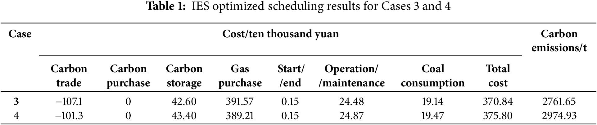
As shown in Table 1, compared to Case 4, Case 3 sees a 49,600-yuan reduction in IES operation cost. The gas purchase cost climbs by 23,600 yuan, while the coal consumption cost rises by just 3300 yuan. Operating in the hydrogen doping mode requires copious amounts of H2. Thus, to meet the demand, the electric load drives higher power output for H2 production, escalating overall power consumption. The IES chooses the lower-emission hydrogen-doped gas unit over the thermal unit, which hikes gas purchase costs but leaves coal costs nearly static. Between Case 3 and Case 4, carbon emissions declined by 213.28 t. Even though the hydrogen-doped gas turbine’s output in the IES increases, its per-unit electricity CO2 emission is lower. Thanks to the strong thermoelectric coupling and fixed thermal load, the hydrogen-doped gas turbine’s thermal output rises, the gas boiler’s thermal output drops, and the gas boiler emits less CO2 per unit of power.

5.3.2 Analysis of Hydrogen Doping Ratio Effectiveness

To further investigate the hydrogen doping ratio benefits, in this section, the hydrogen doping ratios were varied by changing the hydrogen doping ratio for gas turbines (HDR-GT) and gas boilers (HDR-GB) by setting the hydrogen doping ratios to 2%, 6%, 10%, 12%, and 16%, respectively. The hydrogen doping ratios were set to 2%, 6%, 10%, 12% and 16%, respectively. The relationship between CO2 emission and the total cost of IES for gas turbines and gas boilers with different hydrogen doping ratios is shown in Fig. 5.

Figure 5: Relationship between the total cost of IES and CO2 emission for different hydrogen doping ratios

As shown in Fig. 5a, when HDR-GT is fixed at 20% and HDR-GB at 16% and 2%, the IES’s total operating cost drops by 1%. With fixed HDR-GT, a rising HDR-GB leads to a decreasing cost of IES. When HDR-GB is fixed, increasing HDR-GT also reduces the IES cost, which levels off upon reaching 20%. In Fig. 5b, IES carbon emissions decline with growing HDR-GT, stabilizing at 18% or above. At HDR-GT of 15% and up, differences in emissions under various HDR-GB values shrink. Overall, the gas hydrogen doping mode cuts IES operation costs and emissions, enabling low-carbon operation. Properly setting HDR-GT and HDR-GB ratios can control these factors effectively.

5.3.3 Analysis of the Effectiveness of Variable Hydrogen Doping Ratios

Due to the electric-hydrogen strong coupling of EL (analogous to the gas turbine electric-thermal coupling), EL is forced to electrolyze H2 to satisfy the demand of H2 in the hydrogen doping mode, which generates a waste of electric energy. In this section, a comparative analysis of varying hydrogen doping ratios and fixed hydrogen doping ratios is used, and Case 5 is set as the variable hydrogen doping ratio mode. The hydrogen doping ratios of the gas turbine and gas boiler are shown in Fig. 6a, and the relationship between the unit’s hydrogen consumption power and net electric load in the two hydrogen doping modes is shown in Fig. 6b, and the results of IES optimal scheduling for Cases 3 and 5 are shown in Table 2.

Figure 6: Relationship between IES hydrogen consumption power and net electrical load in two hydrogen doping modes

As illustrated in Fig. 6, the hydrogen power consumption in the variable doping ratio mode is equivalent to or lower than the hydrogen power consumption in the fixed doping ratio mode. Furthermore, the hydrogen power consumption in the variable doping ratio mode exhibits a substantial decrease during the peak net electricity load period. As demonstrated in Table 3, in comparison with Case 3, Case 5 results in a reduction of the purchased gas cost by 7.15 ten thousand yuan. Despite an increase in carbon trading costs of 4.61 ten thousand yuan, the total cost is reduced by 3.75 ten thousand yuan, accompanied by a decrease in carbon emissions of 46.94 t. In summary, the IES modifies the power output of the gas turbine and the gas boiler by decreasing the amount of hydrogen doping, thereby reducing both the total cost and the carbon emission.

5.4 Analysis of the Effectiveness of CSP Plants

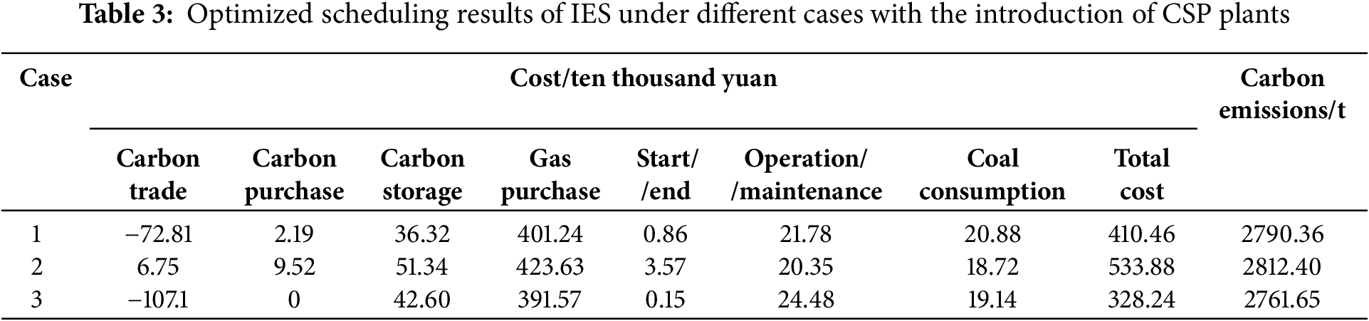
To verify the effectiveness of this paper’s IES introducing CSP plant, based on Case 3 in Section 4.2, this section sets three cases for comparative analysis: (1) using equal capacity PV units to replace the CSP plant to participate in the IES operation; (2) using the gas turbine with the same upper output limit and climbing power to replace the CSP plant to participate in the IES operation; and (3) the cases proposed in this paper. The results of IES optimal scheduling for the three cases are shown in Table 3.

As Table 3 shows, Case 3’s total cost drops by 19.64% compared to Case 1 and 38.52% against Case 2, proving the CSP plant’s good economic impact on IES optimal operation. Comparing Case 3 with Case 2, the carbon trading cost falls by 113.85 × 104 yuan, but the gas purchase cost rises by 32.06 × 104 yuan. Since the gas turbine, replacing the CSP plant, has a “thermal to set electricity” constraint, during electricity-heat load mismatches, it must increase output, hiking gas and carbon trading costs. Case 1, Case 3 uses PV units instead of CSP plants. Without sunlight, PV units need external gas and coal, raising gas turbine and thermal unit outputs. Case 3’s O&M cost is 12.40% higher than Case 1’s because CSP plant O&M involves thermal storage and power generation, so its unit power O&M cost is greater.

5.5 Sensitivity Analysis of Carbon Trading Mechanisms

In the Integrated Energy System (IES), the differences in stepped carbon trading parameters directly and significantly affect IES dispatching results. The carbon trading base price is a key parameter for in-depth study. In this research’s scheduling model, the amount of carbon emission allowances is much higher than the system’s actual emissions. As Fig. 7 shows, when the carbon trading base price is below 90 RMB, the system’s carbon emissions steadily decrease as the base price rises. This is because a higher base price strongly motivates the system to cut carbon emissions, enabling it to get more tradeable allowances and gain extra economic benefits. However, when the base price exceeds 90 RMB, the system’s carbon emissions stabilize, with few further fluctuations.

Figure 7: Sensitivity of carbon trading mechanisms to carbon trading base prices

Secondly, we consider the sensitivity of the carbon trading mechanism to the growth rate of the carbon trading price. With a baseline carbon trading base price of 90 yuan, as shown in Fig. 8, when the growth rate of the carbon trading price is in the range of [0, 0.2), carbon emissions show a downward trend. This is because a higher growth rate provides stronger incentives for the system to cut emissions, prompting a change in the unit output pattern and thus reducing carbon emissions. Fewer emissions mean the system can supply more carbon allowances, boosting revenue and cutting total costs. However, when the carbon trading price growth rate exceeds 0.2, the system’s ability to affect each unit’s output is nearly zero, and carbon emissions remain unchanged.

Figure 8: Sensitivity of carbon trading mechanisms to the magnitude of carbon trading price increases

It’s also remarkable that the total cost of the IES declines even as the carbon trading price goes up. To show how the carbon base price and its growth rate jointly affect the system’s carbon emissions, look at Fig. 9. Generally, a lower carbon base price along with a smaller increment in the carbon price correlates with higher overall carbon emissions in the system. Specifically, when the carbon trading base price is between 40 yuan and 120 yuan, the system displays different levels of sensitivity to various increases in the carbon trading price. However, once the carbon trading base price exceeds 120 yuan, changes in the carbon trading price no longer have an impact on the system’s carbon emissions.

Figure 9: Carbon emissions under varying carbon trading base prices and increments in carbon trading prices

5.6 Analysis of Fuzzy Affiliation Parameters

The selection of fuzzy affiliation parameters will have an impact on the optimal operation of IES. To study the impact of wind power output and load uncertainty on the total cost and carbon emission of IES, based on Case 3, set the confidence level as 0.98, and select different fuzzy affiliation parameter schemes shown in Table 4 for comparative validation, in which fuzzy degree 1 is the deterministic case, and get the relationship curves of the total cost and carbon emission of IES under the different fuzzy affiliation parameter shown in Fig. 7.

As can be seen in Fig. 10, with the same confidence level, the total IES cost, and carbon emissions increase as the level of ambiguity increases. Cases 2, 3, and 4 increase the total IES cost by 46.58%, 71.21%, and 82.10%, and the carbon emission by 19.13%, 25.29%, and 27.46%, respectively, compared to Case 1. The reason is that as the degree of ambiguity increases, the uncertainty of IES source load increases and faces higher operational risks, IES chooses to increase the purchased gas cost and gas unit output to cope with the risks, and the carbon emissions increase accordingly. Among them, the growth rate of carbon emissions is gradually smaller than the growth rate of the total cost of IES, because, under the CET mechanism, the price of carbon emission rights increases more and more, the cost of purchasing carbon emission allowances gradually increases, and IES chooses to purchase gas to cope with the risk of uncertainty.

Figure 10: Relationship between the total cost of IES and carbon emissions under different fuzzy affiliation parameters

5.7 Analysis of Weighting Factors

The CVaR weighting coefficients reflect the decision maker’s level of risk aversion caused by the uncertainty faced by the IES. To study the impact caused by the weighting coefficients on the optimal operation of IES, the CVaR confidence level is set to 0.98 based on Case 3 in Section 4.2, and the relationship curves between the total cost of IES and CVaR under different weighting coefficients are obtained as shown in Fig. 11:

Figure 11: Relationship curves of IES total cost and CVaR with different weighting coefficients

As shown in Fig. 11, the total IES cost and CVaR are 369.12 ten thousand yuan and 455.3 ten thousand yuan at φ=1.0, and 357.96 ten thousand yuan and 58.1 ten thousand yuan at φ=0.1, which is a decrease of 3.02% and an increase of 27.6%, respectively. As the weighting coefficient φ increases, the total cost of IES increases and CVaR decreases, and the larger the weighting coefficient, the larger the growth rate of the total cost of IES. The reason is that the larger the weight coefficient φ is, the more risk averse the decision maker is, and he chooses to increase the operation cost to avoid the risk; the smaller the weight coefficient φ is, the more risk-tolerant the decision maker is, and he chooses to take the risk to get the lower cost to guarantee the operation economics.

6  Conclusion

In this paper, in the background of IES containing a high proportion of renewable energy, CSP station is introduced in IES as renewable energy generation and storage, and the uncertainty analysis of renewable energy generation and load is carried out; gas hydrogen doping model is introduced on the basis of CCS-P2G coupled model, and carbon trading sensitivity analysis is carried out in combination with the stepped carbon trading mechanism, and the comparative study in different cases is conducted to get the following conclusions:

1.    The coupled CCS-P2G model with gas hydrogen doping unit reduces 1.32% operating cost and 7.17% carbon emission of IES and improves 5.73% carbon benefit.

2.    The variable hydrogen doping ratio model of EL reduces 3.75% operating cost and 1.70% carbon emission of IES and realizes the decoupling of EL electric-hydrogen strong coupling.

3.    CSP station involved in IES optimized operation reduced IES operating costs by 19.64% and 38.52%, and IES carbon emissions by 1.03% and 1.80%, respectively, compared with equivalent capacity PV and wind turbines.

4.    Sensitivity analysis of the carbon trading base price and its growth rate is carried out. When the base price is lower than 90 yuan, the carbon emission of IES decreases as the price rises, and when the base price is higher than 90 yuan, the carbon emission of IES tends to stabilize. When the price growth rate is in the interval of [0, 0.2], the carbon emission of IES decreases; when the price growth rate is in the interval of (0.2,+∞), the carbon emission of IES tends to stabilize.

5.    The carbon trading base price and its growth rate together affect the IES carbon emissions. The lower the base price is, the lower the price growth rate is, and the higher the IES carbon emissions are; when the base price is in the range of [40, 120], the IES shows different sensitivities to the price growth rate; when the base price is more than $120, the price growth rate has no impact on the IES carbon emissions.

6.    The sum of changes in the fuzzy affiliation parameter r1 for wind and load of 0.2, 0.25 and 0.3 increased the IES operating costs by 46.58%, 71.21% and 82.10% and the IES carbon emissions by 19.13%, 25.29% and 27.46%, respectively.

7.    The confidence level is fixed at 0.98 and the weighting coefficient φ is reduced from 1.0 to 0.1 in steps of 0.1, which reduces the IES operating cost by 3.02% and increases the CVaR cost by 27.6%. Decision makers need to make a balance among the weighting factor, total cost and CVaR, and select the optimal weighting factor to rationally avoid the risk by minimizing the cost.

This study has limitations in IES scheduling optimization. Currently, it relies only on forecast data, ignoring complex real-time power system conditions and intraday scheduling. In the future, adding an intraday rolling optimization scheduling link will enable the plan to adapt to real-time data, meeting IES optimization needs across time scales and following power system dynamics.

Acknowledgement: This research was supported by the State Grid Gansu Electric Power Company Science and Technology Program and the National Natural Science Foundation of China.

Funding Statement: State Grid Gansu Electric Power Company Science and Technology Program (Grant No. W24FZ2730008). National Natural Science Foundation of China (Grant No. 51767017).

Author Contributions: The authors confirm contribution to the paper as follows: Zhihui Feng: Funding acquisition, Resources; Jun Zhang: Data curation; Jun Lu: Project administration; Zhongdan Zhang: Data curation, Investigation; Wangwang Bai: Conceptualization; Long Ma: Formal analysis; Resources; Haonan Lu: Software, Visualization, Original draft; Jie Lin: Supervision, Writing—review and editing. All authors reviewed the results and approved the final version of the manuscript.

Availability of Data and Materials: The authors confirm that the data supporting the findings of this study are available within the article.

Ethics Approval: This study is theoretical in nature and does not involve human or animal experimentation or the collection of personal data, and therefore does not require the approval of an ethics committee.

Conflicts of Interest: The authors declare no conflicts of interest to report regarding the present study.

Nomenclature

Appendix A

Eq. (31) contains the square term, for which the segmented linearization method is used in the following procedure:

Step 1: Take M+1 segmentation points [l1,l2,⋯,lM+1] and divide the original equation into M intervals.

Step 2: Add M+1 continuous auxiliary variable [r1,r2,⋯,rM+1], M binary auxiliary variable [k1,k2,⋯,kM]:

{r1+r2+⋯+rM+1=1k1+k2+⋯+kM=1r1≥0,r2≥0,⋯,rM+1≥0r1≤k1,r2≤k1+k2,⋯,rM+1≤kM(A1)

Step 3: Replace the nonlinear expression with Eq. (A2):

{Ptth=∑m=1M+1rmlmfth=∑m=1M+1rmfth(lm)(A2)

For Eq. (25), linearization is performed using steps 2 and 3.

Appendix B

Figure A1: IES Forecasts for electric thermal load, wind power and DNI

Figure A2: CO2 power diagram for IES

References

1. Zhang W, Xu Y. Distributed optimal control for multiple microgrids in a distribution network. IEEE Trans Smart Grid. 2019;10(4):3765–79. doi:10.1109/TSG.2018.2834921. [Google Scholar] [CrossRef]

2. Zhang SX, Wang DY, Yang HZ, Song Y, Yuan K, Du W. Key technologies and challenges of low-carbon integrated energy system planning for carbon emission peak and carbon neutrality. Autom Electr Power Syst. 2022;46(8):189–207 (In Chinese). [Google Scholar]

3. Fu X, Zhang X, Qiao Z, Li G. Estimating the failure probability in an integrated energy system considering correlations among failure patterns. Energy. 2019;178(2):656–66. doi:10.1016/j.energy.2019.04.176. [Google Scholar] [CrossRef]

4. Zhang G, Wang W, Chen Z, Li R, Niu Y. Modeling and optimal dispatch of a carbon-cycle integrated energy system for low-carbon and economic operation. Energy. 2022;240:122795. doi:10.1016/j.energy.2021.122795. [Google Scholar] [CrossRef]

5. Chen YB, Zhang N, Li JQ, Fang Z, Wu SC, Mei SW, et al. Review and prospect of zero carbon park research. Proc CSEE. 2024;44(14) (In Chinese). doi:10.13334/j.0258-8013.pcsee.231293. [Google Scholar] [CrossRef]

6. Wang R, Wen X, Wang X, Fu Y, Zhang Y. Low carbon optimal operation of integrated energy system based on carbon capture technology, LCA carbon emissions and ladder-type carbon trading. Appl Energy. 2022;311(7):118664. doi:10.1016/j.apenergy.2022.118664. [Google Scholar] [CrossRef]

7. Zhu H, Yu T, Chen Z, Wu Y, Li Z, Wu W. Distributed optimal dispatching of interconnected electricity-gas-heating system. IEEE Access. 2020;8:93309–21. doi:10.1109/ACCESS.2020.2994771. [Google Scholar] [CrossRef]

8. Zhou RJ, Xiao JW, Tang XF, Zheng QG, Lv J, Cao JB. Coordinated optimization of carbon utilization between power-to-gas renewable energy accommodation and carbon capture power plant. Electr Power Autom Equip. 2018;38(7):61–7 (In Chinese). doi:10.16081/j.issn.1006-6047.2018.07.008. [Google Scholar] [CrossRef]

9. Zhou RJ, Deng ZA, Xu J, Zhu JS, Wang YZ. Optimized operation using carbon recycling for benefit of virtual power plant with carbon capture and gas thermal power. Electr Power. 2020;53(9):166–71 (In Chinese). doi:10.11930/j.issn.1004-9649.201908007. [Google Scholar] [CrossRef]

10. Sun HJ, Liu Y, Peng CH, Meng JH. Optimization scheduling of virtual power plant with carbon capture and waste incineration considering power-to-gas coordination. Power Syst Technol. 2021;45(9):3534–45 (In Chinese). doi:10.13335/j.1000-3673.pst.2020.1720. [Google Scholar] [CrossRef]

11. Zhang XP, Zhang YZ. Multi-objective optimization model for park-level electricity-heat-gas integrated energy system considering P2G and CCS. Electr Power Constr. 2020;41(12):92–101 (In Chinese). doi:10.12204/j.issn.1000-7229.2020.12.009. [Google Scholar] [CrossRef]

12. Chen BD, Lin KD, Zhang YJ, Chen ZX, Wang J, Su JY. Optimal dispatching of integrated electricity and natural gas energy systems considering the coordination of carbon capture system and power-to-gas. South Power Syst Technol. 2019;13(11):9–17 (In Chinese). doi:10.13648/j.cnki.issn1674-0629.2019.11.002. [Google Scholar] [CrossRef]

13. Tian F, Jia YB, Ren HQ, Bai Y, Huang T. “Source-load” low-carbon economic dispatch of integrated energy system considering carbon capture system. Power Syst Technol. 2020;44(9):3346–55 (In Chinese). doi:10.13335/j.1000-3673.pst.2020.0728. [Google Scholar] [CrossRef]

14. Peng Y, Lou SH, Wu YW, Wang Y, Zhou KP. Low-carbon economic dispatch of power system with wind power considering solvent-storaged carbon capture power plant. Trans China Electrotech Soc. 2021;36(21):4508–16 (In Chinese). doi:10.19595/j.cnki.1000-6753.tces.201249. [Google Scholar] [CrossRef]

15. Zhou RJ, Sun H, Tang XF, Zhang WJ, Yu H. Low-carbon economic dispatch based on virtual power plant made up of carbon capture unit and wind power under double carbon constraint. Proc CSEE. 2018;38(6):1675–83,1904 (In Chinese). doi:10.13334/j.0258-8013.pcsee.170541. [Google Scholar] [CrossRef]

16. Chen HP, Chen JD, Zhang Z, Wang CL, Wang JQ, Han H, et al. Low-carbon economic dispatching of power system considering capture energy consumption of carbon capture power plants with flexible operation mode. Electr Power Autom Equip. 2021;41(9):133–9 (In Chinese). doi:10.16081/j.epae.202109040. [Google Scholar] [CrossRef]

17. Ma Y, Wang H, Hong F, Yang J, Chen Z, Cui H, et al. Modeling and optimization of combined heat and power with power-to-gas and carbon capture system in integrated energy system. Energy. 2021;236(5):121392. doi:10.1016/j.energy.2021.121392. [Google Scholar] [CrossRef]

18. Wang S, Wang S, Zhao Q, Dong S, Li H. Optimal dispatch of integrated energy station considering carbon capture and hydrogen demand. Energy. 2023;269(1):126981. doi:10.1016/j.energy.2023.126981. [Google Scholar] [CrossRef]

19. Jin J, Wen Q, Cheng S, Qiu Y, Zhang X, Guo X. Optimization of carbon emission reduction paths in the low-carbon power dispatching process. Renew Energy. 2022;188(12):425–36. doi:10.1016/j.renene.2022.02.054. [Google Scholar] [CrossRef]

20. Sun Q, Wang X, Liu Z, Mirsaeidi S, He J, Pei W. Multi-agent energy management optimization for integrated energy systems under the energy and carbon co-trading market. Appl Energy. 2022;324(5):119646. doi:10.1016/j.apenergy.2022.119646. [Google Scholar] [CrossRef]

21. Liu D, Luo Z, Qin J, Wang H, Wang G, Li Z, et al. Low-carbon dispatch of multi-district integrated energy systems considering carbon emission trading and green certificate trading. Renew Energy. 2023;218:119312. doi:10.1016/j.renene.2023.119312. [Google Scholar] [CrossRef]

22. Yang M, Liu Y. Research on multi-energy collaborative operation optimization of integrated energy system considering carbon trading and demand response. Energy. 2023;283:129117. doi:10.1016/j.energy.2023.129117. [Google Scholar] [CrossRef]

23. Aseri TK, Sharma C, Kandpal TC. A techno-economic appraisal of parabolic trough collector and central tower receiver based solar thermal power plants in India: effect of nominal capacity and hours of thermal energy storage. J Energy Storage. 2022;48:103976. doi:10.1016/j.est.2022.103976. [Google Scholar] [CrossRef]

24. Praveen RP, Chandra Mouli KVV. Performance enhancement of parabolic trough collector solar thermal power plants with thermal energy storage capability. Ain Shams Eng J. 2022;13(5):101716. doi:10.1016/j.asej.2022.101716. [Google Scholar] [CrossRef]

25. Wei S, Liang X, Mohsin T, Wu X, Li Y. A simplified dynamic model of integrated parabolic trough concentrating solar power plants: modeling and validation. Appl Therm Eng. 2020; 169:114982. doi:10.1016/j.applthermaleng.2020.114982. [Google Scholar] [CrossRef]

26. Cui Y, Yu S, Wang X, Fu G, Wang M. Optimal configuration of heat storage capacity considering the balance between system peak shaving demand and concentrating solar power plant revenue. Proc of the CSEE. 2023; 43(228745–56. [Google Scholar]

27. Wang Y, Lou S, Wu Y, Wang S. Co-allocation of solar field and thermal energy storage for CSP plants in wind-integrated power system. IET Renew Power Gener. 2018; 12(14):1668–74. doi:10.1049/iet-rpg.2018.5224. [Google Scholar] [CrossRef]

28. Du E, Zhang N, Hodge BM, Wang Q, Kang C, Kroposki B, et al. The role of concentrating solar power toward high renewable energy penetrated power systems. IEEE Trans Power Syst. 2018;33(6):6630–41. doi:10.1109/TPWRS.2018.2834461. [Google Scholar] [CrossRef]

29. Chen R, Sun H, Guo Q, Li Z, Deng T, Wu W, et al. Reducing generation uncertainty by integrating CSP with wind power: an adaptive robust optimization-based analysis. IEEE Trans Sustain Energy. 2015;6(2):583–94. doi:10.1109/TSTE.2015.2396971. [Google Scholar] [CrossRef]

30. Du E, Zhang N, Hodge BM, Kang C, Kroposki B, Xia Q. Economic justification of concentrating solar power in high renewable energy penetrated power systems. Appl Energy. 2018;222(2):649–61. doi:10.1016/j.apenergy.2018.03.161. [Google Scholar] [CrossRef]

31. Jorgenson J, Denholm P, Mehos M. Estimating the value of utility-scale solar technologies in California under a 40% renewable portfolio standard. Golden CO: National Renewable Energy Laboratory; 2014. [Google Scholar]

32. Guevara E, Babonneau F, Homem-de-Mello T, Moret S. A machine learning and distributionally robust optimization framework for strategic energy planning under uncertainty. Appl Energy. 2020;271(2):115005. doi:10.1016/j.apenergy.2020.115005. [Google Scholar] [CrossRef]

33. Chen Y, Chen C, Ma J, Qiu W, Liu S, Lin Z, et al. Multi-objective optimization strategy of multi-sources power system operation based on fuzzy chance constraint programming and improved analytic hierarchy process. Energy Rep. 2021;7(5):268–74. doi:10.1016/j.egyr.2021.01.070. [Google Scholar] [CrossRef]

34. Li GQ, Li XT, Bian J, Li ZH. Two level scheduling strategy for inter-provincial DC power grid considering the uncertainty of PV-load prediction. Proc CSEE. 2021;41(14):4763–76 (In Chinese). doi:10.13334/j.0258-8013.pcsee.200763. [Google Scholar] [CrossRef]

35. Chen JM, Xu Q, Li Y, Yu XW, Chen WC. Optimal dispatch of electricity-natural gas interconnection system considering source-load uncertainty and virtual power plant with carbon capture. Acta Energiae Solaris Sin. 2023;44(10):9–18 (In Chinese). doi:10.19912/j.0254-0096.tynxb.2022-0840. [Google Scholar] [CrossRef]

36. Salehi J, Namvar A, Gazijahani FS. Scenario-based Co-Optimization of neighboring multi carrier smart buildings under demand response exchange. J Clean Prod. 2019;235(4):1483–98. doi:10.1016/j.jclepro.2019.07.068. [Google Scholar] [CrossRef]

37. Yao JM, Zhao SQ, Wei ZY, Zhang H. Day-ahead dispatch and its fast solution method of power system based on scenario analysis. Electr Power Autom Equip. 2022;42(9):102–10 (In Chinese). doi:10.16081/j.epae.202204022. [Google Scholar] [CrossRef]

38. Lü HP, Xiwang A, Meng LP. Two-stage stochastic optimal scheduling of microgrid considering uncertainty of source-load forecasting. Electr Power Autom Equip. 2022;42(9):70–8 (In Chinese). [Google Scholar]

39. Zhang M, Wang JH, Chang X, Yang CY, Li R, Sun CW, et al. Multi-objective robust planning method for heat-electricity coupled micro energy system considering uncertainty of renewable energy. Electric Power China. 2021;54(4):119–129, 140 (In Chinese). [Google Scholar]

40. Lei D, Zhang Z, Wang Z, Zhang L, Liao W. Long-term, multi-stage low-carbon planning model of electricity-gas-heat integrated energy system considering ladder-type carbon trading mechanism and CCS. Energy. 2023;280(9):128113. doi:10.1016/j.energy.2023.128113. [Google Scholar] [CrossRef]

41. Chen M, Lu H, Chang X, Liao H. An optimization on an integrated energy system of combined heat and power, carbon capture system and power to gas by considering flexible load. Energy. 2023;273(4):127203. doi:10.1016/j.energy.2023.127203. [Google Scholar] [CrossRef]

42. He L, Lu Z, Zhang J, Geng L, Zhao H, Li X. Low-carbon economic dispatch for electricity and natural gas systems considering carbon capture systems and power-to-gas. Appl Energy. 2018;224(4):357–70. doi:10.1016/j.apenergy.2018.04.119. [Google Scholar] [CrossRef]