
 Submit a Paper
 Propose a Special lssue
 Open Access
ARTICLE

Short-Term Prediction of Photovoltaic Power Based on Improved CNN-LSTM and Cascading Learning
The College of Engineering, Shanghai Ocean University, Shanghai, 201306, China
* Corresponding Author: Chen Yang. Email:
(This article belongs to the Special Issue: Modelling, Optimisation and Forecasting of Photovoltaic and Photovoltaic thermal System Energy Production)
Energy Engineering 2025, 122(5), 1975-1999. https://doi.org/10.32604/ee.2025.062035
Received 09 December 2024; Accepted 17 March 2025; Issue published 25 April 2025
 View Full Text
 Download PDF
Abstract
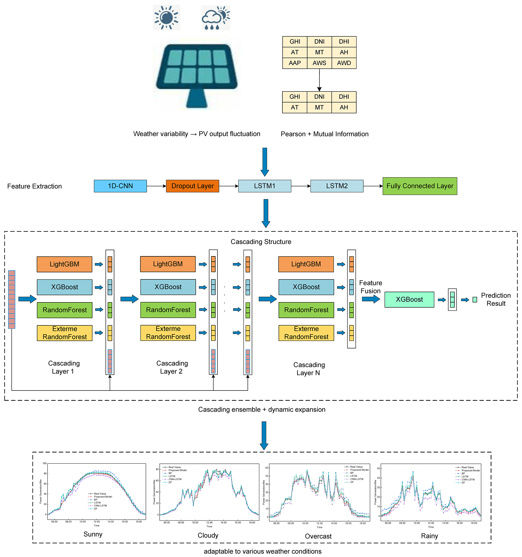
Short-term photovoltaic (PV) power forecasting plays a crucial role in enhancing the stability and reliability of power grid scheduling. To address the challenges posed by complex environmental variables and difficulties in modeling temporal features in PV power prediction, a short-term PV power forecasting method based on an improved CNN-LSTM and cascade learning strategy is proposed. First, Pearson correlation coefficients and mutual information are used to select representative features, reducing the impact of redundant features on model performance. Then, the CNN-LSTM network is designed to extract local features using CNN and learn temporal dependencies through LSTM, thereby obtaining feature representations rich in temporal information. Subsequently, a multi-layer cascade structure is developed, progressively integrating prediction results from base learners such as LightGBM, XGBoost, Random Forest (RF), and Extreme Random Forest (ERF) to enhance model performance. Finally, an XGBoost-based meta-learner is utilized to integrate the outputs of the base learners and generate the final prediction results. The entire cascading process adopts a dynamic expansion strategy, where the decision to add new cascade layers is based on the R2 performance criterion. Experimental results demonstrate that the proposed model achieves high prediction accuracy and robustness under various weather conditions, showing significant improvements over traditional models and providing an effective solution for short-term PV power forecasting.Graphic Abstract
Keywords
With the transformation of China’s energy system and the implementation of the “dual carbon” goal, power generation technologies dominated by renewable energy have developed rapidly, making photovoltaic (PV) power generation an increasingly important method of renewable energy generation in China [1]. The output power of PV generation is significantly affected by meteorological conditions (such as irradiance, temperature, and humidity) and fluctuates drastically under extreme weather conditions. This leads to unstable PV power supply, posing challenges for optimized power system scheduling and the safe operation of power grids [2–4]. Therefore, accurate PV power forecasting is crucial for improving energy utilization efficiency, system stability, and energy supply security in power systems [5].
To effectively address the uncertainties in PV power generation, various forecasting methods have been proposed in recent years, which can be broadly divided into physical models [6], statistical models [7], and machine learning-based models [8]. Physical models primarily rely on measurements of environmental parameters such as solar irradiance, temperature, and humidity, as well as the modeling of the physical characteristics of PV modules. Mayer et al. [9] demonstrated that although physical models can effectively leverage solar radiation and other environmental parameters by incorporating physical characteristics, their reliance on precise measurement limits their practical application. Statistical models, such as time series analysis methods like ARIMA [10], forecast power output by modeling the power time series data. These models can capture power output trends effectively, but they struggle to achieve high accuracy under complex environmental conditions. In contrast, machine learning models, which have adaptive learning capabilities and can model complex data relationships, have gradually become a key approach in PV power forecasting. Studies have shown that machine learning models exhibit significant advantages in short-term PV forecasting, especially in dealing with non-linear models and complex feature data [11].
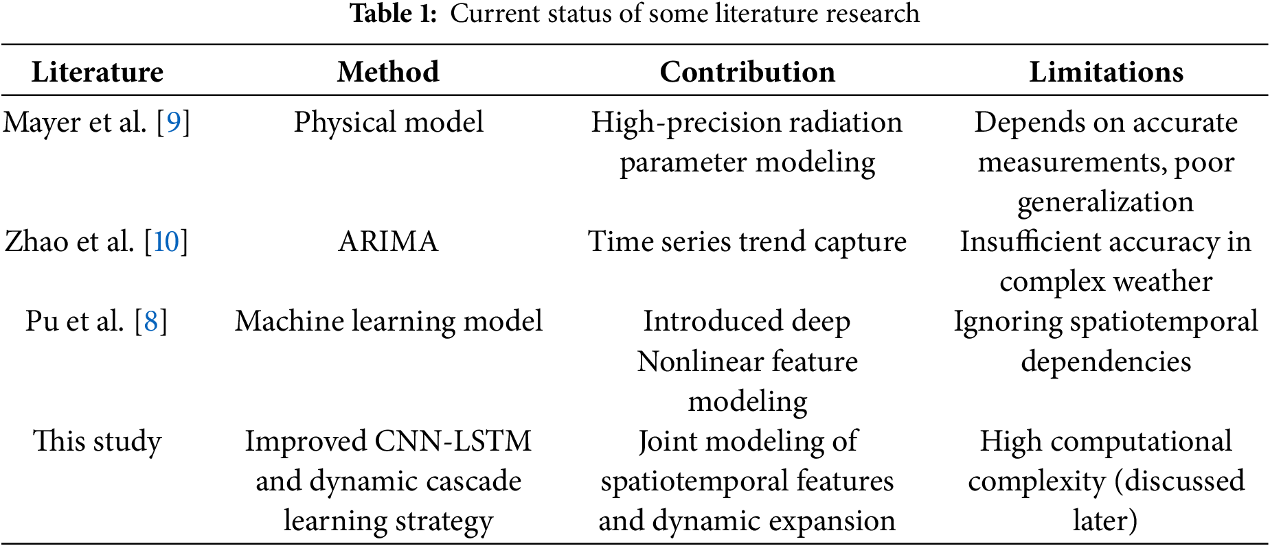
Deep learning has demonstrated outstanding capabilities in feature extraction and modeling, leading to breakthroughs in multiple fields. Specifically, Convolutional Neural Networks (CNN) and Long Short-Term Memory (LSTM) networks have demonstrated outstanding performance in tasks such as image recognition, natural language processing, and time series analysis [12]. Deep learning models can enhance accuracy and efficiency across various applications through automated feature extraction and modeling of complex patterns. Zhang et al. [13] illustrated how deep learning can improve model performance via automated feature extraction, while Hochreiter et al. [14] introduced the LSTM model, effectively addressing the vanishing gradient problem in long-sequence data. CNN excels at extracting local features from input data, while LSTM is effective at capturing long-term dependencies in time series. Wang et al. [15] further validated the performance of LSTM in power demand forecasting and other time series tasks, demonstrating its advantages in capturing long-term dependency features. These characteristics make the combination of CNN and LSTM highly promising for PV power forecasting. However, PV power forecasting involves not only complex environmental variables but also significant temporal features, requiring a model that can simultaneously capture both local characteristics and temporal dependencies, which poses higher demands on model design. Table 1 is added to compare the methods, contributions and limitations of existing studies to clarify the research innovations of this paper.
In summary, this paper proposes a PV power forecasting method based on an improved CNN-LSTM model combined with a cascading learning strategy, to tackle the challenges posed by complex environmental variables and time series modeling in PV power generation. First, feature selection is performed using Pearson correlation and mutual information to effectively reduce redundant features and improve the model’s generalization ability and robustness. Second, a CNN-LSTM model is employed, where CNN extracts local spatial features and LSTM captures temporal dependencies, generating feature representations with rich temporal information. Next, a multi-layer cascade structure is constructed, which integrates the predictions of various base learners, including LightGBM, XGBoost, RF, and ERF, in a stepwise manner to further enhance the model’s performance. Finally, XGBoost is used as the meta-learner to integrate the outputs of each cascade layer, and a dynamic extension strategy based on R2 value is applied to ensure optimal prediction performance under different environmental conditions. Experimental results indicate that the proposed method demonstrates high prediction accuracy and robustness under various weather conditions, reducing Mean Absolute Error (MAE) and Root Mean Square Error (RMSE) by 27.95% and 20.87%, respectively, compared with existing methods. The proposed study provides an effective technical solution for accurate PV power forecasting, with potential applications in power system scheduling optimization and grid safety management.
Photovoltaic (PV) power generation is primarily influenced by solar irradiance and temperature, while certain features indirectly affect PV power generation by influencing the temperature of PV modules and their exposure to solar radiation. As a result, there are multiple features that impact PV power generation. In this study, we perform a feature correlation analysis using monitoring data from a PV power plant in Shanghai, covering the period from 00:00 on 10 August 2023, to 00:00 on 10 August 2024. The plant has a total installed capacity of 110 MW, with data sampled at 15-min intervals, a total of 35,040 samples were generated throughout the year, containing nine features as GHI, DNI, DHI, AT, MT, AH, AAP, AWS, AWD. Among these, AWS and AWD are measured at a height of 10 m.
Due to various uncertainty factors in the real environment, PV data collection may result in missing or anomalous data. To ensure the completeness of the dataset, it is essential to identify and accurately repair anomalies in the raw PV data and effectively fill in the missing values. In this study, the Akima interpolation method is used to fill in missing data. The algorithm applies a weighted averaging principle, where the weight of each data point is determined based on the slope between adjacent data points. To handle anomalous data values, the Inter Quartile Range (IQR) method is employed. Anomalies are detected using box plots, and the anomalous values are then corrected by replacing them with the mean of the corresponding data group. The IQR is calculated for the dataset to identify any outliers.
2.2 Based on Pearson Correlation and Mutual Information for Feature Selection
The output power of photovoltaic (PV) systems is influenced by various environmental factors, including both linear and nonlinear factors. To improve the accuracy and stability of the model in PV power prediction, this study employs a feature selection method combining Pearson Correlation Coefficient (PCC) and Mutual Information (MI) [16,17]. This method selects the most relevant features from the input variables that are most strongly correlated with the target variable. This step helps reduce data redundancy and noise, ensuring that the final feature set input into the model has high informational value.
Assuming meteorological features are random variables
where
Mutual Information (MI) is a non-parametric statistic that measures the degree of information shared between two variables. It can capture both linear and nonlinear relationships. The mutual information can be defined as:
where
Assuming the PV dataset contains
The threshold for feature selection is then determined as:
Since these features not only exhibit significant linear correlations but are also closely related to the target variable in complex nonlinear patterns, we calculate both the Pearson correlation coefficient and the mutual information, and then take the intersection of the two results to determine the final feature set. The feature selection process is shown in Fig. 1.
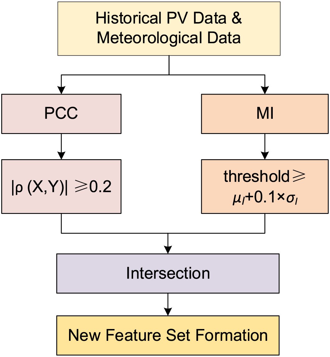
Figure 1: Feature selection process
This feature selection process ensures that the features input into the model not only have a significant linear relationship with the target variable but also capture more complex nonlinear associations, reducing the negative impact of noise and redundant features on model training. Table 2 shows the correlation coefficients and mutual information values between the meteorological features and PV power. As observed in Table 2, GHI exhibits both the highest correlations (PCC = 0.988 and MI = 1.652), confirming its dominant role in PV power prediction. DHI also demonstrates strong correlations (PCC = 0.922 and MI = 1.372), indicating its complementary relationship with GHI under varying sky conditions. Notably, AT and MT show moderate MI scores (0.184 and 0.199, respectively) despite relatively low PCC values (0.260 and 0.336), suggesting their nonlinear influences on PV power through thermal effects. The selected features exhibit clear interpretability:
(1) GHI/DNI/DHI collectively represent solar irradiance components, with GHI capturing 98.8% of linear variability.
(2) MT and AT reflect temperature-dependent efficiency degradation, where MI values reveal nonlinear thermal losses.
(3) AH shows an inverse linear correlation (PCC = −0.218) but significant MI (0.251), indicating humidity impacts PV power through condensation mechanisms beyond simple linear relationships.
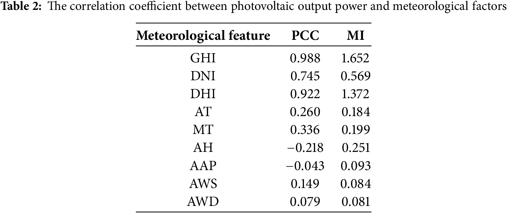
Conversely, features like AWS and AWD were excluded due to negligible correlations (PCC < 0.15, MI < 0.1), as their effects are secondary and localized. This dual-criterion selection (PCC∩MI) effectively eliminates redundant features (e.g., AAP with PCC = −0.043) while retaining physically meaningful variables. Following the above feature selection process using mutual information and Pearson correlation coefficients, we selected six features-GHI, DNI, DHI, AT, MT and AH-to predict PV power generation.
CNN are deep learning models based on weight sharing and local connectivity, which significantly reduce model complexity while still efficiently extracting deep feature information from data. A typical CNN consists of an input layer, convolutional layers, pooling layers, fully connected layers, and an output layer. The convolutional layers extract local features from the input data through convolution operations, while the pooling layers perform downsampling to further reduce the volume of data, thereby retaining key features and minimizing computational load [18]. This hierarchical feature extraction mechanism enables CNNs to achieve excellent performance in handling complex data. The structure of a one-dimensional CNN (1D-CNN) is illustrated in Fig. 2. In this study, a 1D-CNN is used to extract local feature patterns from meteorological sequences of PV power generation. The convolutional layers slide their kernels over the input sequence, learning local feature patterns of environmental variables, such as irradiance and temperature, over short time intervals.
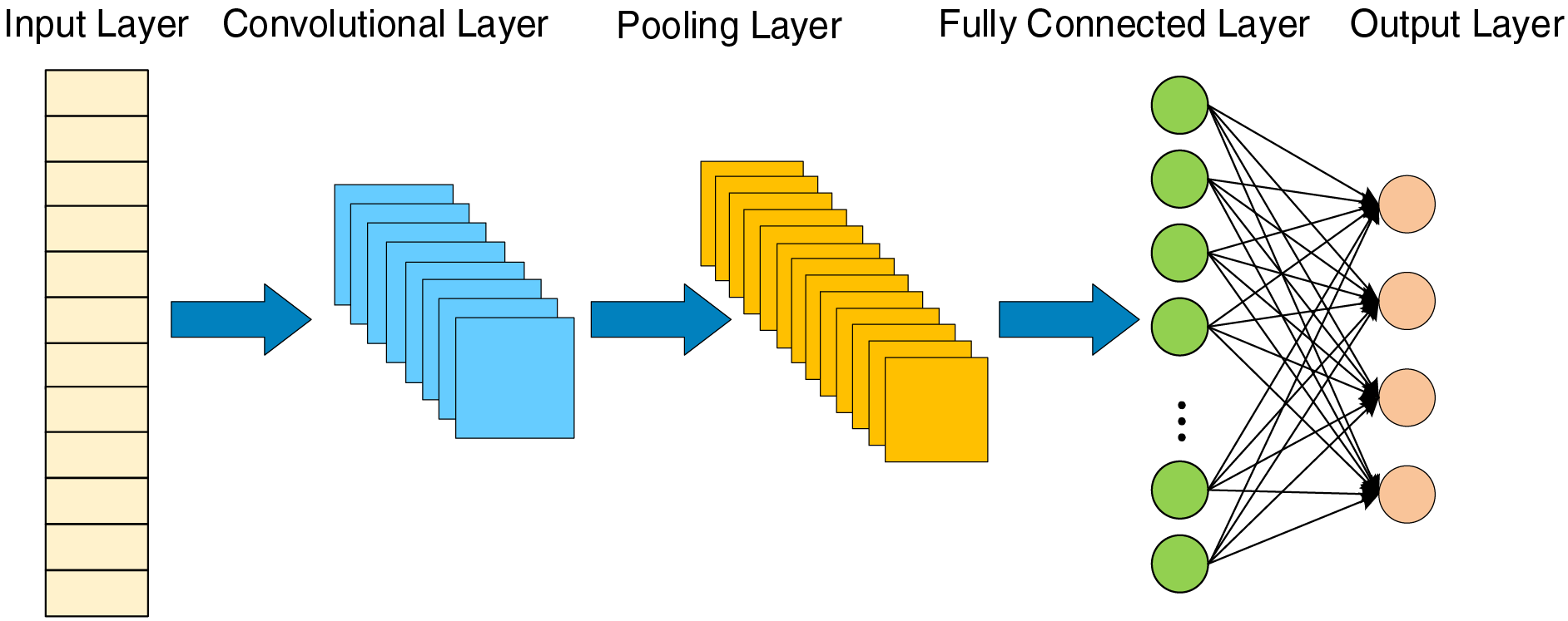
Figure 2: Structure diagram of 1D-CNN model
LSTM is a special type of Recurrent Neural Network (RNN) that adds three core gating units to the traditional RNN: the forget gate, the input gate, and the output gate. The forget gate is responsible for selectively retaining or discarding historical information, thus filtering the information flow. The input gate controls the update of the memory cell state based on the current input, while the output gate determines which information will influence the current output state. By incorporating these gating mechanisms and specialized memory cells, LSTM is capable of capturing long-term dependencies, which makes it particularly effective in handling long-term memory retention issues when processing time series data. The structure of LSTM is shown in Fig. 3.
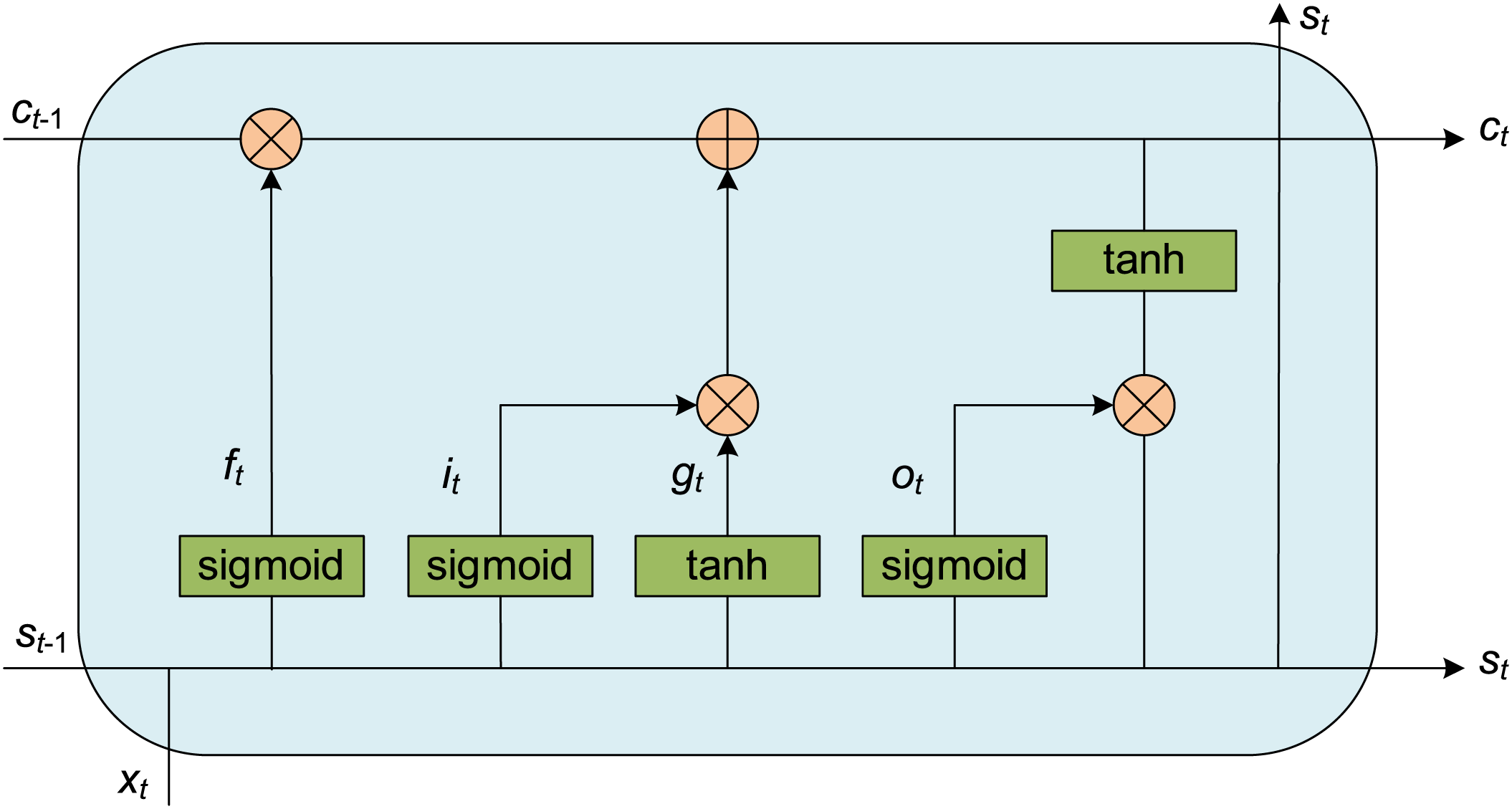
Figure 3: Structure diagram of LSTM
where
1D-CNN-LSTM is a hybrid neural network that combines the feature extraction capability of 1D-CNN with the long-term memory capability of LSTM for time series data [19]. In this study, the 1D-CNN-LSTM model is used to extract deep features from PV power generation data that have been preprocessed through feature selection and standardization, aiming to improve prediction performance. The specific model structure is shown in Fig. 4.
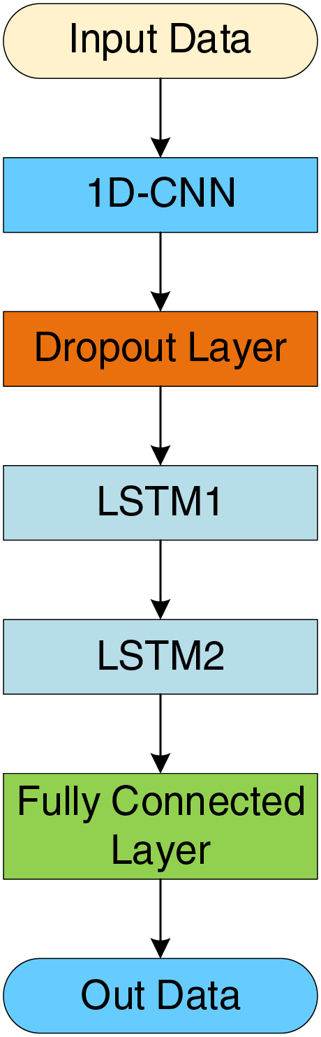
Figure 4: 1D-CNN-LSTM hybrid neural network model
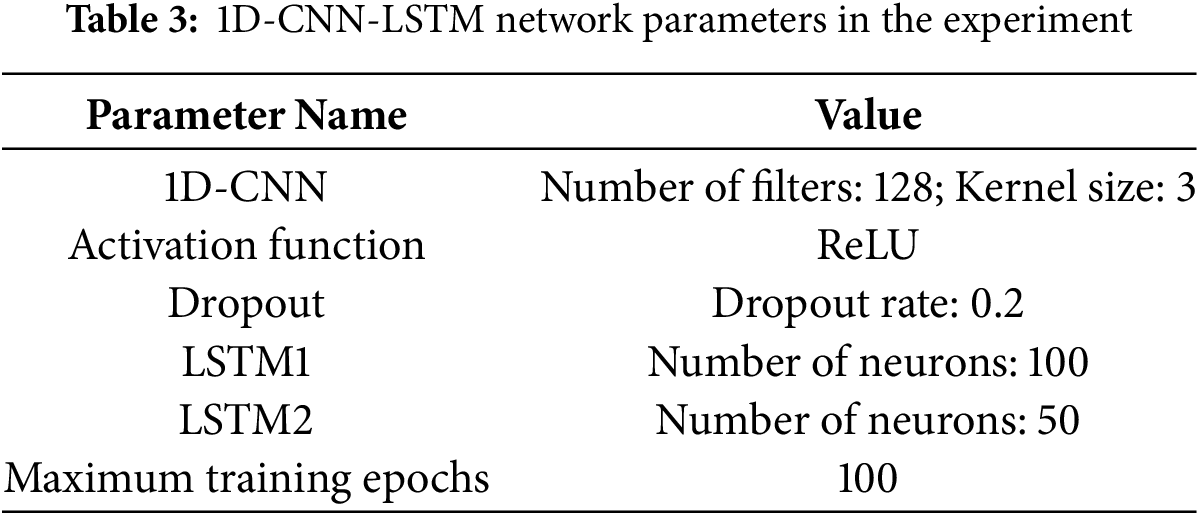
For the data input to the 1D-CNN-LSTM, the process begins with a one-dimensional convolutional layer that extracts local features from the input time series data, capturing spatial patterns in the data. The ReLU activation function is used in this step. Then, a Dropout layer is added to reduce the risk of overfitting. Next, two LSTM layers are employed, each learning the temporal dependencies of the data, effectively modeling both long-term and short-term variations in the time series, thereby improving the model’s understanding of the data. After the LSTM layers, the output is passed through a fully connected layer that maps the final features to the original feature dimensions, facilitating regression prediction. The grid search parameters used in the 1D-CNN-LSTM model during the experiment are shown in Table 3.
3.4 Stacking Ensemble Learning
Stacking ensemble learning is an ensemble machine learning method that combines the predictions from multiple base models to improve overall predictive performance [20]. Unlike traditional single models, Stacking aims to enhance accuracy by integrating various base models. Unlike conventional ensemble methods, the distinctive feature of Stacking lies in using a meta-learner to aggregate the outputs from multiple base learners, thus generating the final prediction. In a Stacking framework, base learners typically include different types of models, such as decision trees, linear regression, and support vector machines. Each base learner is trained separately on the training data to produce preliminary predictions, which are then used as new features and fed into a meta-learner for final learning. The meta-learner’s task is to make an optimal combination of the outputs from the base learners, thereby improving the prediction’s accuracy and robustness. The structure of the Stacking model is illustrated in Fig. 5.
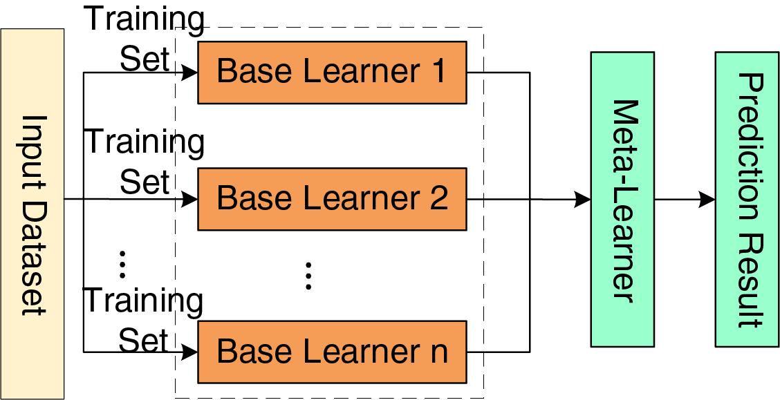
Figure 5: Structure diagram of stacking model
3.5 Introduction to Other Algorithms
Gradient Boosting Decision Tree (GBDT) improves the predictive performance of a model by iteratively training a series of decision trees. XGBoost is an ensemble learning algorithm [21] known for its high predictive accuracy, particularly when dealing with large-scale datasets. When processing tabular data, XGBoost often outperforms most deep neural network frameworks and traditional machine learning algorithms.
LightGBM is a lightweight gradient boosting model developed by Microsoft in 2017 [22]. Based on GBDT, LightGBM incorporates techniques such as Gradient-Based One-Side Sampling (GOSS), Exclusive Feature Bundling (EFB), histogram-based optimization, and a leaf-wise growth strategy with limited depth. These improvements make the model particularly suitable for handling large-scale datasets and high-dimensional feature tasks.
Random Forest (RF) is a machine learning model with strong generalization capabilities [23]. The core idea of RF is to construct multiple relatively independent decision tree models using the Bagging method, and then aggregate the predictions of these trees either by averaging (for regression tasks) or voting (for classification tasks) to obtain the final prediction.
GridSearchCV is a widely used optimization method for hyperparameter tuning in machine learning models [24]. Its primary goal is to systematically search a pre-defined hyperparameter space to find the combination of parameters that yields the best model performance, thus enhancing predictive accuracy. GridSearchCV combines exhaustive search and cross-validation by generating all possible parameter combinations and validating each combination on different subsets of the data to ensure model robustness. GridSearchCV first defines a hyperparameter grid space and then traverses all combinations through exhaustive search. Additionally, it uses a cross-validation mechanism, where the dataset is divided into multiple subsets to evaluate model performance, typically adopting k-fold cross-validation. In k-fold cross-validation, the dataset is randomly split into k mutually exclusive subsets. Each time,
4 Photovoltaic Power Prediction Model Based on Improved CNN-LSTM and Cascading Learning
To effectively address the complex environmental features and significant temporal characteristics inherent in photovoltaic (PV) power generation data, this paper proposes an improved PV power prediction model that integrates deep learning with ensemble learning. By combining deep feature extraction with multi-base learner cascading integration, the proposed model significantly enhances the accuracy of PV power predictions. The overall model is composed of three main modules: a 1D-CNN-LSTM feature extraction module, a cascading learning module, and a fusion layer module. The feature extraction module is used to capture both local and temporal features of environmental variables, the cascading learning module improves the overall expressive capability of the model, and the fusion layer is used to optimize the final output prediction. The structure of the PV power prediction model based on CNN-LSTM and cascading learning is shown in Fig. 6. The specific process is as follows:
(1) 1D-CNN-LSTM Feature Extraction
The traditional Deep Forest (DF) model relies on the feature combination approach of tree-based models [25], which lacks the ability to deeply extract intrinsic data features, especially in time series scenarios where it struggles to capture local feature patterns and temporal dependencies. Therefore, this study introduces 1D-CNN and LSTM as the feature extraction module to enhance the expressiveness of time series features.

Figure 6: Structure diagram of photovoltaic power prediction model based on CNN-LSTM and cascading learning
First, 1D-CNN is used to extract local features from the meteorological sequences of PV power generation. The convolutional layer slides its kernels over the input sequence to learn short-term local patterns of environmental variables (e.g., irradiance, temperature). This convolutional operation effectively extracts short-term correlations among environmental features, generating local feature representations. Next, LSTM is applied to the extracted local features for further temporal modeling, capturing long-term dependencies. The multi-layer LSTM design enables the model to capture not only short-term variations but also long-term trends effectively. This improvement ensures that the model retains local features while fully leveraging the temporal dependencies within sequential data, thereby enhancing its performance in handling time series data.
(2) Cascading Layer Design and Dynamic Expansion Strategy
In the Deep Forest model, feature extraction and classification/regression are achieved through a multi-layer cascading structure. Traditional Deep Forest models usually employ Random Forest (RF) and Extreme Random Forest (ERF) as base learners to facilitate feature combination and enhancement. However, a single type of base learner may not be sufficient to fully capture the complexities of the data. Therefore, this study proposes a multi-model cascading structure, incorporating multiple types of base learners, including LightGBM, XGBoost, RF, and ERF, thereby enhancing the model’s expressive power and generalization ability.
In each cascading layer, these base learners are used to model the input features, and the prediction results from each base learner are combined with the original features
where
To further enhance the model’s adaptability and generalization ability, this study proposes a strategy for dynamically expanding the cascading layers. This strategy uses R2 as the criterion for evaluating the performance of base learners and dynamically determines whether new cascading layers are needed. Specifically, if the R2 values of all base learners in a layer exceed a predetermined threshold
where
The expansion strategy formula is as follows:
where
(3) Fusion Layer Design
After all cascading layers, this study introduces a method based on Stacking ensemble learning to fuse the output features from all cascading layers, further enhancing prediction performance. In the fusion layer, XGBoost is used as the meta-learner to integrate the features output by all cascading layers. The detailed process is as follows:
Suppose there are
where
XGBoost is trained on these features to produce the final integrated prediction. XGBoost optimizes through gradient boosting by minimizing a loss function, whose core principle is to perform a second-order Taylor expansion on the loss function to estimate the direction of loss minimization. The overall loss function is defined as:
where
To optimize the model, XGBoost performs a second-order Taylor expansion on the loss function to estimate the direction for minimizing the loss. The gradient
where
The second-order derivative
where
GridSearchCV is used to search the hyperparameter space for XGBoost, minimizing the average loss across different data folds through cross-validation to find the best generalizable hyperparameter combination. The cross-validation formula is as follows:
where
For each hyperparameter combination
where
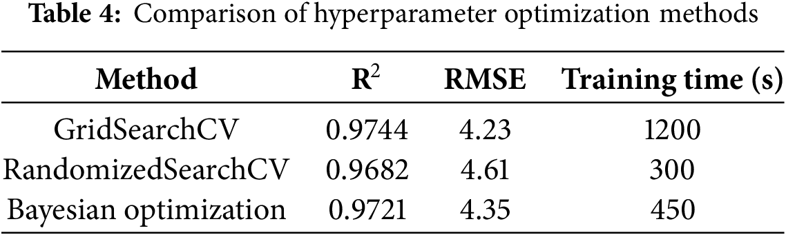
In this study, GridSearchCV, RandomizedSearchCV, and Bayesian Optimization are compared to demonstrate the advantages of GridSearchCV in fine hyperparameter tuning. Although GridSearchCV has a high computational overhead, it achieves the highest R2 and lowest RMSE by exhaustively enumerating all hyperparameter combinations to ensure that the global optimal solution is found, demonstrating its superior performance in terms of accuracy. In contrast, RandomizedSearchCV has an advantage in computational efficiency, but its accuracy is slightly lower than that of GridSearchCV. Although Bayesian Optimization can find a better solution with fewer searches, it may miss some of the best solutions because its optimization process is based on previous search results, so its accuracy is slightly inferior to GridSearchCV. This shows that GridSearchCV is the most suitable hyperparameter optimization method for fine parameter tuning in this study. The Table 4 shows the performance comparison of these three methods in XGBoost hyperparameter tuning:
Based on the aforementioned process, this paper proposes a PV power prediction model based on improved CNN-LSTM and cascading learning. The overall workflow is illustrated in Fig. 7, and the specific implementation steps are as follows:
(1) Data Collection and Preprocessing: Collect historical PV power data and meteorological data; handle missing values and outliers; perform feature selection (based on Pearson Correlation Coefficient (PCC) and Mutual Information (MI)) and standardize the data; split the dataset into training and test sets.
(2) 1D-CNN-LSTM Feature Extraction: Extract local features using 1D-CNN by learning the relationships among environmental variables over short periods through convolutional kernels; employ a two-layer LSTM to further model and extract long-term temporal dependencies.
(3) Cascading Learning: Use multiple base learners to combine the predictions with the original features layer by layer; determine whether to add additional cascading layers based on the average R2 value of each layer’s base learners to enhance the model’s expressive capacity; optimize the base learners using GridSearchCV.
(4) Fusion Layer Integration: Use XGBoost as the meta-learner to integrate and optimize the outputs of the cascading layers; further enhance model accuracy by optimizing the meta-learner using GridSearchCV.
(5) Model Evaluation and Iteration: Validate the model on the test set and evaluate its performance; if the model meets accuracy requirements, finalize the prediction model; otherwise, adjust parameters and iterate for further optimization.
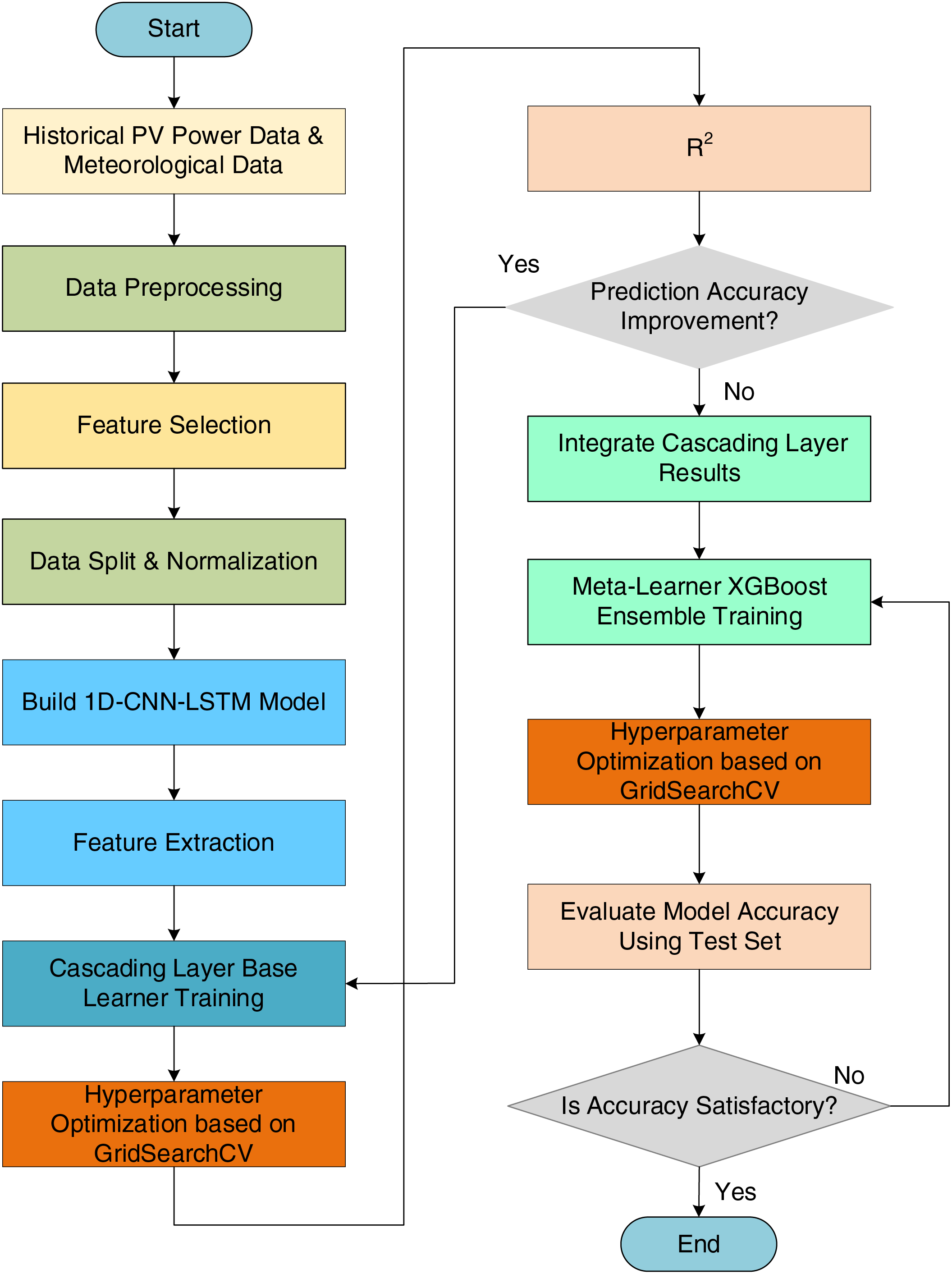
Figure 7: Photovoltaic power prediction process: improved CNN-LSTM and cascading learning methods
5 Calculated Case Validation Analysis
To verify the effectiveness of the proposed method, the experimental data were obtained from one year of monitoring data from a PV power station in Shanghai. Since the PV output of the power station is concentrated between 5:00 and 19:00, a 24-h ahead forecast is conducted for the 5:00–19:00 time period of the target day. The collected data are divided into a training set and a test set in an 8:2 ratio. The training set is used for training and establishing the prediction model, while the test set is used to evaluate the prediction performance of the model. Considering the impact of different weather conditions on PV power generation, the distribution of various weather types was analyzed: 100 sunny days, 102 partly cloudy days, 93 overcast days, and 71 rainy days. The PV power output is predicted for all four weather types.
5.1 Model Evaluation Metrics and Model Parameters
In this study, RMSE, MAE and R2 are used as evaluation metrics for the PV power prediction model. The expressions for RMSE and MAE are as follows:
where
5.2 Analysis of Base Learner Performance
To verify the suitability of base learners for the PV power prediction task, a detailed performance evaluation of various machine learning models was conducted under four different weather conditions. Fig. 8 presents the mean values of evaluation metrics for each model under the four weather conditions, while Table 5 shows the regression performance of each base learner under different weather scenarios. Based on the table and the corresponding bar charts, it can be seen that XGBoost and LightGBM exhibit high prediction accuracy across all weather conditions. Specifically, under sunny and partly cloudy conditions, LightGBM achieved R2 values of 0.970 and 0.957, respectively, while XGBoost reached R2 values of 0.975 and 0.960, demonstrating excellent fitting ability. Under more complex conditions such as overcast and rainy weather, XGBoost also achieved R2 values of 0.955 and 0.948, outperforming Random Forest (RF) and Support Vector Machine (SVM), and demonstrating superior robustness.
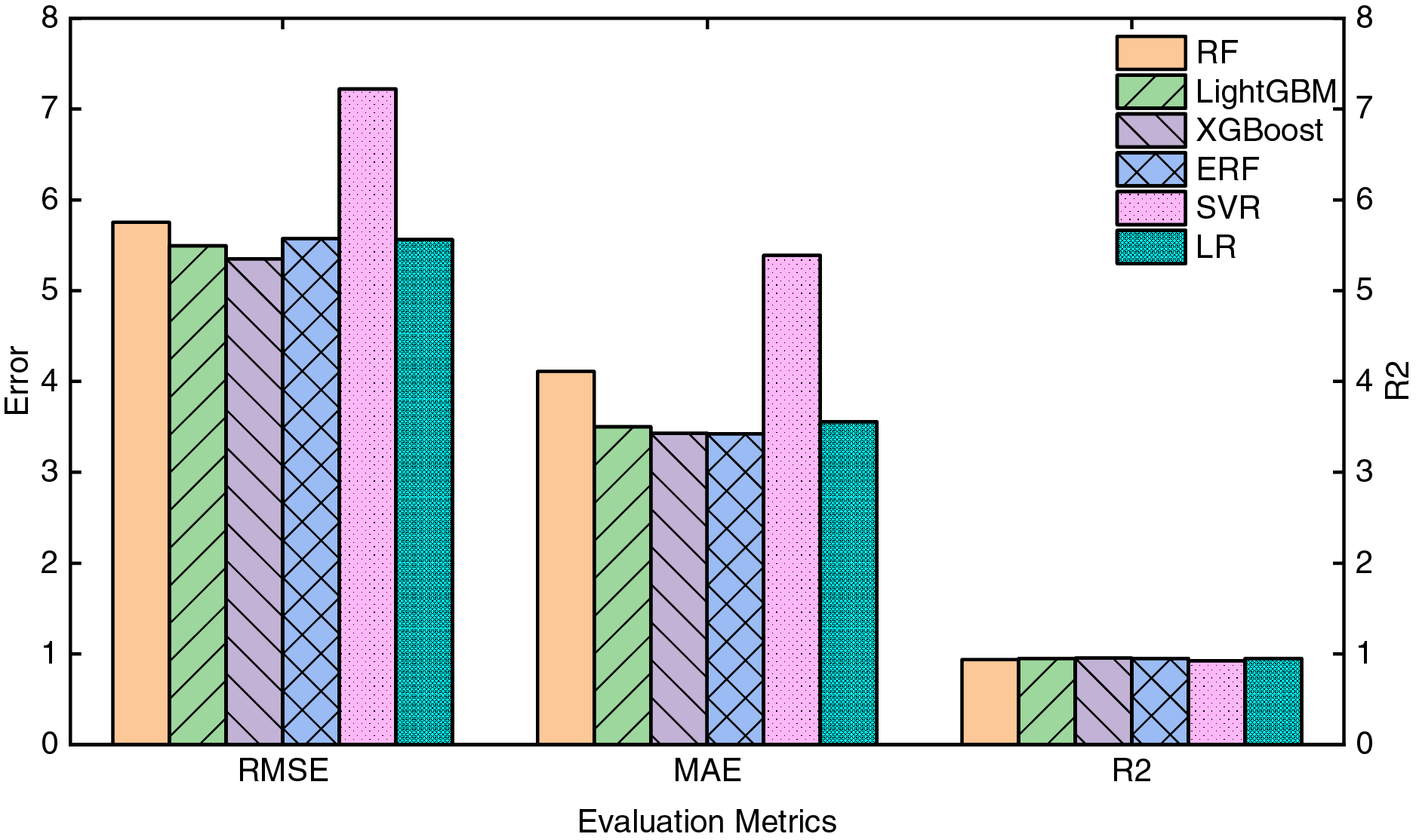
Figure 8: Comparison of average evaluation metrics for different models
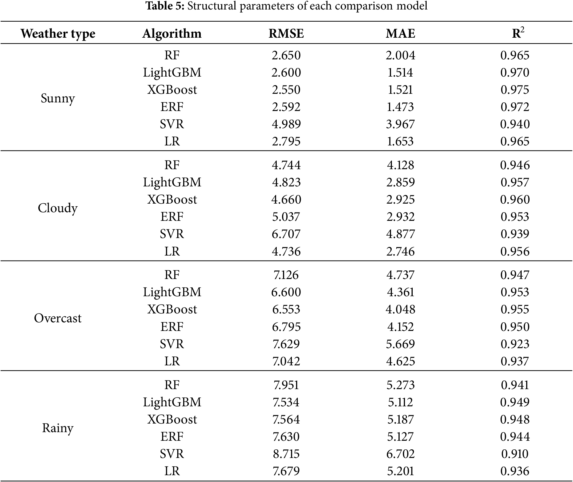
Especially under overcast and rainy conditions, where prediction becomes more challenging due to increased data variability, traditional Support Vector Machine models showed significantly higher RMSE values, with RMSE reaching 8.715 under rainy conditions, indicating insufficient capability to handle complex environmental fluctuations. Under the same conditions, XGBoost had an RMSE of 7.564 and an R2 of 0.948, indicating its stronger fitting capability when dealing with the nonlinear characteristics of PV power.
From the above analysis, it is evident that choosing XGBoost as the meta-learner in the cascading learning structure offers significant advantages. Firstly, XGBoost is capable of optimizing the model by minimizing prediction errors layer by layer and employing gradient boosting, which is particularly effective in handling complex nonlinear features. For example, under overcast conditions, XGBoost had an RMSE of 6.553, which was lower than that of RF (7.126), indicating its superior ability to capture features and reduce errors in complex environments. Additionally, as the meta-learner in the cascading structure, XGBoost effectively integrates the feature outputs of various base learners, leveraging the strengths of each model, which significantly enhances the generalization ability and prediction accuracy of the overall model, especially in response to varying weather conditions. The bar charts also visually illustrate the superior performance of XGBoost and LightGBM, which consistently demonstrate higher prediction accuracy and lower error compared to other traditional models across different weather conditions.
To validate the effectiveness of the adaptive cascading layer expansion strategy, this paper conducted a detailed analysis of the relationship between the number of cascading layers and model performance. The results are shown in Fig. 9. As the number of cascading layers increased, the model’s prediction performance, measured by R2, gradually improved. In this study, the threshold T is used to control the triggering condition of the cascade expansion in the model. When the R2 value of the model exceeds the threshold T, the cascade layer will be further expanded to improve the prediction accuracy. Specifically, the value of T is set to 0.95, which is adjusted in the experiment to ensure the best model performance. During the first and second cascading layers, the R2 value of the model rapidly increased from 0.956 to 0.967, indicating that adding cascading layers in the early stages significantly enhances the model’s predictive capability. Subsequently, the gains from the third to the fifth cascading layers diminished gradually and eventually stabilized, indicating that the model’s ability to represent data features had approached saturation as the number of layers increased. Specifically, after the fourth and fifth layers, the increment in R2 became minimal, confirming the effectiveness of the adaptive cascading layer expansion strategy. This strategy enables a reasonable control of the number of cascading layers while ensuring model accuracy, thereby avoiding unnecessary computational costs and potential overfitting issues. This performance-driven dynamic expansion mechanism ensures both the efficiency and the generalization capability of the model.
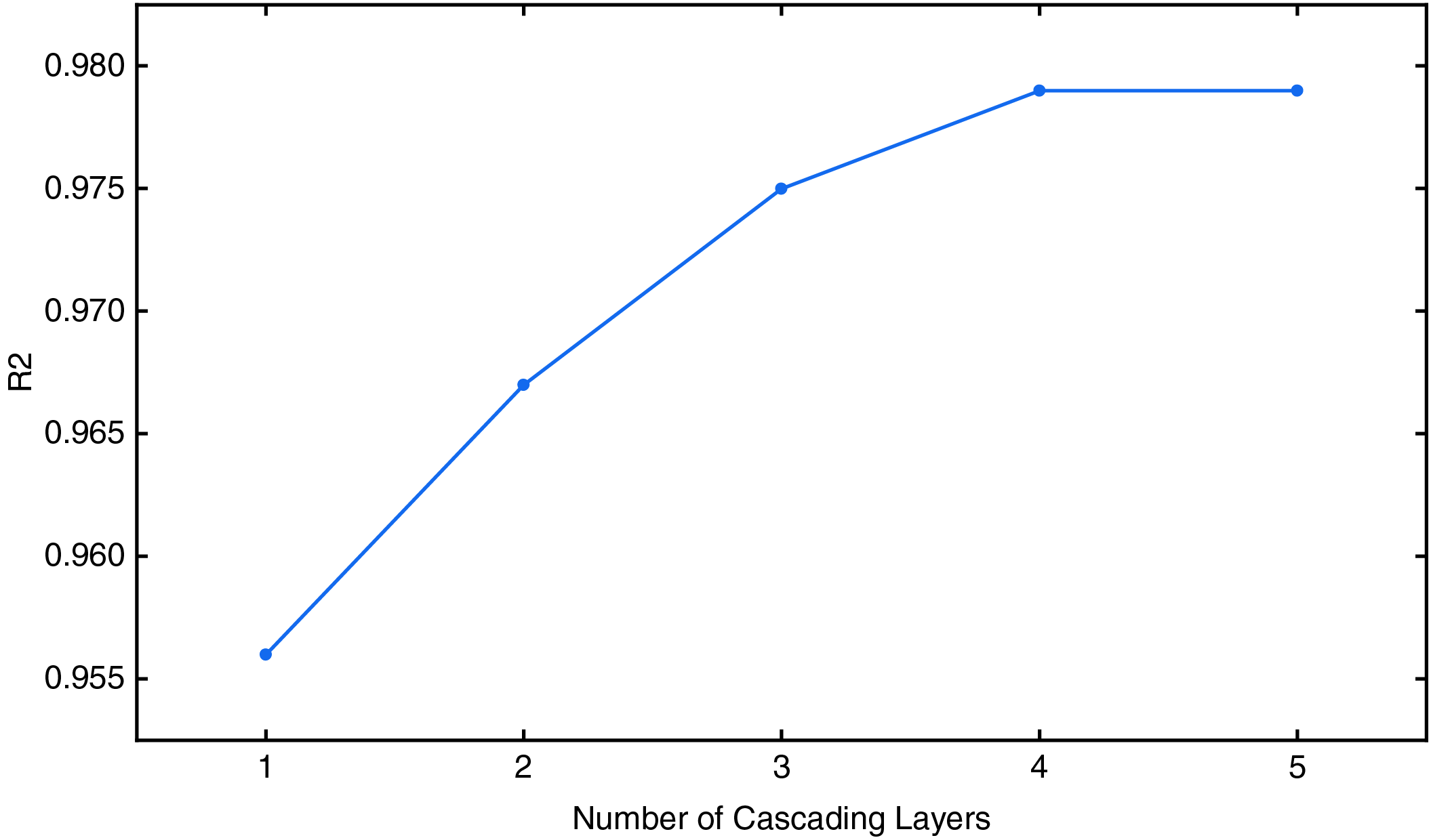
Figure 9: Relationship diagram between the number of cascade layer and R2
5.3 Comparison of Prediction Performance between the Proposed Model and Traditional Algorithms
To evaluate the proposed model against traditional prediction models under different weather conditions, comparative experiments were conducted, and the results are presented in Table 6. Combined with Figs. 10–13, it can be observed that the prediction curves of the proposed model exhibit the highest fit to the actual curves, accurately capturing the fluctuation trends of PV power. This demonstrates the accuracy and superiority of the proposed model in PV power prediction. The specific analysis is as follows:
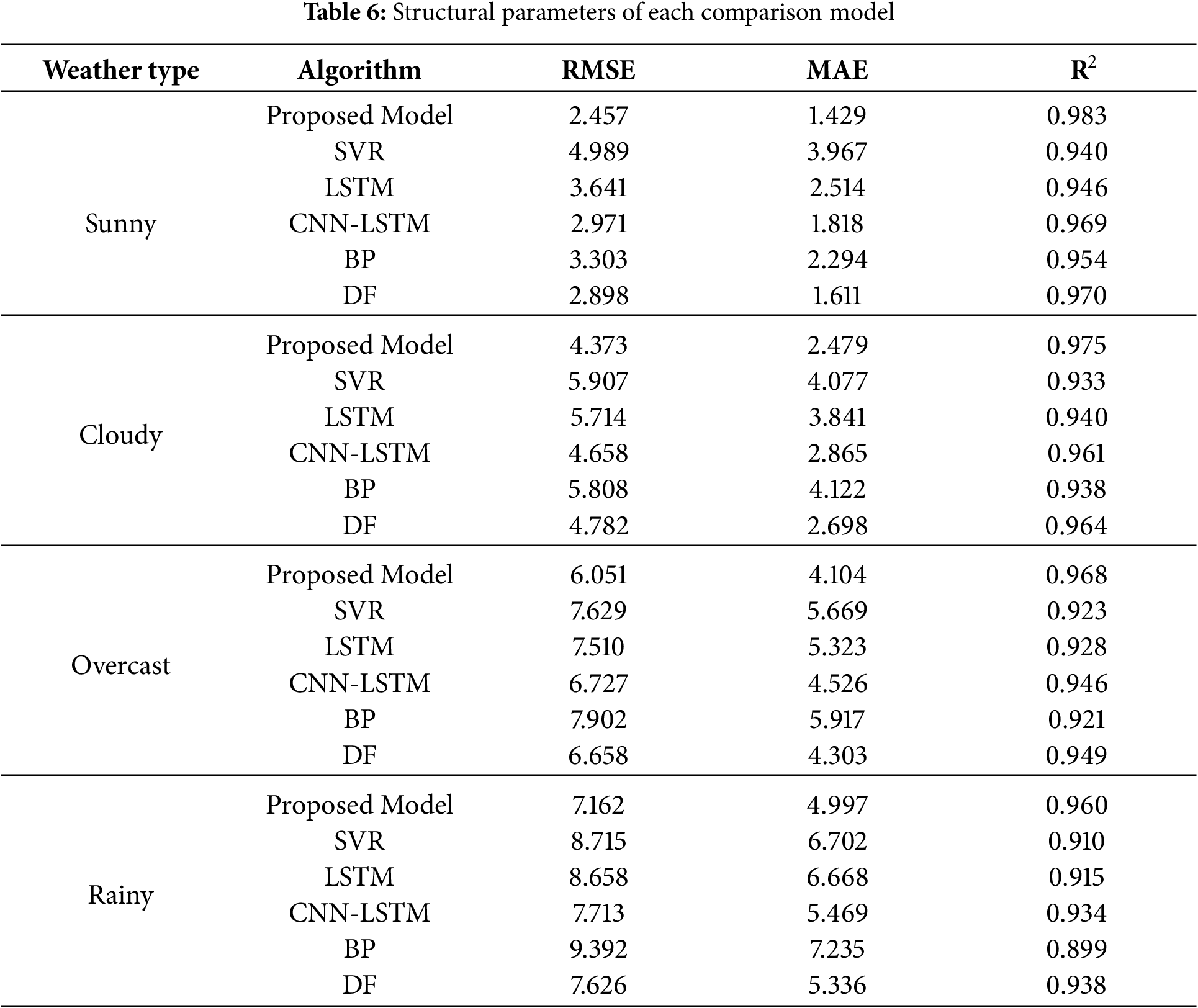

Figure 10: Prediction curves of each model under sunny weather
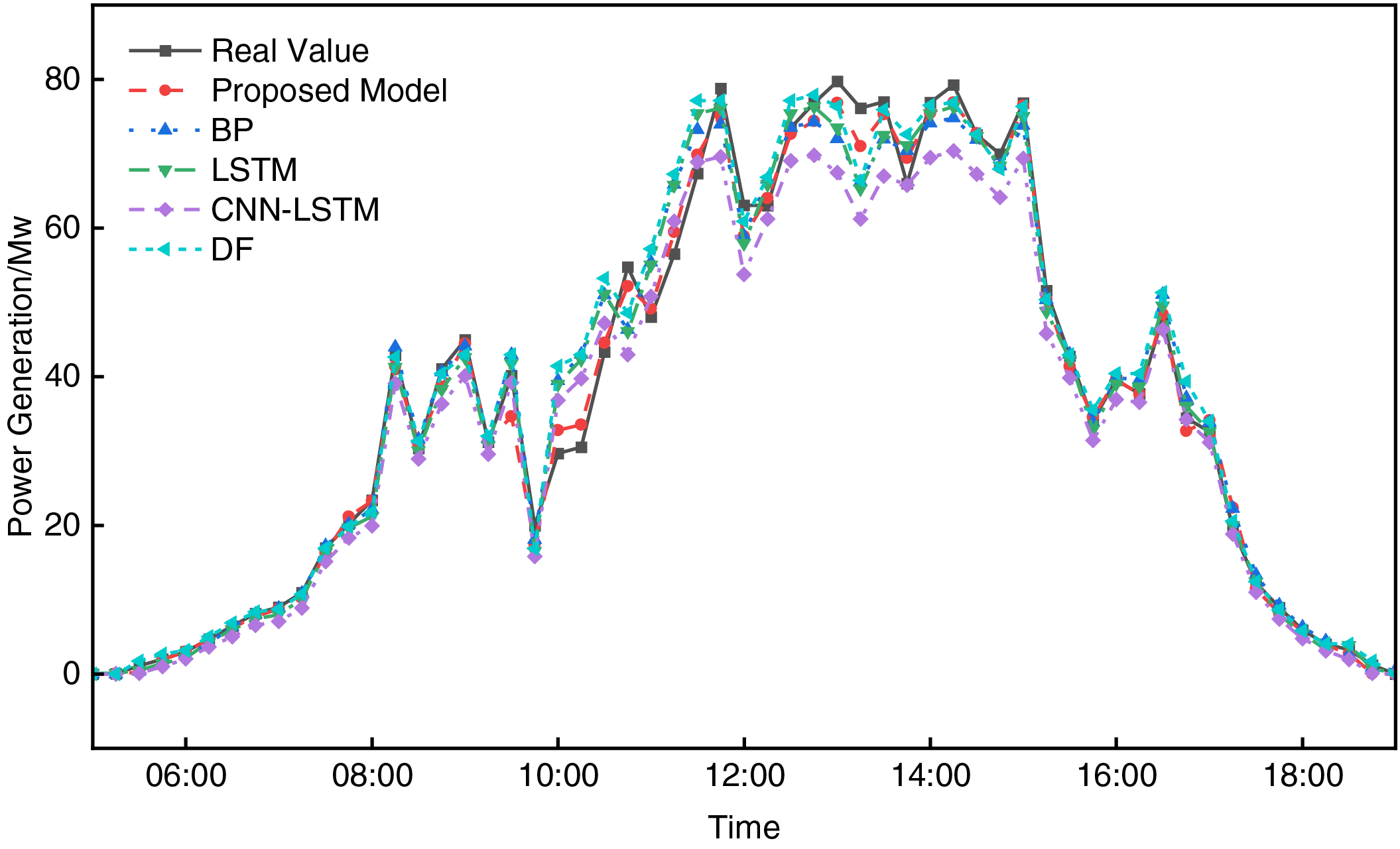
Figure 11: Prediction curves of each model under cloudy weather
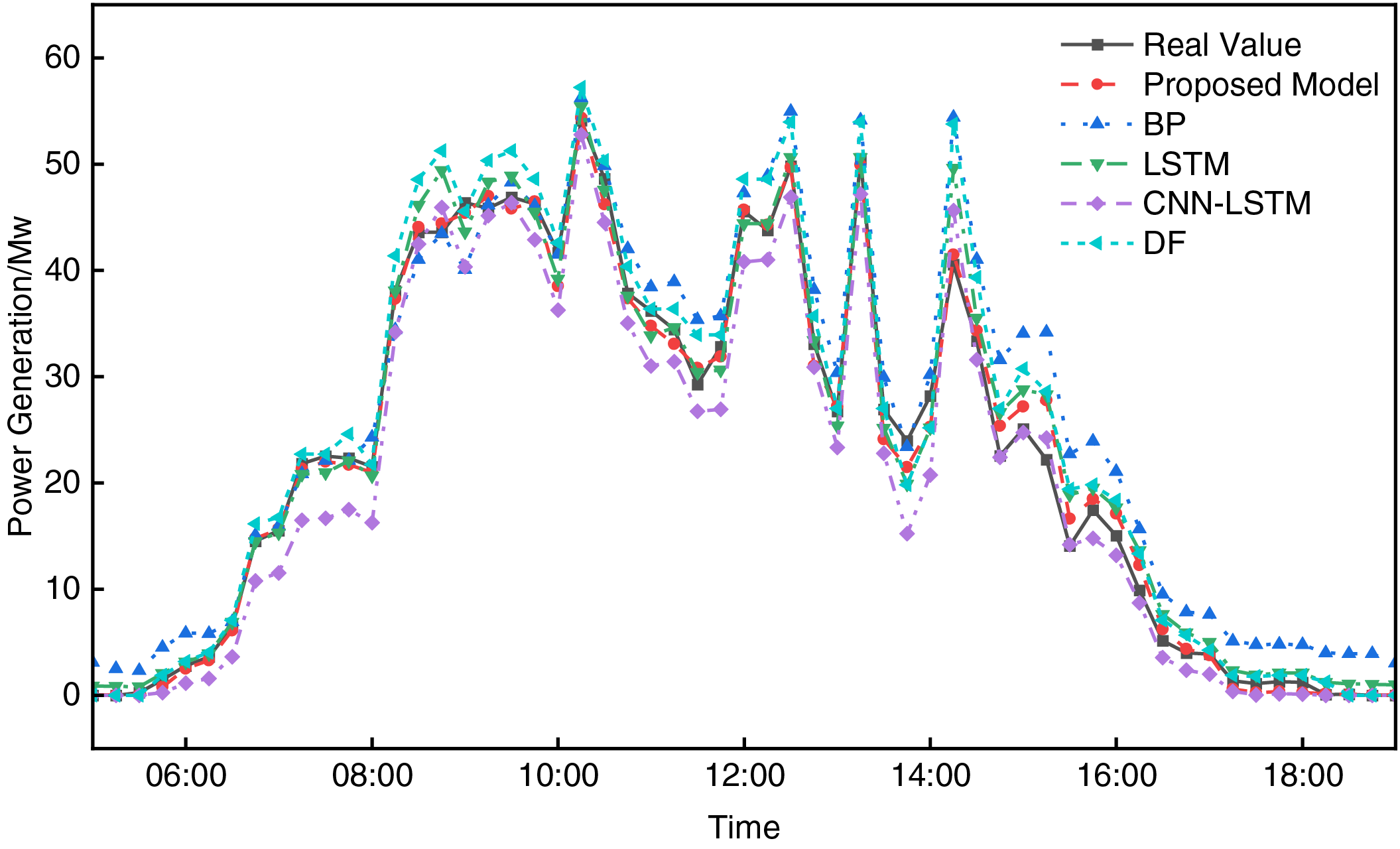
Figure 12: Prediction curves of each model under overcast weather
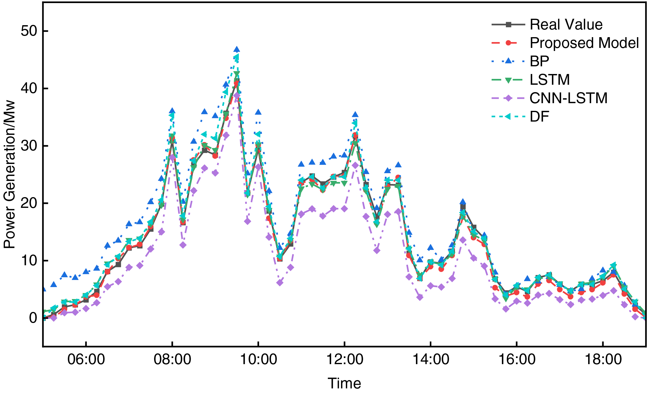
Figure 13: Prediction curves of each model under rainy weather
From Fig. 10 which shows the prediction curves under sunny conditions, and the data in Table 7, it can be seen that the proposed model exhibits significant predictive advantages under sunny conditions. The RMSE of the proposed model is 2.457, the MAE is 1.429, and the R2 reaches 0.983, all of which are superior to those of the comparison models. Notably, the proposed model accurately fits the dynamic changes of PV power during peak stages, whereas other models, such as SVR and LSTM, show significantly higher prediction errors, indicating their limitations in dealing with nonlinear and complex temporal features. In contrast, by combining 1D-CNN and LSTM for feature extraction and integrating with the cascading learning strategy, the proposed model successfully captures the temporal dependencies of PV power and demonstrates better prediction accuracy and robustness.
Fig. 11 shows the prediction curves under partly cloudy conditions. Under partly cloudy weather, the proposed model provides more accurate predictions, with all three metrics significantly outperforming the other models. Specifically, in conditions where the PV generation characteristics are complex and highly irregular due to the cloudy weather, the RMSE of SVR and LSTM were higher than that of the proposed model by 1.534 and 1.341, respectively, indicating that these models have limitations in dealing with the complex combination of nonlinear features. In contrast, the proposed improved model accurately predicts PV power under partly cloudy conditions, effectively capturing the fluctuation characteristics of PV power generation.
Fig. 12 shows the prediction curves under overcast conditions. Under overcast conditions, the uncertainty of the environment increases, and the influence of various meteorological factors on PV generation becomes more pronounced. The proposed model achieves an R2 of 0.968, which is superior to CNN-LSTM (0.946) and DF (0.949) comparison models. Furthermore, the RMSE of the proposed model is 6.051, which is significantly lower than those of SVR (7.629) and LSTM (7.510). This demonstrates that the proposed model can still effectively fit power output even in complex overcast environments, reflecting its ability to capture both temporal and nonlinear features comprehensively. In comparison, other models, especially traditional models, show insufficient fitting ability and struggle to accurately predict the fluctuations in PV power under overcast conditions.
Fig. 13 shows the prediction curves under rainy conditions. Under rainy conditions, PV power is most significantly affected by external factors, and power generation fluctuates drastically, which makes prediction particularly challenging. Even under such extreme conditions, the proposed model maintains high prediction accuracy, outperforming traditional models such as BP and DF. Notably, in the curve comparison under rainy conditions, the prediction curve of the proposed model fits the actual curve most closely, demonstrating strong generalization capability. In contrast, BP and SVR models had RMSE values of 9.392 and 8.715, respectively, failing to capture the dramatic changes in power generation, which resulted in higher errors. This further validates the effectiveness of the proposed dual ensemble strategy in handling PV power prediction under complex meteorological conditions.
The model in this paper is used to perform performance tests on the second dataset of the National Energy Rixin Photovoltaic Power Forecasting Competition. The data sampling frequency is 15 min/time, which includes environmental factors such as irradiance, pressure, temperature and humidity, wind speed and direction, which are basically consistent with the meteorological factors in the dataset of this paper. Fig. 14 shows the prediction results of the proposed model for the new dataset. As can be seen from the figure, the model can capture the overall trend of the data, especially in the rising and falling stages, but the predicted value and the actual value are slightly deviated in extreme cases. The experimental results show that the proposed model has high accuracy on the new dataset, with an R2 value of 0.96, RMSE and MAE of 4.45 and 2.81, respectively, and the error has decreased, further proving the effectiveness and robustness of the model. To further optimize the accuracy of the model, we plan to explore methods such as data enhancement, transfer learning, and multi-task learning in future work.
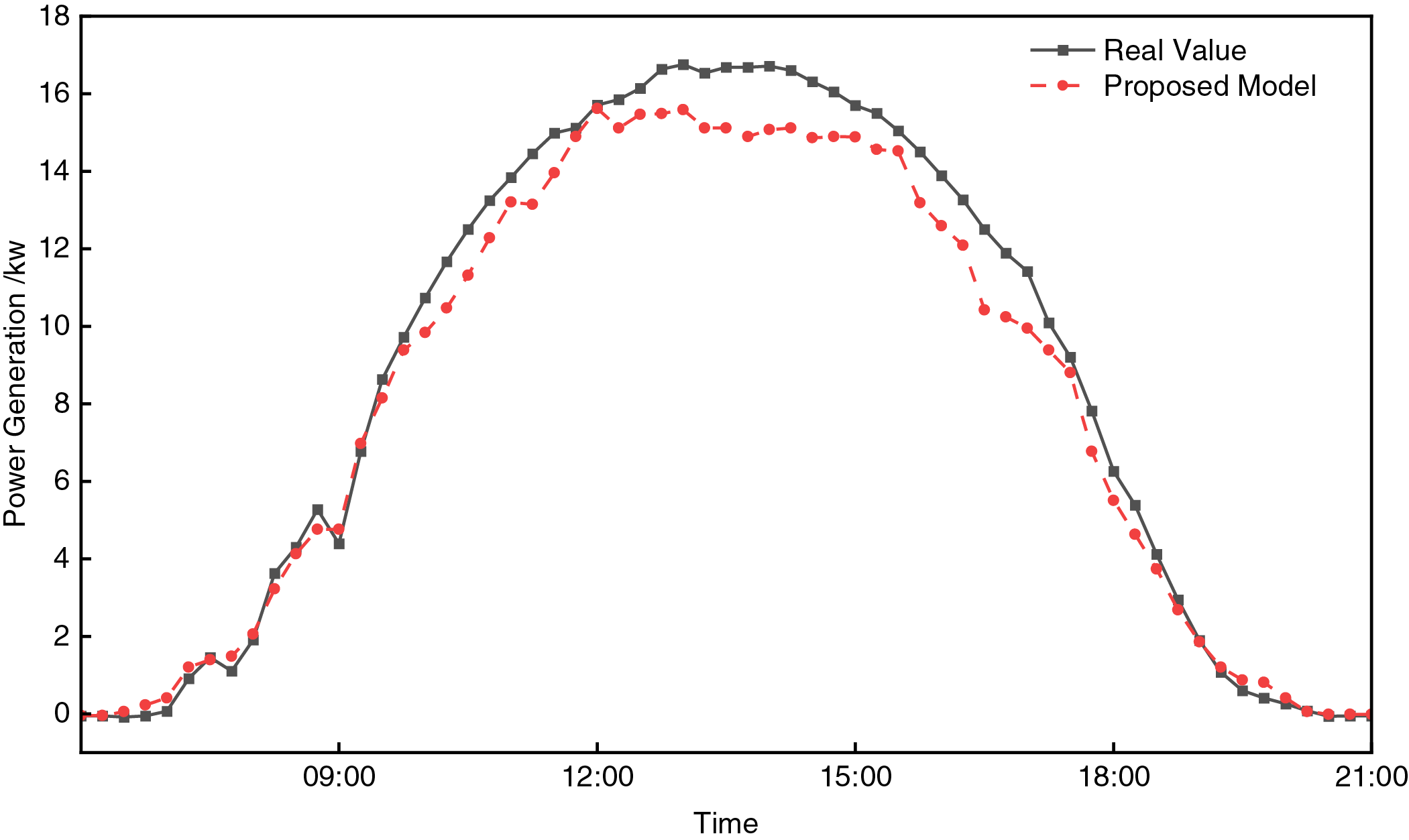
Figure 14: Prediction curve of this model in the public dataset
5.4 Ablation Experiment Design
To validate the effectiveness of each module in the proposed model, an ablation experiment was conducted by progressively removing key modules from the model and evaluating their impact on the performance of PV power prediction. The evaluation metrics for the ablation experiment are presented in Table 5. The ablation experiment is based on mixed weather data (sunny, cloudy, overcast and rainy days each account for 1/4), which cannot be directly compared with the single weather results in Table 4. As can be seen from the table, the proposed model achieves optimal performance across all metrics, demonstrating the significant effect of the synergy between the modules in improving prediction accuracy. After removing the 1D-CNN-LSTM module, the RMSE increased by 0.741 and the R2 decreased by 1%, indicating that the 1D-CNN-LSTM feature extraction module is crucial for capturing both local features and temporal dependencies.
When some base learners were removed from the cascading structure, the RMSE increased to 5.097 and the R2 decreased by 2.1%, suggesting that the collaboration among multiple base learners is essential for capturing diverse feature information. Furthermore, after removing the meta-learner and the dynamic cascading layer expansion strategy, the model’s performance was significantly affected, with RMSE increasing by 1.394 and 1.708, respectively, compared to the proposed model, and R2 decreasing by 1.9% and 2.2%, respectively. This indicates that the meta-learner integration strategy effectively combines the features from all cascading layers to enhance the overall prediction capability, while the dynamic cascading layer expansion strategy ensures a balance between model complexity and generalization capability.
After removing hyperparameter optimization, the RMSE increased to 5.356 and the R2 dropped to 0.958, which suggests that the optimized parameters significantly contribute to model performance.
The results of the ablation experiment demonstrate that each module in the proposed model plays a significant role in enhancing the performance of PV power prediction. The collaborative optimization of all modules endows the final model with high prediction accuracy and robustness under complex environmental conditions.
This paper proposes a PV power prediction model based on an improved CNN-LSTM and cascading learning strategy to address the challenges of complex environmental variables and difficulties in temporal feature modeling for PV power prediction. Based on the specific case study, the following conclusions are drawn:
(1) The use of the CNN-LSTM network for deep feature extraction effectively captures both local features and temporal dependencies, significantly improving the prediction accuracy of the model and its adaptability to dynamic environmental changes. Experimental results indicate that the proposed model maintains high prediction accuracy and robustness under different weather conditions, effectively achieving the research objectives.
(2) By constructing a multi-layer cascading learning structure, base learners such as LightGBM, XGBoost, Random Forest, and Extreme Random Forest are introduced layer by layer for feature fusion. XGBoost is used as the meta-learner to integrate the outputs of the base learners and produce the final prediction result, greatly enhancing the model’s ability to represent complex features. The cascading structure progressively optimizes the prediction performance, and the integration strategy using XGBoost as the meta-learner effectively combines the strengths of multiple base learners, significantly enhancing the overall generalization ability and prediction accuracy of the model.
(3) This paper proposes a dynamic cascading layer expansion strategy based on R2 performance, where each layer is evaluated to determine whether to expand the cascading structure, thereby enhancing the prediction capability of the model while avoiding unnecessary computation and overfitting. The dynamic expansion strategy is based on the R2 threshold (T = 0.95), and its adaptability needs to be further verified. In the future, data from multiple regions (such as Xinjiang and Guangdong) will be collected to test the generalization of the model. The current results show that the R2-driven dynamic strategy can adaptively adjust the cascade depth, reduce the risk of overfitting, and is suitable for different climate modes. Experimental results show that this dynamic expansion strategy increases the model’s flexibility, allowing it to maintain high performance even under complex environmental conditions. The proposed improved model provides an effective solution for intelligent PV power prediction and can be extended to other types of time series data prediction, with promising applications and practical value.
Acknowledgement: Not applicable.
Funding Statement: 2023 Sustainable Development Science and Technology Innovation Action Plan Project of Chongming District Science and Technology Committee, Shanghai (CKST2023-01). Shanghai Science and Technology Commission Funded Project (19DZ2254800).
Author Contributions: Conceptualization, Methodology, Supervision, Chen Yang; Data curation, Writing—original draft, Feng Guo; Design, Data interpretation, Dezhong Xia; Writing—review & editing, Validation, Visualization, Investigation, Jingxiang Xu. All authors reviewed the results and approved the final version of the manuscript.
Availability of Data and Materials: Not applicable.
Ethics Approval: Not applicable.
Conflicts of Interest: The authors declare no conflicts of interest to report regarding the present study.
Nomenclature
| PV | Photovoltaic |
| CNN | Convolutional Neural Network |
| LSTM | Long Short-Term Memory |
| CNN-LSTM | Convolutional Neural Network-Long Short-Term Memory |
| RF | Random Forest |
| ERF | Extreme Random Forest |
| XGBoost | Extreme Gradient Boosting |
| LightGBM | Light Gradient Boosting Machine |
| ARIMA | Autoregressive Integrated Moving Average |
| IQR | Inter Quartile Range |
| GHI | Global Horizontal Irradiance |
| DNI | Direct Normal Irradiance |
| DHI | Diffuse Horizontal Irradiance |
| AT | Actual Temperature |
| MT | Module Temperature |
| AH | Actual Humidity |
| AAP | Actual Atmospheric Pressure |
| AWS | Actual Wind Speed |
| AWD | Actual Wind Direction |
| MI | Mutual Information |
| PCC | Pearson Correlation Coefficient |
| 1D-CNN | 1D Convolutional Neural Network |
| RNN | Recurrent Neural Network |
| GBDT | Gradient Boosting Decision Tree |
| GridSearchCV | Grid Search with Cross Validation |
| DF | Deep Forest |
| R2 | Coefficient of Determination |
| RMSE | Root Mean Square Error |
| MAE | Mean Absolute Error |
| BP | Back Propagation |
| SVR | Support Vector Regression |
| LR | Linear Regression |
References
1. Xin B, Shan B, Li Q, Yan H, Wang C. Rethinking of the three elements of energy toward carbon peak and carbon neutrality. Proc CSEE. 2022;42(9):3117–26. doi:10.13334/j.0258-8013 (In Chinese). [Google Scholar] [CrossRef]
2. Peng SJ, Lu J, Zhang ZD. Research on the influence of photovoltaic access on a power grid. Power Syst Prot Control. 2021;49(5):157–64. doi:10.19783/j.cnki.pspc.200505 (In Chinese). [Google Scholar] [CrossRef]
3. Qiu TZ, Wang LC, Lu YB. Potential assessment of photovoltaic power generation in China. Renew Sustain Energy Rev. 2022;154:111900. [Google Scholar]
4. Zhang ZF, da Silva FF, Guo YF. Coordinated voltage control in unbalanced distribution networks with two-stage distributionally robust chance-constrained receding horizon control. Renew Energy. 2022;198:907–15. [Google Scholar]
5. Zhu QF, Li JT, Qiao J. Application and prospect of artificial intelligence technology in renewable energy forecasting. Proc CSEE. 2023;43(8):3027–48. doi:10.13334/j.0258-8013.pcsee.213114 (In Chinese). [Google Scholar] [CrossRef]
6. Chen XH, Song YX, Zhang LG, Yuan W. Ultra-short-term power prediction of distributed photovoltaic driven by model and data hybrid. Distrib Util. 2023;40(1):2–9. doi:10.19421/j.cnki.1006-6357.2023.01.001 (In Chinese). [Google Scholar] [CrossRef]
7. FZhou CE, Sun PG. A novel weather classification method and its application in photovoltaic power prediction. J Shanghai Jiaotong Univ. 2021;55(2):1510–9. doi:10.16183/j.cnki.jsjtu.2021.264 (In Chinese). [Google Scholar] [CrossRef]
8. Pu ZY, Xia P, Zhang L. Comparative analysis of machine learning and statistical approaches for solar energy forecasting. Acta Energiae Solaris Sin. 2023;44(7):162–7. doi:10.19912/j.0254-0096.tynxb.2022-90 (In Chinese). [Google Scholar] [CrossRef]
9. Mayer JM, Gróf G. Extensive comparison of physical models for photovoltaic power forecasting. Appl Energy. 2021;283:116239. [Google Scholar]
10. Zhao BB, Wang Y, Wang B. Photovoltaic power prediction in distribution network based on ARIMA model time series. Renew Energy Resour. 2019;37(6):820–3. doi:10.13941/j.cnki.21-1469/tk.2019.06.005 (In Chinese). [Google Scholar] [CrossRef]
11. Yu M, Niu D, Wang K, Du R, Yu X, Sun L, Wang F. Short term photovoltaic output interval prediction based on integrated machine learning model. Smart Power. 2024;52(2):87–93, 107. doi:10.1016/j.energy.2023.127348 (In Chinese). [Google Scholar] [CrossRef]
12. Wan A, Chang Q, Khalil AB, He J. Short-term power load forecasting for combined heat and power using CNN-LSTM enhanced by attention mechanism. Energy. 2023;282:128274. doi:10.1016/j.energy.2023.128274. [Google Scholar] [CrossRef]
13. Zhang Y, Pan Z, Wang H, Wang J, Zhao Z, Wang F. Achieving wind power and photovoltaic power prediction: an intelligent prediction system based on a deep learning approach. Energy. 2023;283:129005. doi:10.1016/j.energy.2023.129005. [Google Scholar] [CrossRef]
14. Hochreiter S. Long short-term memory. Neural Comput. 1997;9(8):1735–80. doi:10.1162/neco.1997.9.8.1735. [Google Scholar] [PubMed] [CrossRef]
15. Wang D, Gan J, Mao J, Chen F, Yu L. Forecasting power demand in China with a CNN-LSTM model including multimodal information. Energy. 2023;263(1):126012. doi:10.1016/j.energy.2022.126012. [Google Scholar] [CrossRef]
16. Chen YF, Ma XY, Cheng K. Ultra-Short-Term power forecasting of renewable energy based on meteorological feature selection and SVM model parameter optimization. Acta Energiae Solaris Sin. 2023;44(12):568–76. doi:10.19912/j.0254-0096.tynxb.2022-1401 (In Chinese). [Google Scholar] [CrossRef]
17. Liu JC, Liu J, Zhao HY. Short-term photovoltaic output forecasting based on diffusion kernel density estimation and improved max-relevance and min-redundancy feature selection. Autom Electr Power Syst. 2021;45(14):13–21, (In Chinese). [Google Scholar]
18. Abou HM, Bukhari SMS, Zafar MH, Mansoor M, Chen W. COA-CNN-LSTM: coati optimization algorithm-based hybrid deep learning model for PV/wind power forecasting in smart grid applications. Appl Energy. 2023;349(3):121638. doi:10.1016/j.apenergy.2023.121638. [Google Scholar] [CrossRef]
19. Marinho FP, Rocha PA, Neto AR, Bezerra FD. Short-term solar irradiance forecasting using CNN-1D, LSTM, and CNN-LSTM deep neural networks: a case study with the Folsom (USA) dataset. J Sol Energy Eng. 2023;145(4):041002. doi:10.1115/1.4056122. [Google Scholar] [CrossRef]
20. Wu XZ, Wang ZY, Dai W. Bi-ensembled Photovoltaic (PV) power prediction based on heterogeneous clustering and stacking. Power Syst Technol. 2023;47(1):275–84. doi:10.13335/j.1000-3673.pst.2022.0408 (In Chinese). [Google Scholar] [CrossRef]
21. Chen T, Guestrin C. XGBoost: a scalable tree boosting system. In: Proceedings of the 22nd ACM SIGKDD International Conference on Knowledge Discovery and Data Mining; 2016 Aug 13–17; San Francisco, CA, USA. p. 785–94. [Google Scholar]
22. Ke G, Meng Q, Finley T, Wang T, Chen W, Ma W, et al. LightGBM: a highly efficient gradient boosting decision tree. In: 31st Conference on Neural Information Processing Systems (NIPS 2017); 2017 Dec 4–9; Long Beach, CA, USA. [Google Scholar]
23. Rigatti SJ. Random forest. J Insur Med. 2017;47(1):31–9. doi:10.17849/insm-47-01-31-39.1. [Google Scholar] [PubMed] [CrossRef]
24. Rasheed S, Kumar GK, Rani DM, Kantipudi MVP, Anila M. Heart disease prediction using gridsearchcv and random forest. EAI Endorsed Trans Pervasive Health Technol. 2024;10(1):1. [Google Scholar]
25. Zhou ZH, Feng J. Deep forest. Natl Sci Rev. 2018;6(1):74–86. [Google Scholar] [PubMed]
Cite This Article
 Copyright © 2025 The Author(s). Published by Tech Science Press.
This work is licensed under a Creative Commons Attribution 4.0 International License , which permits unrestricted use, distribution, and reproduction in any medium, provided the original work is properly cited.
 Downloads
 Citation Tools