
 Submit a Paper
 Propose a Special lssue
 Open Access
ARTICLE

Ultrashort-Term Power Prediction of Distributed Photovoltaic Based on Variational Mode Decomposition and Channel Attention Mechanism
1 Intelligent Distribution Network Department, Inner Mongolia Electric Power Economics and Technology Research Institute, Hohhot, 010020, China
2 Key Laboratory of Modern Power System Simulation and Control & Renewable Energy Technology, Ministry of Education (Northeast Electric Power University), Jilin, 132012, China
3 Production Technology Department, Inner Mongolia Power (Group) Co. Ltd., Hohhot, 010010, China
* Corresponding Author: Junhui Li. Email:
Energy Engineering 2025, 122(6), 2155-2175. https://doi.org/10.32604/ee.2025.062218
Received 12 December 2024; Accepted 10 March 2025; Issue published 29 May 2025
 View Full Text
 Download PDF
Abstract
Responding to the stochasticity and uncertainty in the power height of distributed photovoltaic power generation. This paper presents a distributed photovoltaic ultra-short-term power forecasting method based on Variational Mode Decomposition (VMD) and Channel Attention Mechanism. First, Pearson’s correlation coefficient was utilized to filter out the meteorological factors that had a high impact on historical power. Second, the distributed PV power data were decomposed into a relatively smooth power series with different fluctuation patterns using variational modal decomposition (VMD). Finally, the reconstructed distributed PV power as well as other features are input into the combined CNN-SENet-BiLSTM model. In this model, the convolutional neural network (CNN) and channel attention mechanism dynamically adjust the weights while capturing the spatial features of the input data to improve the discriminative ability of key features. The extracted data is then fed into the bidirectional long short-term memory network (BiLSTM) to capture the time-series features, and the final output is the prediction result. The verification is conducted using a dataset from a distributed photovoltaic power station in the Northwest region of China. The results show that compared with other prediction methods, the method proposed in this paper has a higher prediction accuracy, which helps to improve the proportion of distributed PV access to the grid, and can guarantee the safe and stable operation of the power grid.Keywords
With China’s increasing demand for energy and the growing environmental problems, the vigorous development of clean and renewable energy has captured widespread attention [1]. Distributed photovoltaic (DPV) power generation, as a clean and sustainable energy source, has the advantage of low installation and maintenance costs [2]. DPV is important in improving China’s energy demand and environmental issues. As of September 2024, China’s installed DPV capacity has reached 341.91 million kilowatts [3]. However, DPV power is affected by various meteorological factors and geographic locations, resulting in significant volatility and uncertainty, which poses a considerable challenge and test to the supply-demand balance and safe operation of the power grid [4]. Therefore, high precision prediction of PV power is of great significance, which can not only reduce the uncertainty of PV grid connection and guarantee the stable operation of the power system, but also enhance the PV consumption capacity and PV power generation efficiency.
For the issue of DPV power forecasting, researchers both domestically and internationally have conducted extensive research, and the prediction methods include physically-driven prediction, data statistical methods, and artificial intelligence algorithms [5]. The physically driven prediction method is based on the characteristics of PV cells, installation angle, and other physical parameters, and combined with the PV cell output characteristic curve to construct a prediction model, using the data provided by the numerical weather prediction, accurate prediction of future PV power [6,7]. The accuracy of this method relies on parameter resolution during the modeling process. and the accuracy of the numerical weather forecast. Data statistical methods do not need specific physical parameters of PV power plants, through the in-depth analysis of historical data, using statistical models and algorithms to find the potential correlation and law between historical data, to predict the PV power generation power of the next period [8]. Data statistical prediction methods mainly include autoregression and moving average model [9], multiple regression methods [10], Markov chain model [11], and support vector machine model [12]. The above models mainly make predictions by mining the mapping laws between the inputs and outputs of the prediction model, and when the time series is highly nonlinear, both the accuracy and robustness of their predictions are affected.
In recent years, continuous breakthroughs in advanced technologies such as deep learning have opened up new paths for accurately predicting distributed PV output. Deep learning has excellent feature extraction and nonlinear fitting capabilities and is widely used for PV power prediction [13,14]. Tajjour et al. [15] migration learning is introduced to train deep neural networks using solar radiation data, significantly enhancing PV power prediction accuracy. Ren et al. [16] proposed a Quad-kernel deep CNN model to harness data correlations and enhance PV prediction accuracy effectively. Liu et al. [17] proposed a new weather classification method and important meteorological features were extracted and input into an improved LSTM model to accurately predict photovoltaic power generation. Dai et al. [18] used the random forest approach to extract important features, inputting features into the RepeatVector layer and the TimeDistributed layer into the Gated Recurrent Unit to enhance PV power prediction accuracy. Hao et al. [19] proposed an improved temporal convolutional network model and the introduction of a multi-scale time module that captures dependencies between complex data. However, the process of utilizing a single neural network for output prediction of distributed photovoltaics faces dual challenges in terms of prediction accuracy and training time. Incorporating the advantages of multiple deep learning models becomes an effective strategy to improve prediction accuracy. Agga et al. [20] proposed a hybrid deep learning model combining CNN and LSTM, where the CNN captures spatial features and the LSTM extracts temporal dependencies. Limouni et al. [21] combined LSTM and TCN, with LSTM, used to capture temporal features in the data, and the connection relationship between the extracted temporal features and the output is established through TCN to output the PV prediction results. Zhou et al. [22] predicted photovoltaic power by combining three different neural networks CNN-LSTM-attention to form a new hybrid model. Xu et al. [23] combined GRU and XGBoost models to predict PV power.
The above prediction mainly uses a CNN to extract spatial features, but no attention is paid to the weight component of the extracted spatial features. At the same time, LSTM only noticed the one-way data information and did not take into account the influence of the reverse data information. BiLSTM can synthesize the forward and reverse evolutionary patterns of data sequences. Rao et al. [24] combined three-layer BiLSTM and a deep neural network to fully mine the inter-data features input into a deep neural network to improve the accuracy of PV prediction.
The findings of this research indicate that integrating the features of various deep learning models can enhance the prediction accuracy of nonlinear and nonsmooth sequences. However, existing approaches have not yet developed models specifically designed to address the unique characteristics of DPV data. In addition to constructing hybrid neural network models, existing research has also applied various signal decomposition techniques in the field of distributed PV prediction, mainly aiming to improve prediction accuracy and reduce the non-stationarity and uncertainty in PV data. Kong et al. [25] reduced the noise of solar radiation data by empirical mode decomposition, inputting data into GRU and Attention Mechanism model, where Attention Mechanism focuses on important features, and finally obtained solar radiation data. EMD is prone to modal aliasing when processing nonlinear time series. VMD decomposes the original signal into a specified number of non-recursive variable modes, which can be a good alternative to EMD. Zhao et al. [26] aimed at the problem of poor accuracy of severe weather prediction, the prediction model of VMD-KELM is proposed, which uses VMD to decompose the historical data, inputs the data into the KELM model, and finally outputs the PV prediction results.
This paper presents a distributed photovoltaic ultra-short-term power forecasting method based on VMD and Channel Attention Mechanism. The main contributions of this paper are as follows:
(1) By combining VMD decomposition with the cosine correlation coefficient, non-stationary noise is eliminated and the computational time of the neural network is reduced through the decomposition and reconstruction of the data.
(2) A new hybrid prediction model is proposed, which includes CNN, channel attention mechanism, and BiLSTM. The channel attention mechanism can effectively extract high-dimensional space features and dynamically adjust weights.
(3) A robust preprocessing framework is provided for distributed photovoltaic data with small sample size and high noise.
Through the analysis of a distributed PV power plant dataset from Northwest China and a comparison with existing methods, the proposed approach demonstrates superior prediction accuracy and holds significant value for engineering applications.
The paper is organized as follows: The second part of this paper introduces the principle of distributed PV decomposition and reconstruction; the third part introduces the deep learning model construction of this paper incorporating the channel attention mechanism; the fourth part introduces the ultrashort-term power prediction process of DPV power generation based on the variational pattern decomposition and the channel attention mechanism; the fifth part includes the conditions of the arithmetic case, the data preprocessing, the feature extraction, and the model evaluation indexes as well as the part of the analysis of arithmetic case; and the sixth part is divided into the conclusion of this paper.
2 Distributed Photovoltaic Power Decomposition and Reconstruction
The output of distributed PV is influenced by various external uncertainties, especially the fluctuation of weather conditions, which leads to a complex non-stationarity in its time-series characteristics. To realize the ultra-short-term and high-precision prediction of distributed PV power generation, the intrinsic mechanism of the non-stationary characteristics needs to be revealed. VMD exhibits noise immunity and robust properties when dealing with non-stationary signals [26]. Therefore, this paper proposes to decompose the distributed PV historical data using variational modal decomposition, which aims to effectively decompose the non-stationary time-series features of distributed PV power generation into multiple narrow-band signal components with varying center frequencies, and never to reduce the complexity of distributed PV time series.
The specific steps of VMD decomposition are:
The input raw signal f(t) is first decomposed to obtain a set of modal functions uk(t) in which each mode uk(t) is a finite bandwidth signal with a specific center frequency
Each submodule uk(t) does not have the same center frequency
(1) Hilbert variation of each submodule uk(t) to obtain its one-sided spectral function.
(2) Convert the frequency of each sub-mode to its corresponding fundamental frequency band, and the predicted center frequency
(3) Based on the results of the L2 paradigm of the modulated signal described above, the bandwidth of each submodule is evaluated and the bandwidth range of each submodule is determined. The objective function is given as:
(4) The above constrained extreme value problem is converted into an unconstrained variational problem to be solved using the Lagrange multiplier operator
(5) The unconstrained variational problem that has been transformed is solved used the alternating direction approach multiplicative operators and the optimization model is updated as shown below.
where:
(6) During iterations, the algorithm is considered to have converged and the iterations are stopped by comparing the magnitude of the change in mode
where:
The above formula is the termination condition in the algorithm, which is used to determine whether the iteration can end or not.
The choice of the number of components k is of great significance when decomposing the original signal. If k is set to a small value, it may trigger the phenomenon of modal under-decomposition, which may reduce the accuracy of prediction; while too large a value of k may lead to overlapping of modes or the introduction of unwanted noise. To determine the optimal k value, different k are set and the center frequency of each component is calculated for each k value.
Since decomposing several different sub-modalities may lead to the problem of excessive computation, it reduces the subsequent computation. The different historical power curves are reconstructed by calculating the correlation between each modality after decomposition and historical power for combination. The cosine value of the sub-modal and historical PV power is utilized as an evaluation criterion, which is calculated by the formula:
where:
The closer the magnitude of the cosine value is to 1, the more relevant the modal component is to the generation power. Selecting components with high correlation for reconstruction to remove noisy data can simultaneously cut down the computational complexity of the model.
3 Deep Learning Model Construction for Fusing Channel Attention Mechanisms
3.1 Spatial Feature Extraction
Ultra-short-term power prediction for distributed PV faces significant nonlinear and stochastic challenges, while traditional statistical methods make it difficult to fully capture the complex features of the input data. CNN, as a feed-forward neural network architecture, significantly reduces the number of weight parameters, effectively curtails the model’s complexity, and boosts the computational efficiency and generalization ability compared to the traditional fully connected neural network [27]. The common CNN structure mainly consists of a convolutional layer, a pooling layer, and a fully connected layer.
The convolutional layer is the key part of CNN, whose main function is to extract local features in an image and show excellent performance in processing spatially sequential data. During the computation of the convolutional layer, the feature maps of the previous layer interact with the convolutional kernel to generate the output feature maps of the layer. Each output feature map is synthesized from multiple input feature maps after the convolution operation. The specific computational process of the convolutional layer is summarized below:
where:
The pooling layer’s core function is to efficiently decrease the number of parameters needed for the model by reducing the dimensionality of the image. Common pooling methods include average pooling maximum pooling and several other methods. The maximum pooling layer is used for computation, and its main function is to retain the most significant features of each local region and ignore unimportant information. Fig. 1 depicts the basic architecture of the CNN in detail and shows the specific implementation steps of the convolution operation and pooling operation, where the * symbol is used to label the convolution operation.

Figure 1: CNN structure diagram
In this paper, the feature weights are adjusted by the channel attention mechanism, which includes Squeeze-and-Excitation Networks (SENet). The network architecture consists of two modules, compression, and excitation, as shown in Fig. 2. First, the compression module aims to reduce the dimension of global spatial information to reduce its complexity. Subsequently, feature extraction and learning are performed at the channel dimension level to deeply analyze and identify the important differences among channels. Finally, the excitation module dynamically assigns different weights to each channel based on the results of the compression module as a way to achieve effective emphasis and suppression of features [28].

Figure 2: SENET structure
In a convolutional neural network, each channel corresponds to a feature map, assuming that the size of the feature map is H × W. For the purpose of capturing the global channel features, the compression module conducts Global Average Pooling on the feature maps of every channel. Through this operation, the spatial dimensions, namely H and W, are compressed into a single scalar. The formula for this is:
where: Xc denotes the feature map of the c channel with size H × W; Zc is the global mean of the c channel.
The channel description vector Zc generated by the compression module is fed into the excitation module, which generates the weights of each channel through a nonlinear structure. The data is first downscaled using a fully connected layer to reduce the number of parameters and computational effort, with the downscaling rate set to r. Finally, the original number of channels is recovered using another fully connected layer. This process is connected with a nonlinear activation function.
where:
The channel weights
where:
When CNN performs convolutional operations, the features of different channels are treated equally and the convolutional kernel processes the features of each channel in the same way. This approach overlooks the varying significance of different channels for a specific task. The channel attention mechanism dynamically assigns weights to each channel, emphasizing key channels and suppressing unimportant ones. The dynamically adjusted channel features can emphasize the key information more, thus improving the performance of CNN in prediction.
3.3 Temporal Feature Extraction
The LSTM Memory network represents an enhanced version of the recurrent neural network [29]. This architecture effectively solves the challenge of gradient vanishing and gradient explosion faced by traditional RNNs during the training phase through its built-in memory cell with a gating regulation mechanism. In this paper, the extracted spatial features are input to BiLSTM for the prediction of DPV power. The architecture of the LSTM model can be seen in Fig. 3.

Figure 3: LSTM structure
The function of the forget gate is to determine which data in the state memory cell should be retained and which should be forgotten. The adjustment is performed through a weighted summation of the current input xt and the output ht−1 from the previous time step, combined with a bias term. The information is passed through a sigmoid activation function σ(x). The value range of the output from this function is between 0 and 1. If the output value is close to 1, the historical information is retained, and vice versa, the historical information is forgotten. The expression is given as:
where: Wf is the weight matrix and bf is the bias term.
The input gate retains the necessary parts of the state memory cell. T operates by using the current input data and the previous output data as inputs, which are processed separately by the sigmoid and tanh activation functions.
The it values in the range [0, 1] and the
where: Wi, and Wg are weight matrices and bi, bk are bias terms.
Multiply Ct−1 and ft of the previous moment state to forget the information determined to be forgotten, and then add
The output gate is mainly used to determine the value of the next hidden state with the expression:
where: Wo is the weight matrix and bo is the bias term.
When handling prediction tasks related to long time series data, the combined effects of multiple historical and future input points need to be considered. Therefore, this study employs the BiLSTM network, to address the prediction task. A distinctive feature of the strength of this approach lies in its ability to enhance the neural network’s capacity to learn and capture future information, thereby effectively addressing the limitations of unidirectional LSTM networks in data information extraction and representation. Compared to the traditional unidirectional LSTM network, BiLSTM is capable of learning and extracting features from the forward and reverse of the input sequence respectively. The BiLSTM neural network improves the ability to understand the dependency of time series data, thus effectively enhancing the prediction accuracy of the model. The hidden layer
where:
The specific structure is depicted in Fig. 4, where at each time point t, these two LSTM layers with opposite directions receive input data synchronously. Among them, the forward direction is computed gradually from the start of the sequence to the moment t, while the backward layer backtracks from the moment t in the reverse direction to the start of the sequence. Eventually, the final prediction ht is obtained by effectively integrating the outputs in these two directions.

Figure 4: BiLSTM structure
4 Ultra-Short-Term Power Prediction Process of Distributed Photovoltaic Based on Variational Mode Decomposition and Channel Attention Mechanism
Due to solar radiance, wind direction, and other factors, distributed PV data has significant non-stationarity and nonlinearity, to mitigate the adverse effects of these characteristics on prediction accuracy, this paper proposes a DPV ultrashort-term power prediction process based on VMD with channel attention mechanism is shown in Fig. 5.

Figure 5: Ultra-short-term power prediction process of distributed PV based on variational mode decomposition and channel attention mechanism
Firstly, the DPV historical power is decomposed into adaptive variational modal decomposition by VMD to reduce the non-stationarity of the PV power sequence, to avoid the prediction of each mode, which leads to too long computation time, the sequence is recombined by calculating the cosine correlation of each IMF component and the original power generation to form a new prediction sequence, this method not only effectively reduces the number of predictions but also avoids the problem of error superposition. Secondly, the reconstructed power sequences are learned by combining a CNN with a channel attention mechanism. The CNN can well extract the spatial features between the input data. The channel attention mechanism can assign dynamic weights to each channel, emphasize the key channels, and suppress the unimportant channels, and the dynamically adjusted channel features can highlight the key information more, use BiLSTM to extract the time series features of the data, and finally output the prediction results. The best-trained CNN-SENet-BiLSTM prediction model is obtained by adjusting the network parameters, and the model framework is illustrated in Fig. 5.
5 Calculation Example Analysis
The experimental computer is configured as Legion Y9000P IRX8 with 13th Gen Intel(R) Core(TM) i9-13900HX processor, NVIDIA GeForce RTX4060 Laptop GPU 8 GB graphics card, 16 GB of RAM (5600 MHz) and Python3.12 and Tensorflow2.18 runtime environment.
5.1 Data Presentation and Analysis
To evaluate the effectiveness of the proposed method, data from a distributed PV power plant in Northwest China is analyzed. The latitude and longitude of this location is 110°12′0.0″ 8°48′0.0″. The solar energy resources in Northwest China are widely distributed, and the region has high solar radiation and long annual sunshine time. The dataset in the algorithm includes data on direct radiance, temperature, barometric pressure, humidity, and actual power, and the data has a 15-min resolution. The installed capacity of DPV power stations in the region is 20 MW. The dataset consists of a full year of data for 2021, with a total of 35,026 data. The dataset in this paper comes from a single distributed PV plant in western China, which has some limitations in reflecting regional variability. This paper only has data for 2021, which makes it difficult to cover the long-term climate fluctuations due to the dataset’s time scale. There are also limitations in verifying the model’s inter-annual stability. This paper sets up two types of arithmetic cases. The first case uses the entire year of 2021 as a dataset, with data from 01 January 2021, to 31 August 2021, serving as the training set and data from 01 September 2021, to 31 December 2021, constituting the test set. Observation indicators for the entire test set are calculated using different models and metrics. The second case validates the algorithm seasonally, dividing the data into four seasons: spring, summer, fall, and winter. The spring period spans February to April 2021, the summer period covers May to July 2021, the fall period includes August to October 2021, and the winter period ranges from November 2021 to January 2022. For each season, the first two months are used as the training set, while the last month serves as the test set. The model’s validity is verified by calculating performance indicators for the first week of the test set in each season.
5.2 Data Preprocessing and Feature Extraction
(1) Correlation Analysis
The accuracy of DPV power prediction is affected by a variety of meteorological factors to varying degrees. If the prediction input factors are insufficient, the model will lead to a decrease in prediction accuracy due to the lack of information, and conversely, too many input factors may introduce unnecessary errors, which may lead to poorer prediction results of the model. Consequently, this paper utilizes Pearson’s correlation coefficient to screen for the highly relevant factors, aiming to boost the prediction accuracy of the model. The expression is:
where:
As shown in Table 1, total radiation, direct radiation, scattered radiation, and air temperature are positively correlated with the actual power, in which their correlation coefficients with the actual power are 0.45, 0.59, 0.57, and 0.01, respectively, which indicates that the first three characteristic variables have a large impact on the actual power and that the air temperature produces a relatively small impact that can be ignored. The characteristic variables that are negatively correlated with the actual power are air pressure and humidity. Among them, the correlation coefficient of humidity reaches –0.46, and the effect on the actual power is not negligible. And the correlation coefficient of wind direction is –0.14, respectively, which has a negligible effect on the actual power. Finally, this paper chooses to use total radiation, direct radiation, scattered radiation, and historical power as feature inputs in the model.

(2) Distributed Photovoltaic Power Decomposition and Reconstruction
Historical distributed PV power data often contain a lot of noise, which seriously affects the prediction accuracy of the model. Therefore, VMD is employed to break down the power generation sequence into multiple IMF components for denoising. The decomposition outcomes are presented in Fig. 6. and the final number of IMF components obtained through the experiments are the decomposition of individual 8, intercepting 10 days, respectively. As illustrated in Fig. 6, the frequency of each Intrinsic Mode Function (IMF) component exhibits greater stability, and the presence of modal mixing is not observed.
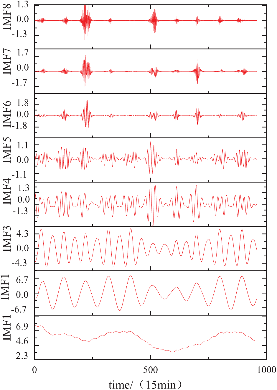
Figure 6: Plot of VMD decomposition results for the intercepted section
As the number of IMF components generated after modal decomposition is too large and predicting them one by one will result in too large a prediction, the reconstructed distributed PV power is predicted by calculating the cosine correlation of each IMF component with the historical power generation data, combining the highly correlated IMF components, and removing the IMF components with low correlation to obtain the reconstructed distributed PV power. The cosine correlation of the IMF components with the cosine correlation of historical distributed PV power is shown in Table 2.

5.3 Evaluation Indicators of Model Effectiveness
A single evaluation index does not reflect the model quality well. Therefore, to assess the accuracy of the prediction model put forward in this paper within the realm of distributed PV power prediction. In this paper, three metrics, namely the mean absolute error (MAE), root mean square error (RMSE), and coefficient of determination (R2), as model prediction assessment indicators. Their expressions are as follows:
where: n represents the total number of predicted samples,
5.4 Experimental Results and Analysis
In order to verify the superiority of the prediction method proposed in this paper, this method and other methods are used to predict the examples, respectively. After experiments, this paper uses 2 layers of convolutional layer and 2 layers of pooling layer. 2 layers of a convolutional layer of neurons were 64 and 256, with a convolutional kernel size of 3, the activation function to choose the ReLU function; pooling layer to select the maximum pooling layer, pooling window and the step size is 2; The channel attention mechanism modifies the weights of channels through global average pooling, a two-layer fully connected layer network where the first layer is a compression layer with r = 8 and ReLU activation function, and the second layer is an expansion layer with sigmoid activation function; the number of neurons of BiLSTM is 128; the batch-size is 600, and the epochs are 100 times. Since distributed PV power generation has a strong diurnal cycle, the historical data in terms of days can show the characteristics of PV for one day, this paper adopts the historical meteorological data and the historical power data as inputs to predict the future power output of single and multi-steps in the form of a sliding window.
First, the effect of adding the VMD decomposition algorithm on improving prediction accuracy is verified. The new dataset reconstructed by the VMD decomposition process and the original dataset without decomposition are input into the CNN-SENet-BiLSTM network, respectively, and the same inputs are used for the algorithms to compare the prediction results. The prediction model which is set to include VMD is set to Model1, and the model which is directly predicted without decomposition is set to Model2. The evaluation metrics are shown in Fig. 7, and the waveform plots of the predicted and true values are shown in Fig. 8.

Figure 7: Impact of VMD decomposition on assessment indicators
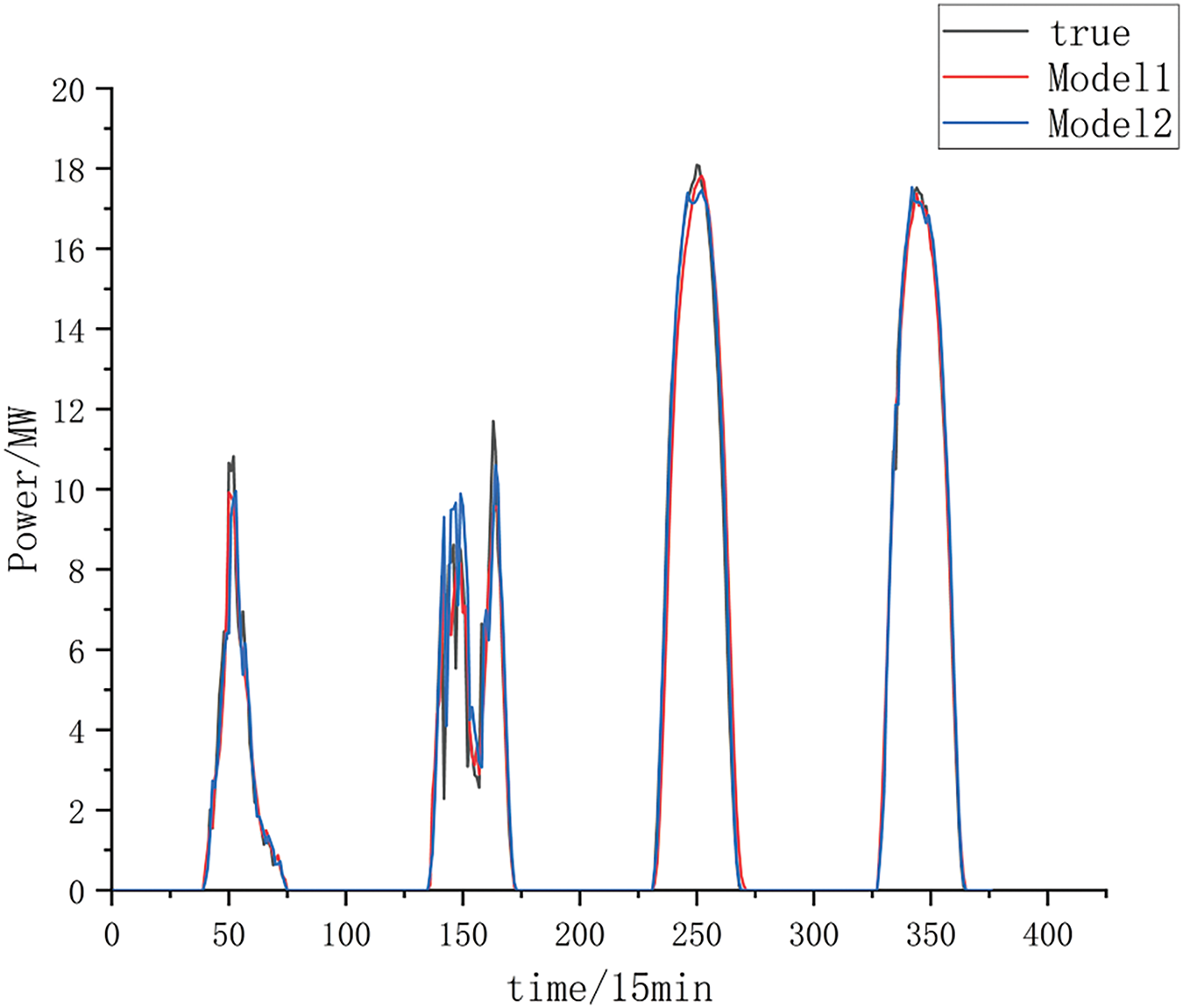
Figure 8: Plot of decomposed and undecomposed prediction results by VMD
As shown in Figs. 7 and 8, the VMD-treated dataset improves the prediction results. The prediction result evaluation metrics MAE, RMSE, and R2 after VMD processing are compared with those without VMD processing, in which MAE is reduced by 16%, RMSE is decreased by 4%, and R2 is increased by 2%. Secondly, the effectiveness of the proposed CNN-SENet-BiLSTM model in enhancing single-step and multi-step prediction accuracy is systematically evaluated. The model put forward in this paper is contrasted with CNN, CNN-LSTM and CNN-BiLSTM, respectively. Where the method proposed in this paper is Model1, CNN is Model2, CNN-LSTM is Model3, and CNN-BiLSTM is Model4 in Fig. 9. The evaluation indices for the single-step prediction of each model are presented in Fig. 9, while the overall prediction outcomes are depicted in Fig. 10.

Figure 9: Changes in evaluation metrics for single-step predictions of different models

Figure 10: Plot of results of single-step prediction for different models
As shown in Figs. 9 and 10, Model1 demonstrates superior performance in single-step prediction. The MAE, RMSE, and R2 values for Model1 in single-step prediction are 0.37, 0.93 MW, and 0.96, respectively. Furthermore, the MAE values are reduced by 21%, 9%, and 26% compared to Model2, Model3, and Model4, respectively. The value of MAE is Mean Absolute Error whose lower value suggests that the model is more effective. The value of RMSE is reduced by 19.8%, 2%, and 20.5% compared to Model2, Model3 and Model4, respectively. Where the value of R2 is improved by 3%, 1%, and 4% compared to Model2, Model3, and Model4, respectively. R2 indicates the degree of model fit, the fit of the model is relatively good, but the model in this paper is also improved compared to other models. The combined prediction method proposed in this research shows the slightest error between the predicted and actual values, as well as the highest degree of fitting compared to individual models. This significantly enhances prediction accuracy and reduces prediction errors. The following evaluation metrics for the multi-step prediction of each model are shown in Fig. 11, and the overall prediction results are shown in Fig. 12.
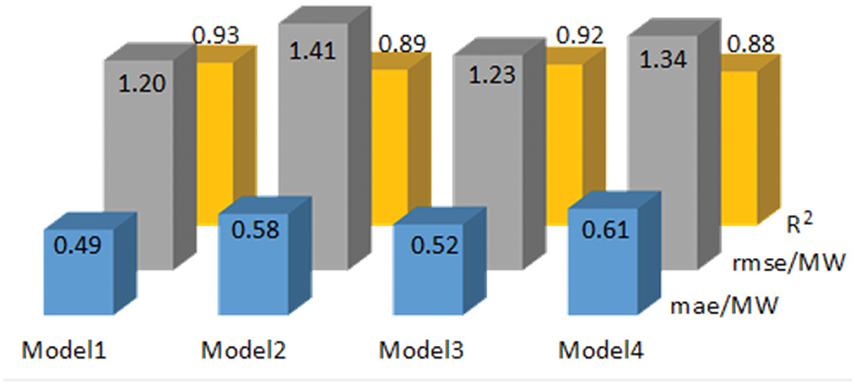
Figure 11: Changes in evaluation metrics for multi-step prediction with different models

Figure 12: Plot of results of multi-step prediction with different models
As shown in Figs. 11 and 12, Model1 demonstrates superior performance in multi-step prediction. The MAE, RMSE and R2 single-step prediction of Model1 are 0.49, 1.20 MW and 0.93, respectively. where the value of MAE is reduced by 15%, 6%, and 18% as compared to Model2, Model3, and Model4, respectively. Where the value of RMSE is reduced by 15%, 2.5%, and 10% compared to Model2, Model3, and Model4, respectively. Where the value of R2 is increased by 4%, 1%, and 4% compared to Model2, Model3, and Model4, respectively. Combining the comparison results of the two algorithms for predicting one day and predicting two days, respectively, it can be seen that compared with CNN, CNN-LSTM, and CNN-BiLSTM. The distributed PV ultrashort-term power prediction method based on the variational modal decomposition with the channel attention mechanism proposed in this paper exhibits a more accurate and stable performance in different time scales.
To further illustrate the superiority of this paper’s model this paper will also compare the changes of indicators between different models and this paper’s model in different seasons. In this paper, the 7-day average data in different seasons are used to evaluate different models, and the evaluation indexes of each model are shown in Table 3. Fig. 13 shows the comparison between the prediction outcomes of various models and their corresponding real-world results for a few days in spring intercepted in this paper.

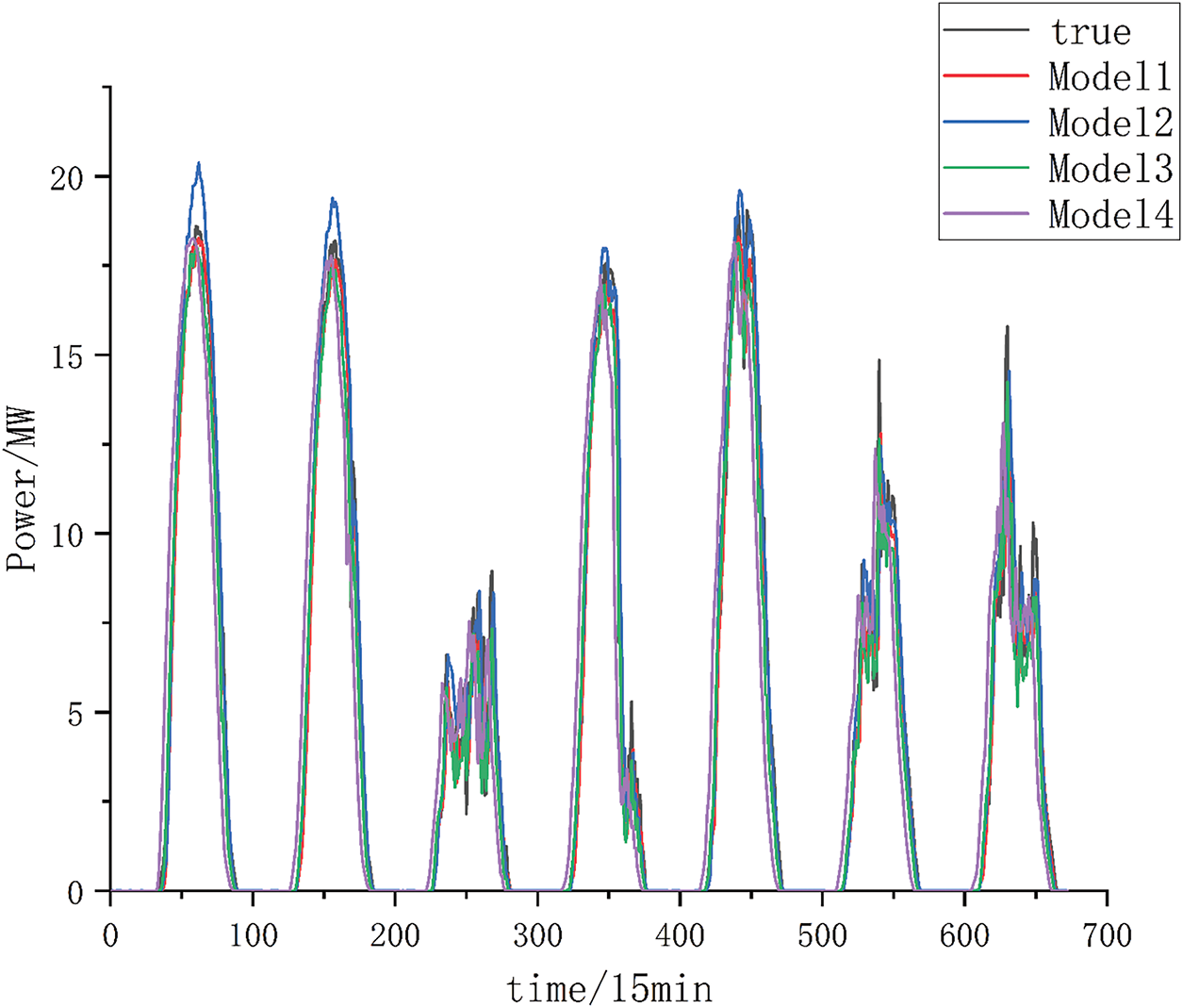
Figure 13: Comparison between the predicted and actual values across different models
As shown in Table 3, Model1 exhibits the smallest mean value across all indices in different seasons. Specifically, the MAE is reduced by 10.8%, 8.8%, and 12.7% compared to the other models, while the RMSE is reduced by 9.2%, 4.3%, and 5.3% compared to the respective models. R2 is improved compared to the rest of the models. In summer and fall, the fit of each model is poorer compared to other seasons, mainly because the weather fluctuations in summer and fall in a region in northwest China are more variable compared to other seasons. As shown in Fig. 13, all models demonstrate higher prediction accuracy during sunny days. During the fluctuating weather, the models face the sudden appearance of the tip value and it is difficult to predict accurately. This kind of weather is one of the main reasons for prediction errors. As can be seen in Fig. 13, Model1 predicted values are more in line with the real values, and the prediction performance is relatively good. In summary, the model introduced in this study still has good prediction performance under different seasons.
To achieve accurate distributed PV power predictions and improve real-time grid scheduling, this paper introduces an ultra-short-term prediction method incorporating variational modal decomposition and a channel attention mechanism. The approach is validated using distributed PV power generation data from a region in northwest China. The main conclusions are as follows:
Making full use of the historical data, the historical power data are decomposed by VMD and sorted according to the magnitude of cosine correlation, and the IMF components with higher correlation are combined to obtain the reconstructed power data. This effectively reduces the complexity of DPV power time series and improves the prediction accuracy of DPV power.
The new dataset composed of reconstructed distributed PV modal components is input into the proposed network, and after the CNN and the channel attention mechanism, the spatial features between the input data can be well extracted, and the key information can also be more prominent.
The spatial features and key information extracted by CNN-SENet are inputted into BiLSTM to complete single-step and multi-step prediction, and finally the prediction results are obtained. Compared with other prediction models, these results are the closest to the real values and have the smallest prediction errors.
In summary, the distributed PV ultra-short-term power prediction method based on variational modal decomposition and the channel attention mechanism proposed in this paper demonstrates high accuracy and stability in PV power forecasting. Furthermore, due to the distributed PV installation policies implemented in China, various regions have integrated a large number of distributed PV resources. The method proposed in this paper provides accurate predictions of distributed PV power, offering valuable guidance for the efficient deployment of distributed PV energy. A significant number of distributed PV resources contribute to the advancement of the national “dual-carbon” policy, effectively reducing China’s carbon emissions. However, this study focuses solely on the prediction of single-distributed PV stations. Considering the decentralized characteristics of regional distributed PV systems, future research should emphasize predicting the output of multiple distributed PV power plants within a region. Different distributed PV power stations, characterized by varying installed capacities, climatic conditions, and geographic locations, highlight the importance of exploring the effects of their synergy and aggregation on prediction accuracy.
Acknowledgement: We are very grateful for the support and cooperation of Northeastern Electric Power University, and thank the editors and reviewers for their valuable comments.
Funding Statement: The study was supported by the Inner Mongolia Power Company 2024 Staff Innovation Studio Innovation Project “Research on Cluster Output Prediction and Group Control Technology for County-Wide Distributed Photovoltaic Construction”.
Author Contributions: The authors confirm contribution to the paper as follows: study conception and design: Zhebin Sun, Wei Wang; data collection: Mingxuan Du, Tao Liang, Yang Liu; analysis and interpretation of results: Mingxuan Du, Hailong Fan, Cuiping Li; draft manuscript preparation: Xingxu Zhu, Junhui Li. All authors reviewed the results and approved the final version of the manuscript.
Availability of Data and Materials: Due to the nature of this research, participants of this study did not agree for their data to be shared publicly, so supporting data is not available.
Ethics Approval: Not applicable.
Conflicts of Interest: The authors declare no conflicts of interest to report regarding the present study.
Nomenclature
| VMD | Variational Mode Decomposition |
| EMD | Empirical Mode Decomposition |
| CNN | Convolutional Neural Network |
| SENet | Squeeze-and-Excitation Networks |
| BiLSTM | Bidirectional Long Short-Term Memory |
| TCN | Temporal Convolutional Network |
| DPV | Distributed Photovoltaic |
References
1. Zhu QF, Li JT, Ji Q, Shi MJ, Wang CL. Application and prospect of artificial intelligence technology in renewable energy forecasting. Proc CSEE. 2023;43(8):3027–48. (In Chinese). doi:10.13334/j.0258-8013.pcsee.213114. [Google Scholar] [CrossRef]
2. Liu Q, Hu Q, Yang LF, Zhou HX. Deep learning photovoltaic power generation model based on time series. Power Syst Prot Control. 2021;49(19):87–98. (In Chinese). doi:10.19783/j.cnki.pspc.201494. [Google Scholar] [CrossRef]
3. National Energy Administration. Installed solar capacity in China [Internet]. Beijing, China: New Energy Cloud; 2025 [cited 9 Mar 2025] (In Chinese). Available from: https://sgnec.sgcc.com.cn/renewableEnergy/developmentSituation. [Google Scholar]
4. Amer HN, Dahlan NY, Azmi AM, Latip MFA, Onn MS, Tumian A. Solar power prediction based on artificial neural network guided by feature selection for large-scale solar photovoltaic plant. Energy Rep. 2023;9(Supplment 12):262–6. doi:10.1016/j.egyr.2023.09.141. [Google Scholar] [CrossRef]
5. Zhao M, Li ST, Chen H, Ling M, Chang H. Distributed solar photovoltaic power prediction algorithm based on deep neural network. J Eng Res. 2025 Forthcoming;37(2):2264. doi:10.1016/j.jer.2024.12.013. [Google Scholar] [CrossRef]
6. Dimd BD, Völler S, Midtgård OM, Cali U, Sevault A. Quantification of the impact of azimuth and tilt angle on the performance of a PV output power forecasting model for BIPVs. IEEE J Photovolt. 2024;14(1):194–200. doi:10.1109/jphotov.2023.3323809. [Google Scholar] [CrossRef]
7. Rawat R, Chandel SS. Review of maximum-power-point tracking techniques for solar-photovoltaic systems. Energy Technol. 2013;1(8):438–48. doi:10.1002/ente.201300053. [Google Scholar] [CrossRef]
8. Amer M, Sajjad U, Hamid K, Rubab N. Reliable prediction of solar photovoltaic power and module efficiency using Bayesian surrogate assisted explainable data-driven model. Results Eng. 2024;24(10):103226. doi:10.1016/j.rineng.2024.103226. [Google Scholar] [CrossRef]
9. Wang HS, Zhang YP, Liang J, Liu LL. DAFA-BiLSTM: deep autoregression feature augmented bidirectional LSTM network for time series prediction. Neural Netw. 2023;157(2):240–56. doi:10.1016/j.neunet.2022.10.009. [Google Scholar] [PubMed] [CrossRef]
10. Zhang WQ, Lin Z, Liu XL. Short-term offshore wind power forecasting—a hybrid model based on discrete wavelet transform (DWTseasonal autoregressive integrated moving average (SARIMAand deep-learning-based long short-term memory (LSTM). Renew Energy. 2022;185:611–28. doi:10.1016/j.renene.2021.12.100. [Google Scholar] [CrossRef]
11. Yang XY, Wang SC, Peng Y, Chen JW, Meng ZC. Short-term photovoltaic power prediction with similar-day integrated by BP-AdaBoost based on the Grey-Markov model. Electr Power Syst Res. 2023;215(Pt A):108966. doi:10.1016/j.epsr.2022.108966. [Google Scholar] [CrossRef]
12. Lin GQ, Li LL, Tseng ML, Liu HM, Yuan DD, Tan RR. An improved moth-flame optimization algorithm for support vector machine prediction of photovoltaic power generation. J Clean Prod. 2020;253(10):119966. doi:10.1016/j.jclepro.2020.119966. [Google Scholar] [CrossRef]
13. Meng A, Xu XC, Chen JM, Wang C, Zhou TM, Yin H. Ultra short term photovoltaic power prediction based on reinforcement learning and combined deep learning model. Power Syst Technol. 2021;45(12):4721–8. (In Chinese). doi:10.13335/j.1000-3673.pst.2021.0319. [Google Scholar] [CrossRef]
14. Zhou DX, Liu YJ, Wang X, Wang FX, Jia Y. Research progress of photovoltaic power prediction technology based on artificial intelligence methods. Energy Eng. 2024;121(12):3573–616. doi:10.32604/ee.2024.055853. [Google Scholar] [CrossRef]
15. Tajjour S, Chandel SS. Power generation forecasting of a solar photovoltaic power plant by a novel transfer learning technique with small solar radiation and power generation training data sets [Internet]. Amsterdam, The Netherlands; 2022. doi:10.2139/ssrn.4024225. [Google Scholar] [CrossRef]
16. Ren XY, Zhang F, Zhu HL, Liu YQ. Quad-kernel deep convolutional neural network for intra-hour photovoltaic power forecasting. Appl Energy. 2022;323(2):119682. doi:10.1016/j.apenergy.2022.119682. [Google Scholar] [CrossRef]
17. Liu RH, Wei JC, Sun GP, Muyeen SM, Lin SF, Li F. A short-term probabilistic photovoltaic power prediction method based on feature selection and improved LSTM neural network. Electr Power Syst Res. 2022;210(4):108069. doi:10.1016/j.epsr.2022.108069. [Google Scholar] [CrossRef]
18. Dai YM, Wang YX, Leng MM, Yang XY, Zhou Q. LOWESS smoothing and random forest based GRU model: a short-term photovoltaic power generation forecasting method. Energy. 2022;256:124661. doi:10.1016/j.energy.2022.124661. [Google Scholar] [CrossRef]
19. Hao JH, Liu FG, Zhang WW. Multi-scale RWKV with 2-dimensional temporal convolutional network for short-term photovoltaic power forecasting. Energy. 2024;309(7938):133068. doi:10.1016/j.energy.2024.133068. [Google Scholar] [CrossRef]
20. Agga A, Abbou A, Labbadi M, El Houm Y, Hammou Ou Ali I. CNN-LSTM: an efficient hybrid deep learning architecture for predicting short-term photovoltaic power production. Electr Power Syst Res. 2022;208(1):107908. doi:10.1016/j.epsr.2022.107908. [Google Scholar] [CrossRef]
21. Limouni T, Yaagoubi R, Bouziane K, Guissi K, Baali EH. Accurate one step and multistep forecasting of very short-term PV power using LSTM-TCN model. Renew Energy. 2023;205:1010–24. doi:10.1016/j.renene.2023.01.118. [Google Scholar] [CrossRef]
22. Zhou N, Shang BW, Xu MM, Peng L, Feng G. Enhancing photovoltaic power prediction using a CNN-LSTM-attention hybrid model with Bayesian hyperparameter optimization. Glob Energy Interconnect. 2024;7(5):667–81. doi:10.1016/j.gloei.2024.10.005. [Google Scholar] [CrossRef]
23. Xu YJ, Zheng SF, Zhu QL, Wong KC, Wang X, Lin QZ. A complementary fused method using GRU and XGBoost models for long-term solar energy hourly forecasting. Expert Syst Appl. 2024;254(3):124286. doi:10.1016/j.eswa.2024.124286. [Google Scholar] [CrossRef]
24. Rao Z, Yang ZM, Li JM, Li LF, Wan SY. Prediction of photovoltaic power generation based on parallel bidirectional long short-term memory networks. Energy Rep. 2024;12(10):3620–9. doi:10.1016/j.egyr.2024.09.043. [Google Scholar] [CrossRef]
25. Kong XF, Du XY, Xue GX, Xu ZJ. Multi-step short-term solar radiation prediction based on empirical mode decomposition and gated recurrent unit optimized via an attention mechanism. Energy. 2023;282(22):128825. doi:10.1016/j.energy.2023.128825. [Google Scholar] [CrossRef]
26. Zhao YX, Wang B, Wang S, Xu WJ, Ma G. Photovoltaic power generation power prediction under major extreme weather based on VMD-KELM. Energy Eng. 2024;121(12):3711–33. doi:10.32604/ee.2024.054032. [Google Scholar] [CrossRef]
27. Ma L, Wang LY, Zeng S, Zhao YT, Liu C, Zhang H, et al. Short-term household load forecasting based on attention mechanism and CNN-ICPSO-LSTM. Energy Eng. 2024;121(6):1473–93. doi:10.32604/ee.2024.047332. [Google Scholar] [CrossRef]
28. Hu J, Shen L, Sun G. Squeeze-and-excitation networks. In: Proceedings of the 27th IEEE/CVF Conference on Computer Vision and Pattern Recognition; 2018 Jun 18–23; Salt Lake City, UT, USA. New York, NY, USA: IEEE; 2018. p. 7132–41. doi:10.1109/CVPR.2018.00745. [Google Scholar] [CrossRef]
29. Taheri S, Talebjedi B, Laukkanen T. Electricity demand time series forecasting based on empirical mode decomposition and long short-term memory. Energy Eng. 2021;118(6):1577–94. doi:10.32604/EE.2021.017795. [Google Scholar] [CrossRef]
Cite This Article
 Copyright © 2025 The Author(s). Published by Tech Science Press.
This work is licensed under a Creative Commons Attribution 4.0 International License , which permits unrestricted use, distribution, and reproduction in any medium, provided the original work is properly cited.
 Downloads
 Citation Tools