
 Submit a Paper
 Propose a Special lssue
 Open Access
ARTICLE

Models for Predicting the Minimum Miscibility Pressure (MMP) of CO2-Oil in Ultra-Deep Oil Reservoirs Based on Machine Learning
1 Huabei Oilfield Company, PetroChina, Renqiu, 062552, China
2 College of Petroleum Engineering, China University of Petroleum (Beijing), Beijing, 102249, China
* Corresponding Author: Tianfu Li. Email:
(This article belongs to the Special Issue: Integrated Geology-Engineering Simulation and Optimizationfor Unconventional Oil and Gas Reservoirs)
Energy Engineering 2025, 122(6), 2215-2238. https://doi.org/10.32604/ee.2025.062876
Received 30 December 2024; Accepted 19 March 2025; Issue published 29 May 2025
 View Full Text
 Download PDF
Abstract
CO2 flooding for enhanced oil recovery (EOR) not only enables underground carbon storage but also plays a critical role in tertiary oil recovery. However, its displacement efficiency is constrained by whether CO2 and crude oil achieve miscibility, necessitating precise prediction of the minimum miscibility pressure (MMP) for CO2-oil systems. Traditional methods, such as experimental measurements and empirical correlations, face challenges including time-consuming procedures and limited applicability. In contrast, artificial intelligence (AI) algorithms have emerged as superior alternatives due to their efficiency, broad applicability, and high prediction accuracy. This study employs four AI algorithms—Random Forest Regression (RFR), Genetic Algorithm Based Back Propagation Artificial Neural Network (GA-BPNN), Support Vector Regression (SVR), and Gaussian Process Regression (GPR)—to establish predictive models for CO2-oil MMP. A comprehensive database comprising 151 data entries was utilized for model development. The performance of these models was rigorously evaluated using five distinct statistical metrics and visualized comparisons. Validation results confirm their accuracy. Field applications demonstrate that all four models are effective for predicting MMP in ultra-deep reservoirs (burial depth >5000 m) with complex crude oil compositions. Among them, the RFR and GA-BPNN models outperform SVR and GPR, achieving root mean square errors (RMSE) of 0.33% and 2.23%, and average absolute percentage relative errors (AAPRE) of 0.01% and 0.04%, respectively. Sensitivity analysis of MMP-influencing factors reveals that reservoir temperature (TR) exerts the most significant impact on MMP, while Xint (mole fraction of intermediate oil components, including C2-C4, CO2, and H2S) exhibits the least influence.Keywords
In recent years, the rapid growth of the global economy has driven a steady rise in demand for oil resources across nations [1]. However, conventional oil recovery methods often exhibit low extraction efficiency, prompting heightened interest in technologies capable of enhancing hydrocarbon recovery [2]. Among these, CO2 flooding stands out as a highly effective and economically viable enhanced oil recovery (EOR) technique. Its significance stems not only from its ability to achieve carbon capture, utilization, and storage (CCUS)—thereby contributing to the mitigation of the greenhouse effect—but also from its cost-effectiveness and operational efficiency [3–5]. The mechanisms by which CO2 enhances oil recovery primarily include viscosity reduction through dissolution into crude oil, interfacial tension reduction, and most critically, miscible or immiscible displacement achieved via compositional interactions with the crude oil. When CO2 is miscible with crude oil, the oil recovery rate will be greatly improved, and theoretically, the displacement efficiency can reach 100% [6].
Related experimental studies and field practices [7,8] have demonstrated that oil recovery rates under miscible and immiscible conditions exhibit marked disparities. Therefore, accurate determination of the minimum miscible pressure (MMP)—the critical threshold delineating miscible and immiscible regimes—is crucial for improving oil recovery efficiency. At present, the main methods for determining the minimum mixed phase pressure include experimental methods, empirical formulas, specific correlations, and intelligent algorithms.
The experimental determination of the MMP is widely adopted in CO2 flooding projects due to its high accuracy and precision. Currently, commonly used experimental methods for determining the MMP include capillary tests, the bubble apparatus method, and the interfacial tension elimination method [9–11]. Although these experimental techniques exhibit high reliability, they are associated with limitations such as time-consuming procedures, high operational costs, and complex operating procedures [12]. Given these constraints, developing rapid and inexpensive method methods for CO2-oil MMP estimation is imperative. Table 1 summarizes prior studies investigating MMP under diverse conditions using experimental and empirical approaches.
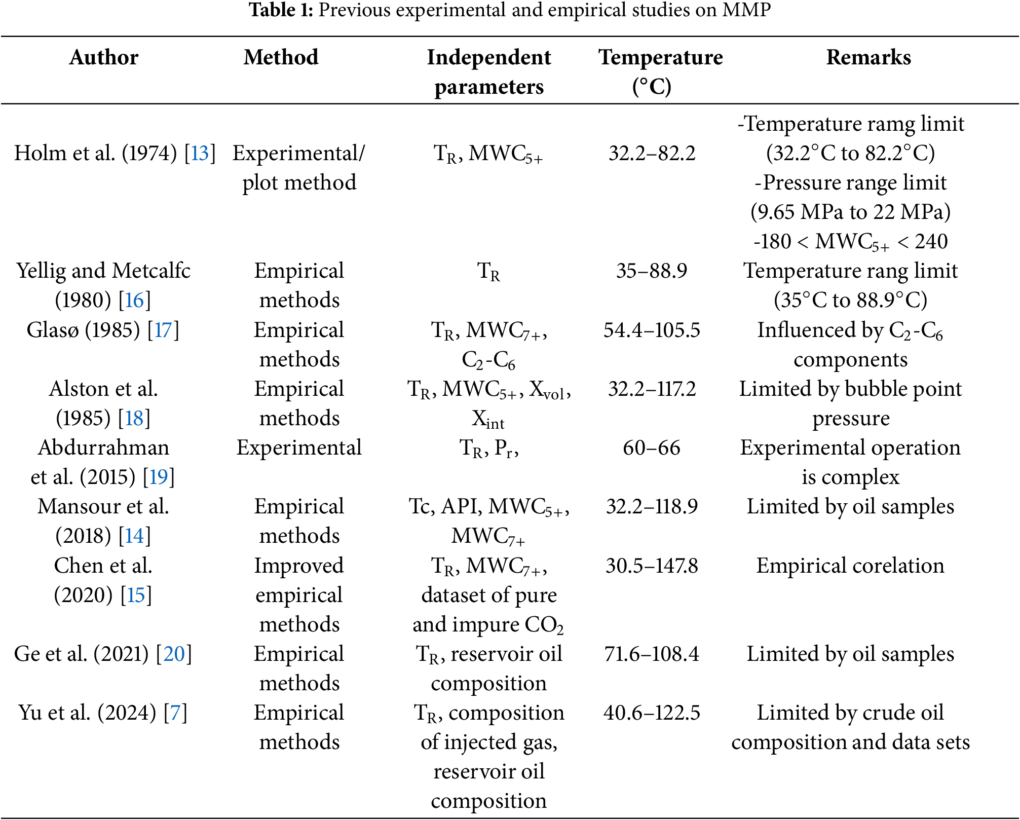
Due to the limitations of experimental methods and the need for rapid prediction of the MMP, various empirical approaches have been proposed, demonstrating significant applicability and gradually emerging as alternatives to traditional experimental techniques. For instance, Holm et al. [13] introduced the plate method for MMP estimation, which relies on analyzing changes in crude oil density within reservoir formations. However, this method is restricted to reservoirs with temperatures between 32.2°C and 82.2°C and formation pressures ranging from 9.65 to 22 MPa. Mansour et al. [14] developed an empirical formula that integrates TC, API, MWC5+, and MWC7+ to predict MMP for live oil systems. Similarly, Chen et al. [15] proposed a multi-factor empirical model accounting for ten variables influencing MMP, which exhibits superior accuracy compared to earlier formulations. Despite these advancements, empirical formulas often suffer from narrow applicability, being valid only for reservoirs with specific characteristics and failing to generalize across diverse geological settings. Consequently, there is a pressing need to develop more accurate and universally adaptable methods for CO2-oil MMP prediction.
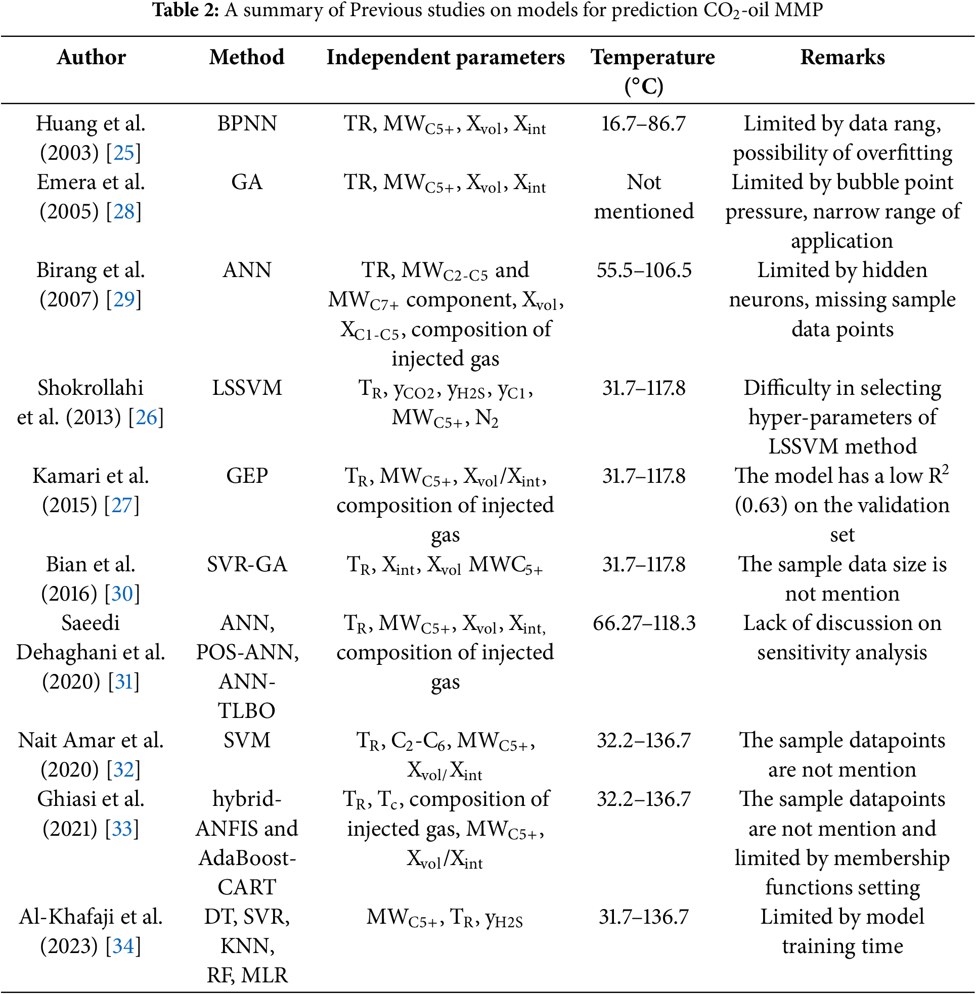
Recent advancements in artificial intelligence (AI), particularly its superior machine learning (ML) capabilities and robust data analytics proficiency, have catalyzed the increasing adoption of ML techniques to address complex challenges in oilfield production. Key applications spanning well-test interpretation, log analysis, reservoir classification, production performance forecasting, and gas solubility prediction in crude oil have demonstrated the efficacy of ML-driven approaches, showcasing their adaptability and precision in handling datasets [21–24]. Given these successes, researchers are now actively exploring ML-based frameworks to predict the CO2-oil MMP. Huang et al. [25] developed a three-layer back propagation artificial neural network(BPNN) model and comprehensively considered the effects of Molecular weight of C5+ fraction, reservoir temperature, and volatility to predict pure and implied CO2-oil MMP. Shokrollahi et al. [26] developed a Least Squares Support Vector Machine model (LSSVM) that comprehensively considers the effects of reservoir temperature, MWC5+, and the contents of yCO2, yH2S, yC1, and N2 in the injected gas to predict pure and impure MMP. Kamari et al. [27] developed a Genetic expression Programming (GEP) model to predict pure and impure CO2-oil MMP in live reservoir oil systems during CO2 flooding. Table 2 provides a comparative summary of predictive models for the CO2-oil MMP developed in previous studies, detailing their input variables and methodological constraints.
The results of these machine learning models for predicting MMP indicate that reservoir temperature and crude oil composition have significantly impact on MMP [21,23,24,26,27]. For ultra-deep oil reservoirs buried deeper than 5000 m, characteristics such as high reservoir temperature and complex crude oil composition are present. Existing prediction models exhibit low accuracy and local overfitting problems when predicting MMP in ultra-deep oil reservoirs. In order to quickly and accurately predict MMP in ultra-deep oil reservoirs, we developed multiple models with ten input parameters (i.e., TR, Xvol, Xint, XC5-C6, MWC7+, mole fraction of CO2 in solution (yCO2), mole fraction of C1 in the CO2 injection gas (yC1), mole fraction of N2 in the injection gas (yN2), mole fraction of H2S in the injection gas (yH2S), and mole fraction of C2-C4 in the injection gas (yC2-C4)) to predict MMP in both pure and impure CO2 injection cases in ultra-deep oil reservoirs. Based on the above description, multiple models were established and optimized, and suitable model for CO2 MMP in ultra-deep oil reservoirs was selected by comparing the prediction results of different models. Grid search was employed to tune and optimize the hyperparameters of these models, which predict the CO2-oil MMP in ultra-deep oil reservoirs, thereby ensuring their predictive accuracy. In addition, a sensitivity analysis was systematically conducted to quantify the relative contributions of individual factors affecting MMP and to elucidate the functional dependencies of MMP on these critical variables.
2 Minimum Miscibility Pressure (MMP)
During the process of injecting CO2 into oil reservoirs for enhanced oil recovery, interactions between gas, oil, and water phases occur in the rock layers, resulting in interphase component transfer, phase transitions, and other complex phase behaviors. CO2 undergoes multiple contact displacements with crude oil under reservoir temperature and pressure, achieving either miscible or immiscible flooding. The CO2 mixed-phase drive refers to the formation of a stable mixed-phase zone at the leading edge between CO2 and crude oil when the injection pressure is higher than a certain value and the disappearance of the oil-gas interface, resulting in zero interfacial tension in porous media. This pressure is called the minimum miscibility pressure.
It is widely recognized that temperature, crude oil components, and the composition of injected gas significantly influence the MMP. To date, researchers [27,30,31,33] have conducted comprehensive studies on the influencing factors affecting MMP. Reservoir temperature plays a crucial role in the MMP during CO2 flooding. As the reservoir temperature increases, the amount of CO2 dissolved in crude oil decreases, and the supercritical nature of CO2 diminishes, particularly in terms of density. This reduction seriously affects the ability of CO2 extraction to extract light hydrocarbons. Currently, most research indicates a linear positive correlation between CO2-oil MMP and reservoir temperature. Alston et al. [18] studied the crude oil components, dividing them into three parts—Xvol, Xint, and MWC5+—have an impact on MMP, but MWC5+ has a more significant effect on CO2-oil MMP. Additionally, injecting gas components also has a significant impact on MMP. Sebastian et al. [35] found that injecting CO2 gas containing C1, N2, H2S, and light component hydrocarbons (C2-C4) can have an impact on CO2-oil MMP.
Consequently, ten factors (TR, xint, xvol, xC5–C6, MWC7+, yC1, yN2, yCO2, yC2-C4, and yH2S) that significantly affect MMP were selected as the input variables and imported to design multiple models for MMP simulation. To evaluate the correlation between these characteristic variables and their influence on the MMP, this study employs the partial correlation analysis to detect any redundant information among the variables and ensure their independence. The results are shown in Fig. 1. It can be seen from the Fig. 1 that the r values between any two feature variables and MMP differ, indicating that the ten features are independent of each other and there is no significant collinearity problem.
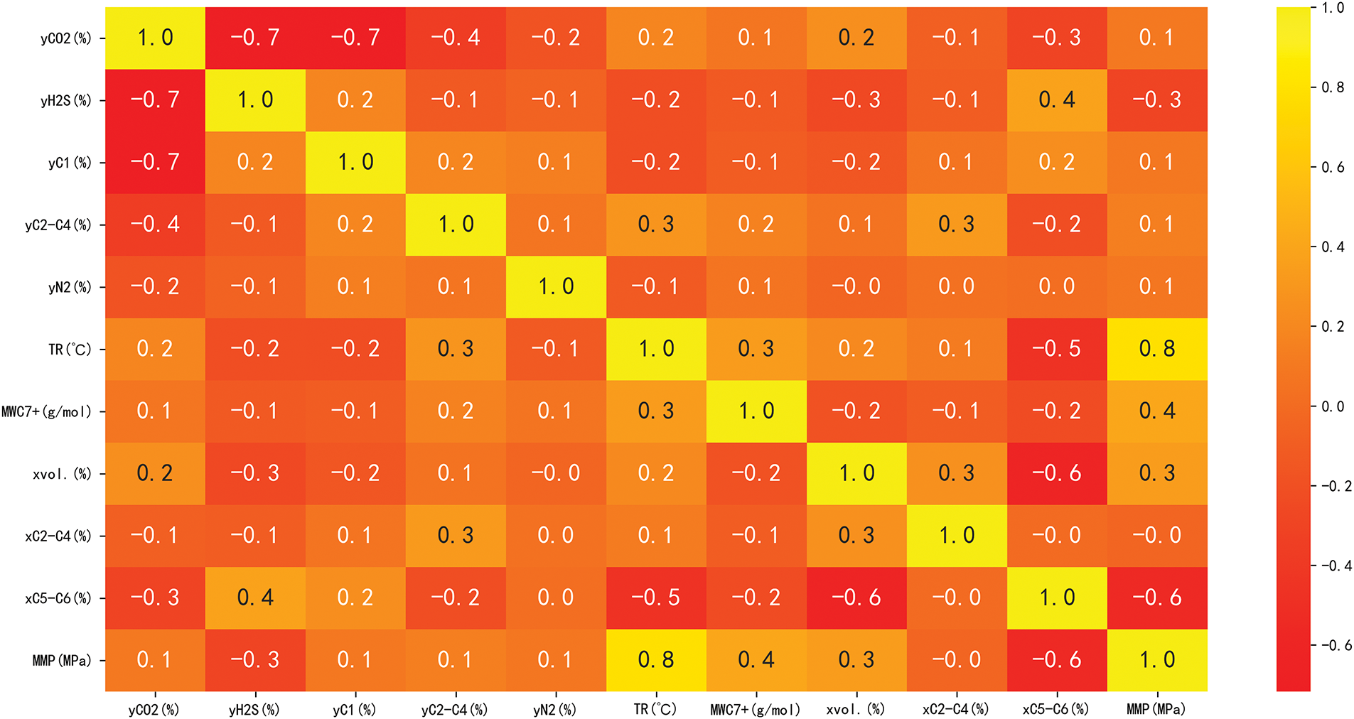
Figure 1: Partial correlation analysis results heatmap
3 Basic Description of Models and Experimental Data
Artificial Neural Networks (ANNs) are computational models designed to simulate the structure and function of neurons in the human brain. Similar to the way the human brain works, artificial neural networks can automatically process multiple input variables in parallel, passing information from the input layer to the output layer through the learning process [36,37]. In addition, ANNs also have the ability to reveal potential linear or nonlinear relationships between input and output data. A complete neural network consists of an input layer, an output layer, and at least one hidden layer. The basic structural unit of a neural network is the neuron, which can receive, process, and output signals. It is a nonlinear element with multiple inputs and a single output. A large number of neurons are interconnected via connection weights, bias values, and transfer functions between neurons in each layer, forming a neural network with robust information processing capabilities. A back propagation neural network (BPNN) is a type of feedforward neural network that incorporates a backpropagation learning algorithm. Due to its adjustable architecture, capability for forward signal propagation, and mechanism of error backpropagation, the BPNN has emerged as the most widely implemented neural network paradigm. The schematic architecture of a standard three-layer BPNN is depicted in Fig. 2. However, ANN models are prone to challenges, including overfitting, suboptimal parameter selection, and computational inefficiency during training. To mitigate these limitations, a hybrid framework integrating a Genetic Algorithm (GA) and BPNN is employed to optimize network weights and biases, thereby enhancing prediction accuracy [38].
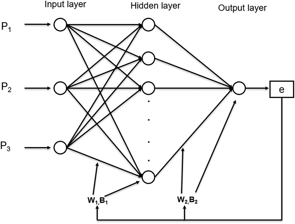
Figure 2: Typical three-layer backpropagation neural network model structure diagram
The GA, first proposed by American scholar John Holland, it a global optimization algorithm that simulates the process of biological evolution.GA mimics principles of natural selection, crossover, and mutation to enhance individual fitness within a population. Its workflow comprises four stages: parameter encoding, population initialization, fitness evaluation, and iterative genetic operations [39,40]. Genetic operations include selection, crossover, and mutation. The selection operation can inherit excellent chromosomes to the next generation or generate new individuals through crossover operation and pass them on to the next generation. By adopting an optimal preservation method, the fitness values of individuals within the same population are sorted in descending order, with priority given to selecting individuals with higher fitness values for inheritance to the next generation. The crossover operation is the process of selecting chromosomes from a population and recombining them into new chromosomes through crossover operations. This operation can effectively inherit excellent genes from the population. The mutation operation involves using other genes in an individual to replace specific genes, which can enhance local search ability and effectively preserve population diversity. In general, selection operations ensure that the population evolves toward higher fitness, crossover operations accelerate the speed of genetic algorithm searching for optimal solutions, and mutation operations help prevent the algorithm from falling into local optima too early. Together, the three genetic operations of selection, crossover, and mutation enable GA to efficiently search the solution space and gradually approach the optimal solution.
Optimizing the BPNN model through GA and developing the GA-BPNN hybrid model. The specific steps are as follows:
(1) Initialization: Define the BPNN architecture and initialize GA parameters and population.
(2) Fitness Evaluation: Train the BPNN on the dataset and calculate individual fitness based on prediction accuracy.
(3) GA Execution: Perform selection, crossover, and mutation operations within the GA.
(4) Population Update: Replace old individuals with newly generated individuals to form a new population.
(5) Termination Check: Determine whether the termination condition is satisfied. If the termination condition is not satisfied, return to step 2 to continue the iteration.
(6) Model Finalization: Deploy the BPNN with optimized weights and biases from the highest-fitness individual.
RFR is an ensemble algorithm composed of multiple decision trees based on the bootstrap aggregating method; it was initially designed for classification tasks. As research progressed, the RFR model was further applied to predict CO2-oil MMP. For instance, Al Khafaji et al. [34] used the RFR model to predict MMP. The basic principles of RFR can be summarized as four steps: sample selection, feature selection, decision tree construction, and prediction. The number of trees in a random forest is represented as B, and the predicted result of the b-th tree is represented as Fb(x). Therefore, the prediction formula for RFR can be expressed as:
The steps for establishing a random forest regression model are as follows:
(1) Data Standardization: Standardize all data to ensure that their values are between –1 and 1, in order to obtain accurate prediction results and accelerate training speed.
(2) Import Data and Select Parameters: Import all data and output the dataset to the model for model training and testing.
(3) Bootstrap Sampling: The bootstrap resampling method is employed to randomly sample the original dataset with replacement, generating multiple subsets. Each subset trains a decision tree, while the unsampled instances (termed out-of-bag (OOB) data) are reserved for validation.
(4) Tree Growth: Each decision tree randomly selects several features from the input variable x for the current node’s split subset. The optimal feature for splitting is determined by maximizing variance reduction, which enables maximal tree growth.
(5) OOB Validation: The OOB data, which are excluded from the training process, serve to evaluate model performance and accuracy. The optimal number of decision trees, T, is determined by iteratively refining the model based on OOB prediction errors until convergence.
(6) Prediction: For the input variable xi (i = 1, 2, … , k) that needs to be predicted. Each decision tree will output a corresponding predicted value yi (i = 1, 2, … , k).The predicted value of RFR is the average of the predicted values of all decision trees.
SVR is a regression analysis method derived from Support Vector Machines (SVM). While SVR shares conceptual similarities with traditional SVM classification algorithms, its objective diverges by focusing on identifying an optimal fitting function for continuous prediction problems, as opposed to delineating classification boundaries [41]. The basic idea of the SVR model is to find a function that can predict the output value as accurately as possible while keeping the complexity of the model low to avoid overfitting. To achieve this goal, SVR uses a loss function called “ε-insensitive loss function”, which means that the loss is only calculated when the prediction error exceeds a certain threshold, ε [42]. Its basic definition is as follows:
In the nonlinear case, by introducing relaxation variables
The model is subject to the following constraints:
The solution to this problem can be achieved by introducing Lagrange functions
where,
The constraints imposed on the SVR model are as follows:
where,
Based on the above analysis, obtain the optimal solution and derive the final regression function:
where,
The steps for establishing a support vector machine regression model are as follows:
(1) Read and preprocess the dataset.
(2) Build a model and define a hyperparameter search space.
(3) Use grid search cross-validation to find the optimal hyperparameters.
(4) Train the model using the optimal hyperparameters and conduct model evaluation.
(5) Use the trained model to predict new input data and output the prediction results.
3.4 Gaussian Process Regression
GPR is a data-driven method proposed by Williams and Rasmussen. Its essence lies in learning the kernel function with probabilistic significance [43]. The optimal hyperparameters are obtained by analyzing historical sample data, after which a prediction model is developed to forecast subsequent samples. The prediction generated by the GPR method carry probabilistic significance and can describe associated with these predictions. Compared with ANN, SVR and other methods, the hyperparameters required for prediction are easier to obtain and are suitable for high-dimensional nonlinear systems. Fig. 3 illustrates the specific process of GPR. The GPR algorithm is described below.
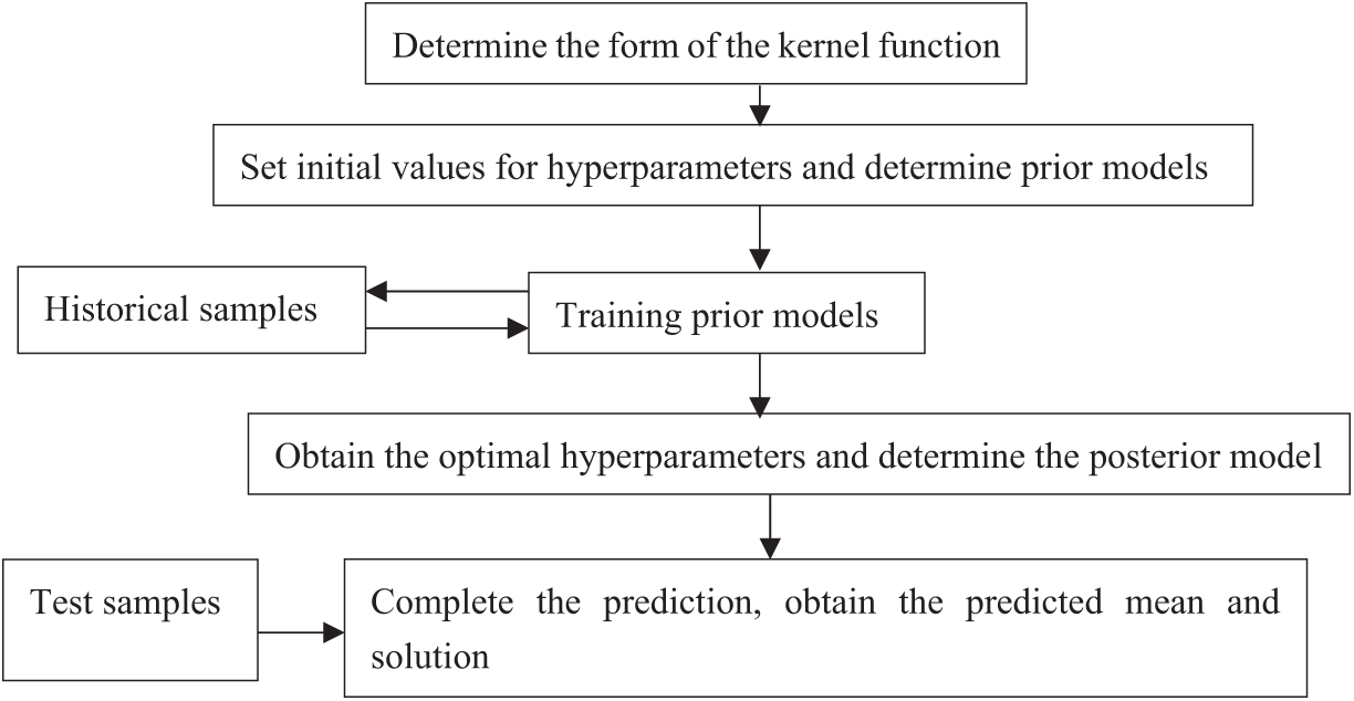
Figure 3: Process of GPR
Given the training set D:
where, Xm and Xn represent the m-th and n-th vectors,
The most widely used covariance function is:
where, L represents the number of elements in vector Xi,
For a new input vector XN+1, use a predictive model to estimate its tN+1 value rate distribution, expectation, and variance are used for prediction, and the model function is represented as:
where, y(Xn) represents modeling functions,
So the model probability is:
where, P(y|A) is the pre probability distribution of y(x), A is a set of hyperparameters of P(y|A), P(
Let TN = (t1, t2, … , tn), TN+1 = (t1, t2, … , tn, tn+1), therefore the conditional distribution of tN+1 can be represented by Eq. (13), and it can be used to predict tN+1:
According to Bayesian method, it can be inferred that the distribution function of tN+1 is:
By substituting the Gaussian distribution formula, the preliminary calculation can be simplified as:
where, ZN and ZN+1 are two normalization constants.
After further simplification, the following equation can be obtained:
where,
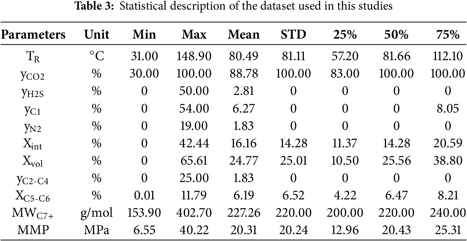
The predictive reliability and accuracy of machine learning models are critically contingent upon the representativeness and robustness of the training dataset. In the frameworks of ANN, RFR, GPR, and SVR, input data are conventionally partitioned into training and testing subsets. The former serves to calibrate model parameters and optimize predictive performance, whereas the latter is employed to assess the accuracy and stability of the models.
The experimental dataset employed in this investigation comprises 151 data entries, partitioned into two categories: 89 records of pure CO2 injection and 62 records of impure CO2 injection. The dataset was divided into training (90%, n = 136) and testing (10%, n = 15) subsets to ensure unbiased model validation. These data were collected from various mature experimental works in the literature [13,15,44,45]. Data sets include experimental values for reservoir temperature, composition of drive gas (yCO2, yH2S, yN2, and yC2–C4), molecular weight of the C7+ fraction in crude oil (MWC7+), the ratio of volatile (Xvol) to intermediate (Xint) components in crude oil, pure and impure CO2-oil MMP. Table 3 presents a statistical description of the dataset used. A detailed analysis of the experimental data highlights that the reservoir temperature ranges from 31.00°C to 148.90°C, the experimental values for MMP range from 6.55 to 40.22 MPa.
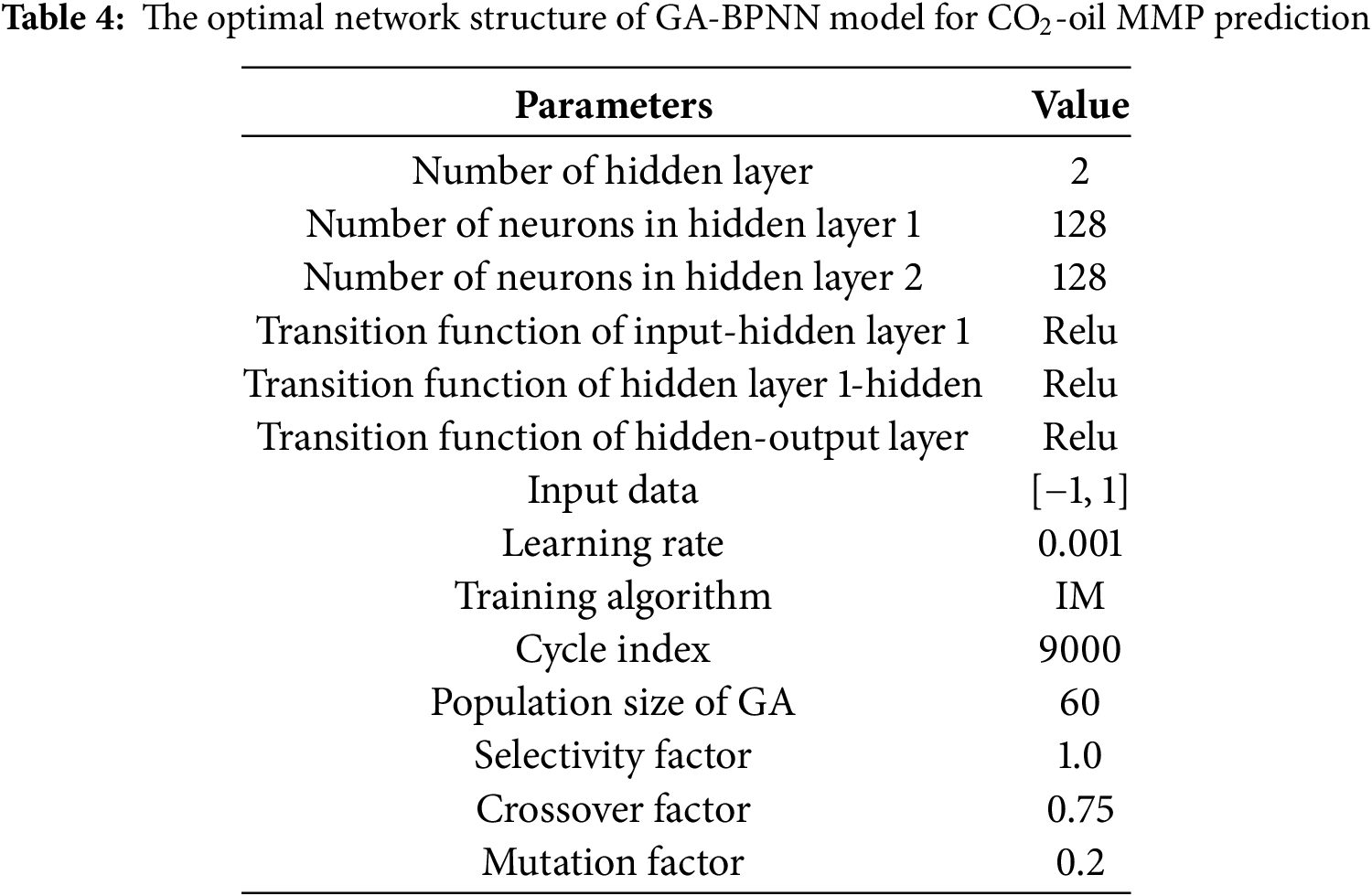
In this study, we have researched and implemented four intelligent algorithm technologies, including GA-BPNN, RFR, GPR and SVR, and established an accurate and stable MMP prediction model. The optimal configuration of the GA-BPNN model is obtained through trial and error. Table 4 shows the optimal network structure of the GA-BPNN model for CO2-oil MMP prediction. All models are written and implemented in Python.
To significantly demonstrate the predictive performance of each model, four statistical error functions were selected to evaluate the performance of the models: the coefficient of variation (CV), absolute percent relative error (APRE), average absolute percent relative error (AAPRE), and root mean square error (RMSE). The closer the value is to 0, the higher the accuracy of the model. Additionally, the coefficient of determination (R2) is also used as the regression evaluation index, and the closer R2 is to 1, the better the fitting effect. The specific calculation methods for the four statistical error functions are as follows:
where,
4.1 Comparison between Different Models
In this section, we will statistically analyze the values of four statistical error functions, with Table 5 displaying the implementation performance of each model. In this table, the performance of the training and the testing data is listed separately. From Table 5, it can be observed that the RFR model has R2 values close to 1 compared to the other three models on both the training and testing sets, specifically are 0.98 and 0.95, respectively. The MAPE and RMSE values on the testing set are also quite low, at 4.31% and 1.00%, respectively. These indicators suggest that the RFR model exhibits the highest prediction accuracy and strong stability. Besides, the GA-BPNN model demonstrates good prediction performance, ranking second to RFR. In comparison, it is evident that GPR has the lowest performance among the four models.
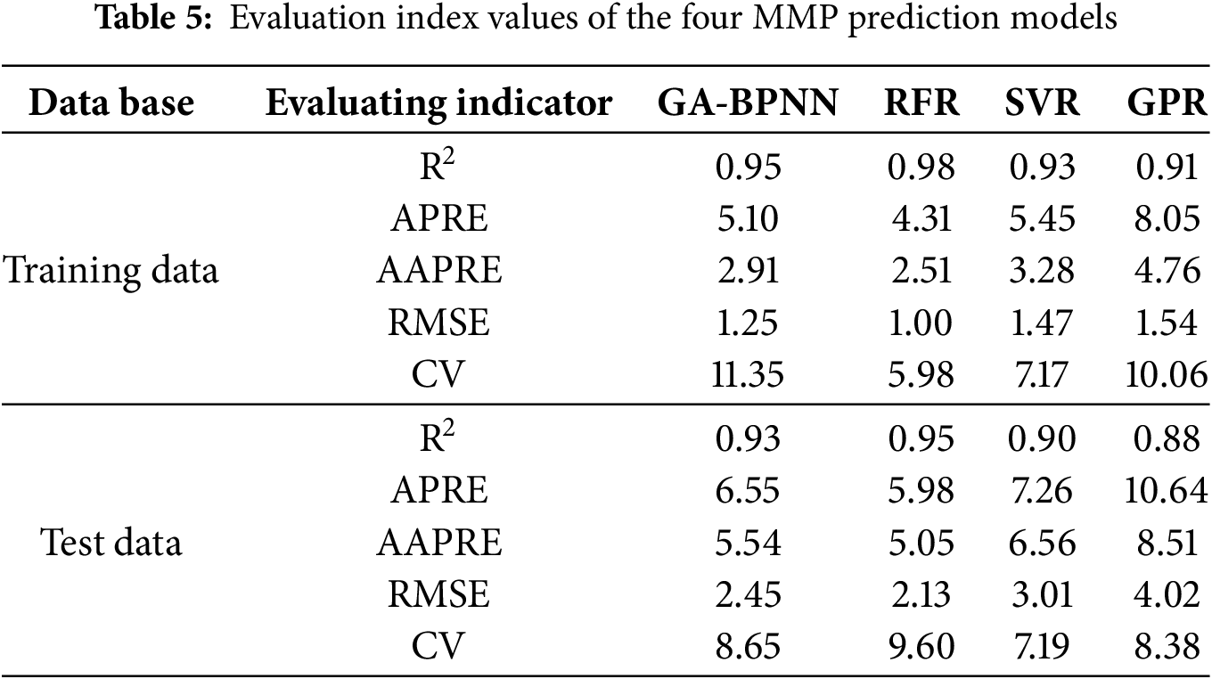
Among the four models evaluated, the RFR operates under the ensemble learning paradigm, which aggregates predictions from multiple decision trees to mitigate overfitting and enhance generalization. This method has obvious advantages over neural networks in processing small and medium-sized data sets (<10,000 samples).The GPR model is distinguished by kernel flexibility. By selecting the appropriate covariance function, GPR can adapt to different data structures (periodic/non-periodic), and provide probability output to quantify the prediction uncertainty, which is a very valuable feature for risk perception decision-making in reservoir engineering. However, GPR 's dependence on computationally intensive hyperparameter optimization often leads to local optimum, especially in high-dimensional parameter space, so advanced global optimization techniques such as Bayesian optimization are needed. Due to its ε-insensitive loss function, SVR is theoretically robust to outliers and noise, and can ignore the error within the tolerance threshold. Its performance depends heavily on the choice of kernel functions (e.g., linear, polynomial) and hyperparameter tuning, but it has interpretability defects and sensitivity to parameter initialization. The predictive performance of the neural network model in this study was not outstanding, and the BPNN algorithm optimized with GA did not demonstrate its outstanding predictive ability. It is speculated that this may be due to the lack of massive data in related research fields, and the big data fitting advantage of the GA-BPNN model has not been fully utilized.
To better illustrate the model performance, Fig. 4 displays the MMP data predicted by RFR, GA-BPNN, SVR, and GPR models. From Fig. 4, it can be seen that the RFR, GA-BPNN, and SVR models have achieved good alignment near the unit slope compared to the GPR model. Among the four models, the error distribution of the RFR and the GA-BPNN models is relatively balanced, with fewer outliers, thus ensuring good stability. The error visualization of the GPR model around the unit slope is quite evident, but it remains within an acceptable range.
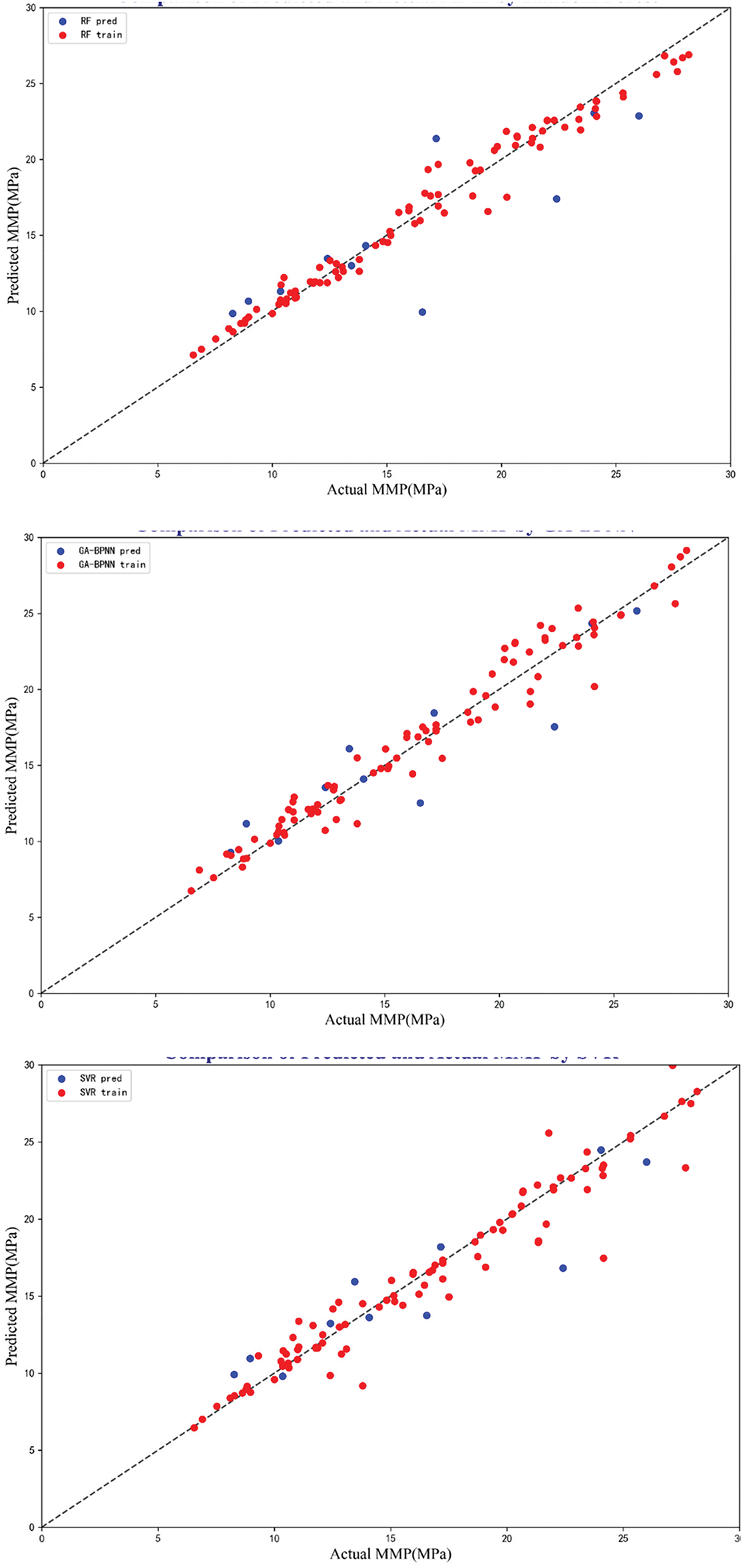
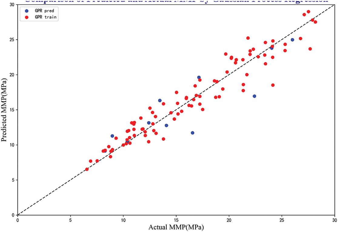
Figure 4: Prediction performance of four models
4.2 Comparison Models with Correlations from Literature
To further validate the predictive performance of the model, a statistical error analysis will be conducted based on previous models. The prediction results of the RFR model and GA-BPNN model developed in this paper will be compared with six forecasting MMP methods proposed by Lee [46], Cronquist [47], Yellig and Metcalfc [16], Alston et al. [18], Emera et al. [28], and Yuan et al. [48]. The six comparative models selected in this article simultaneously consider the influence of CO2 injection gas impurities on the prediction results of CO2-oil MMP, as well as the influencing factors of MMP prediction under pure CO2 injection. Therefore, they were used for comparison with RFR and GA-BPNN models.
Fig. 5 visually displays the comparison results between the simulated MMP values and literature methods. The unit slope line in Fig. 5 serves as the evaluation criterion; the closer the data points are to the unit slope line, the higher the consistency between the simulated and experimental values. Table 6 shows the comparison of various indicators of the model. These results indicate that the RFR model and GA-BPNN model have strong predictive abilities.
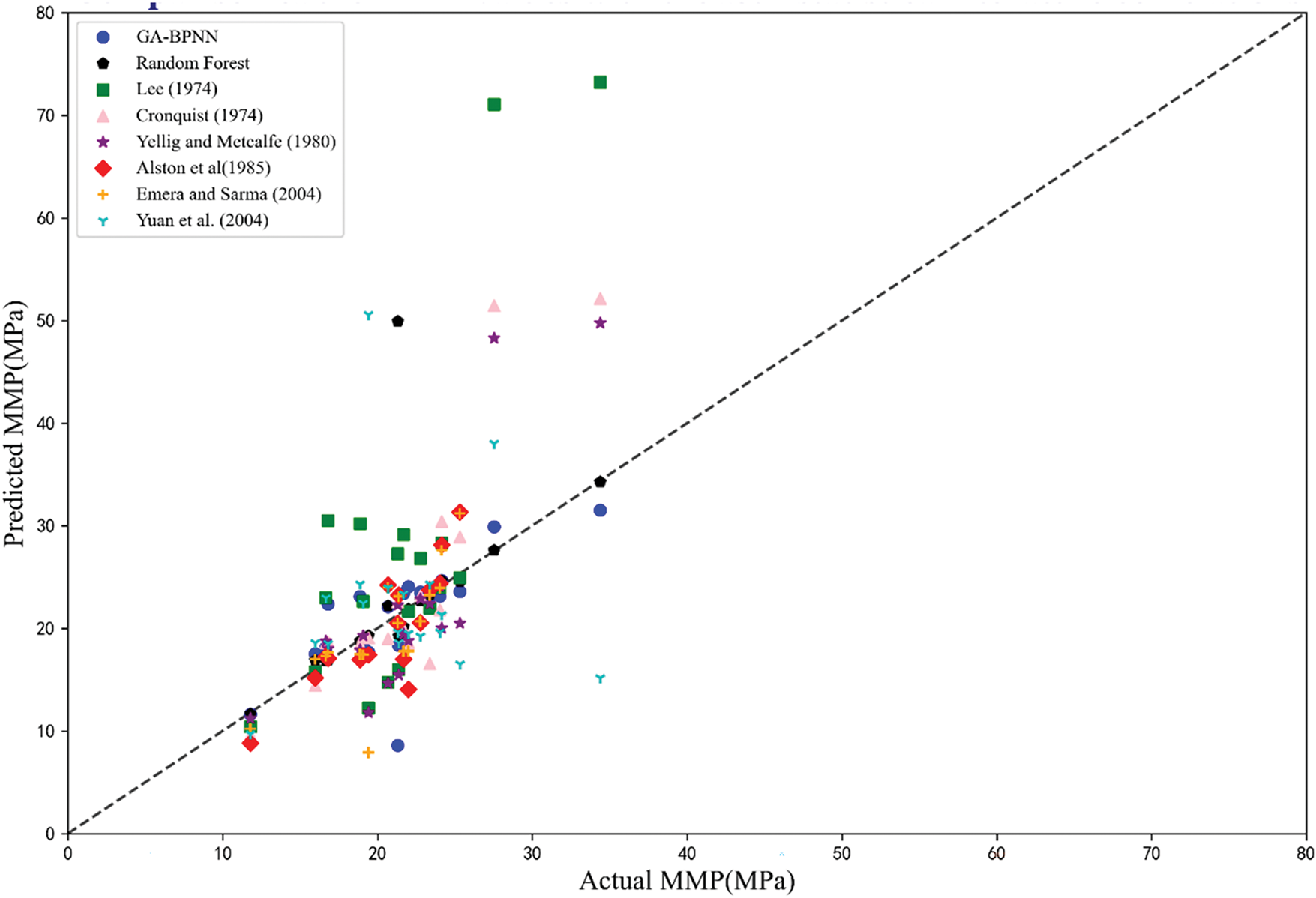
Figure 5: Comparison of the simulated MMP values with that calculated from literature models [16,18,28,46–48]

Analyze the impact of the characteristic parameters of the four models used in this article on predicting MMP in order to deepen our understanding of the CO2-oil interaction mechanism and its intrinsic correlation. In this study, the relevance factor (R) was utilized to assess the extent of influence that each parameter has on MMP. For input variables, the R is a value ranging from −1 to 1. When R is negative, it represents that the input variable has a negative effect on the output variable, and when R is positive, it indicates that the input variable has a positive effect on the output variable. The absolute value of R represents the impact of the input variable on the output variable, and the larger the absolute value of R, the greater the impact of the input variable on the output variable. The calculation formula for R is as follows:
where,
Fig. 6 visually displays the R value of each input variable. From Fig. 6, it can be seen that Xint, XC5-C6, and yH2S can reduce the value of MMP. The observed negative correlations between Xint, XC5-C6, yH2S, and MMP can be attributed to their thermodynamic roles in reducing CO2-oil interfacial tension. The ability of yH2S to reduce MMP is due to the polarity of H2S molecules, which can effectively reduce the interfacial tension between CO2 and oil. The C2-C6 components in crude oil have similar molecular weights and properties to CO2, which helps to increase the solubility of CO2 in crude oil and reduce CO2-oil MMP.
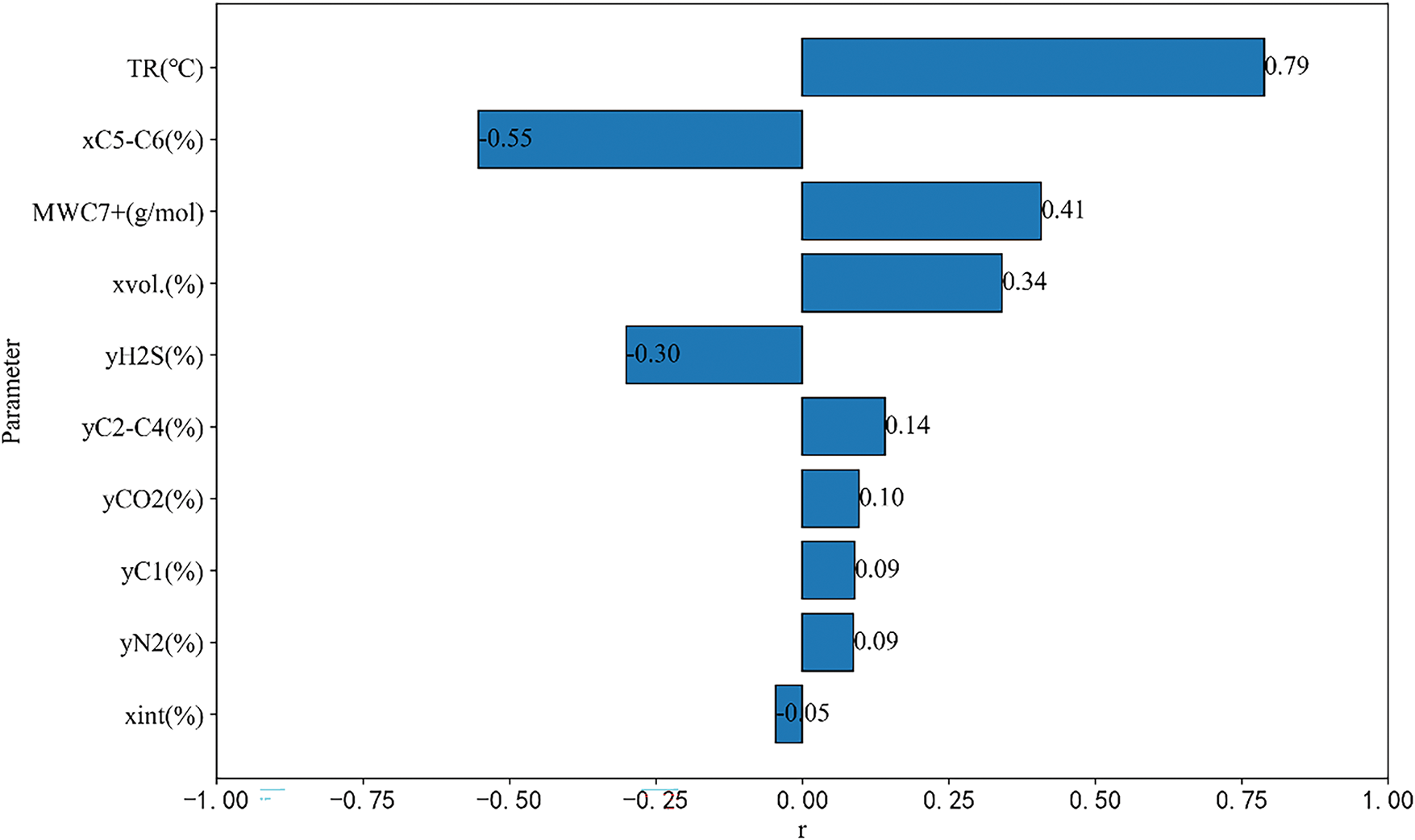
Figure 6: Relevancy factor of input variables on CO2-oil MMP
The increase of the other seven factors (TR, MWC7+, Xvol, yC2-C4, yCO2, yC1, yN2) will lead to an increase in CO2-oil MMP. The increase of TR will result in a decrease in the solubility of CO2 in crude oil, which seriously affects the ability of CO2 extraction to extract light hydrocarbons, ultimately leading to an increase in CO2-oil MMP. An increase of MWC7+ may create a greater difference between crude oil and CO2 molecules, resulting in an increase in interfacial tension and thus affecting MMP. For the light components (Xvol) in crude oil, due to their easy volatilization, they are prone to entering the CO2 gas phase from the crude oil during the CO2 oil multi-stage mixed phase contact process, which results in a decrease in CO2 purity and an increase in MMP. The increase in CO2 concentration enhances the frequency of contact between CO2 and crude oil. As CO2 continuously extracts lighter components from the crude oil, the proportion of heavier components increases. Since these heavier components exhibit poor miscibility with CO₂, a higher pressure is required to achieve miscibility. Within the parameter curve range, the influence of the ten influencing factors on MMP is ranked in descending order: TR > XC5-C6 > MWC7+ > Xvol > yH2S > yC2-C4 > yCO2 > yC1, yN2 > Xint.
4.4 Models Application to Ultra-Deep Oil Reservoir
The Xinghua Block of Bayan oil field is a typical ultra-deep oil reservoir characterized by a large burial depth (>5000 m), high formation temperature and pressure, complex crude oil composition, and intricate fluid phases [49,50]. To verify the applicability of the established CO2-oil MMP prediction models for ultra-deep oil reservoirs, experimental measurement data of CO2 flooding MMP from two wells in Xinghua block of Bayan oil field were selected. The thin tube experiment refers to a simulated displacement test conducted in a thin tube model, and the experimental flowchart is shown in Fig. 7. The criterion for determining whether the thin tube experiment qualifies as a mixed-phase displacement is that the crude oil recovery rate, when injected with 1.2 pore volume(PV) exceeds 90%. Additionally, as the displacement pressure increases, there is no significant rise in displacement efficiency, and mixed-phase fluids can be observed in the observation window. The method for determining MMP is to plot the relationship curve between the recovery degree and displacement pressure when injecting 1.2 PV in each thin tube experiment, while ensuring that the thin tube experiment achieves three cycles of miscible flooding and three cycles of immiscible flooding [51].The pressure corresponding to the intersection of the non-mixed phase and mixed phase curves is the minimum mixed phase pressure (MMP), as shown in Fig. 8. The results of the slim tube test showed that injecting pure CO2 at formation temperatures of 139°C and 133.9°C resulted in MMP values of 49.79 and 48.48 MPa for the reservoir, respectively.
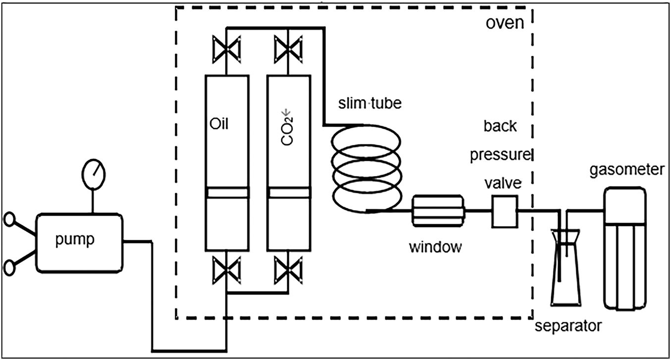
Figure 7: Flow chart of thin tube test
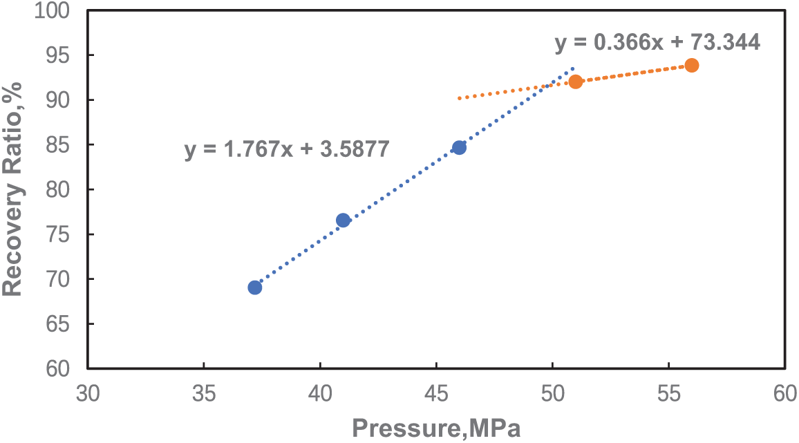
Figure 8: Relationship curve between CO2 displacement recovery degree and displacement pressure in the formation oil slim tube experiment of Bayan oil field
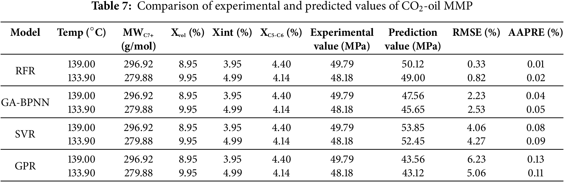
Calculate the MMP using the development prediction models and compare the calculated value with the experimental value measured by the thin tube experiment, Table 7 shows the comparison results between the MMP values predicted by four models and the experimental values measured by capillary experiments. As summarized in Table 7, both the RFR and GA-BPNN models demonstrate superior predictive accuracy, with RMSE values below 3% and AAPRE less than 0.1%. Furthermore, all four models exhibit minimal deviations between predicted and experimentally measured MMP, with errors consistently confined within engineering-acceptable thresholds (relative error < 5%). These results validate the robustness and applicability of the proposed models for MMP prediction in ultra-deep reservoirs characterized by high-temperature, high-pressure conditions.
In this study, we developed four MMP prediction models based on machine learning, namely RFR,GA-BPNN,SVR and GPR. Additionally, we separately investigated pure CO2 gas injection and impure CO2 injection as described in the literature. Across these four models, total of ten impact factors (e.g., TR, xint, xvol, xC5–C6, MWC7+, yC1, yN2, yCO2, yC2-C4, yH2S) were selected, with MMP serving as the output variable. Based on a comprehensive understanding of four models and discussions of the simulation results, the study’s conclusions can be briefly described as follows:
(1) The developed fours models for predicting MMP can effectively predict MMP for both pure CO2 and impure CO2 gas injections, and they can all be utilized for MMP prediction in ultra-deep oil reservoirs.
(2) Among the four models studied in this article, the RFR model exhibits the best predictive performance, while the GPR model shows the worst predictive performance. However, the BPNN algorithm optimized with GA did not demonstrate its outstanding predictive ability, which may be due to its incomplete utilization of the advantages of big data fitting.
(3) In the comparison with experimental results with those from six forecasting MMP methods, the RFR model and GA-BPNN model showed excellent performance.
(4) Among the ten influencing factors studied, Xint, XC5-C6, and yH2S are negatively correlated with MMP, while TR, MWC7+, Xvol, yC2-C4, yCO2, yC1 and yN2 are positively correlated with MMP. Among those, TR has the greatest impact on MMP, followed by XC5-C6 and MWC7+. The degree of influence of the ten influencing factors on MMP, in descending order, is as follows: TR > XC5-C6 > MWC7+ > Xvol > yH2S > yC2-C4 > yCO2 > yC1, yN2 > Xint.
(5) The difference between the properties of crude oil components and those of injected gas components impacts on MMP. The closer the properties of the component are to those of gas, the smaller the interfacial tension between oil and gas, and the lower the MMP.
(6) Although the four developed models have demonstrated promising performance in predicting the MMP of ultra-deep reservoirs, the limited sample size prevents a comprehensive analysis of interaction mechanisms among different influencing factors. Future research will focus on expanding the dataset and integrating experimental studies to systematically investigate the interaction mechanisms between various parameters affecting MMP, as well as to further improve and establish a high-performance MMP prediction model for ultra-deep reservoirs.
Acknowledgement: I express my gratitude to the anonymous reviewers for their comments and suggestions which have greatly helped me to improve the content, quality, organization, and presentation of this work.
Funding Statement: There is no funding support for this work.
Author Contributions: The authors confirm contribution to the paper as follows: study conception and design: Tianfu Li and Yuedong Yao; data collection: Kun Li and Xiuwei Wang; analysis and interpretation of results: Qingchun Meng and Zhenjie Wang; draft manuscript preparation: Jingyang Luo and Zhaohui Wang. All authors reviewed the results and approved the final version of the manuscript.
Availability of Data and Materials: The data that support the findings of this study are available from author, Tianfu Li, upon reasonable request.
Ethics Approval: Not applicable.
Conflicts of Interest: The authors declare no conflicts of interest to report in the present study.
Nomenclature
| CO2 | Carbon dioxide |
| EOR | Enhanced Oil Recovery |
| MMP | Minimum Miscible Pressure |
| AI | Artificial Intelligence |
| API | American Petroleum Institute |
| CCUS | Carbon Capture, Utilization and Storage |
| GA | Genetic Algorithm |
| BPNN | Back Propagation Neural Network |
| RFR | Random Forest Regression |
| Pr | Reservoir Pressure |
| SVR | Support Vector Regression |
| GPR | Gaussian Process Regression |
| LSSVM | Least Squares Support Vector Machine |
| GEP | Genetic Expression Programming |
| GA-BPNN | Genetic Algorithm Based Back Propagation Artificial Neural Network |
| ANN | Artificial Neural Network |
| PV | Pore Volume |
| ML | Machine Learning |
| DT | Decision Trees |
| yCO2 | Mole fraction of CO2 in solution |
| STD | Standard Deviation |
| CV | Coefficient of Variation |
| APRE | Average Relative Error Percent |
| SVM | Support Vector Machines |
| AAPRE | Average Absolute Percent Relative Error |
| RMSE | Root Mean Square Error |
| R2 | Coefficient of Determination |
| R | Relevance Factor |
| TR | Reservoir Temperature |
| Tc | Critical temperature |
| MWC5+ | Molecular weight of C5+ oil fraction, g/mol |
| MWC7+ | Molecular weight of C7+ oil fraction, g/mol |
| Xvol | Mole fraction of volatile oil components, including (C1 and N2) |
| Xint | Mole fraction of intermediate oil components, including (C2-C4, CO2, and H2S) |
| XC5-C6 | Mole fraction of oil components, including(C5 and C6) |
| yC1 | Mole fraction of C1 in the CO2 injection gas |
| yN2 | Mole fraction of N2 in the injection gas |
| yH2S | Mole fraction of H2S in the injection gas |
| yC2-C4 | Mole fraction of C2-C4 in the injection gas |
| MLR | Multiple Linear Regression |
References
1. Kumar N, Sampaio MA, Ojha K, Hoteit H, Mandal A. Fundamental aspects, mechanisms and emerging possibilities of CO2 miscible flooding in enhanced oil recovery: a review. Fuel. 2022;330(3):125633. doi:10.1016/j.fuel.2022.125633. [Google Scholar] [CrossRef]
2. Al-Obaidi DA, Al-Mudhafar WJ, Hussein HH, Rao DN. Experimental influence assessments of water drive and gas breakthrough through the CO2-assisted gravity drainage process in reservoirs with strong aquifers. Fuel. 2024;370:131873. doi:10.1016/j.fuel.2024.131873. [Google Scholar] [CrossRef]
3. Ali M, Jha NK, Pal N, Keshavarz A, Hoteit H, Sarmadivaleh M. Recent advances in carbon dioxide geological storage, experimental procedures, influencing parameters, and future outlook. Earth-Sci Rev. 2022;225(14):103895. doi:10.1016/j.earscirev.2021.103895. [Google Scholar] [CrossRef]
4. Liang B, Chen C, Jia C, Wang C, Wang X, Zha Y. Carbon capture, utilization and storage (CCUS) in oil and gas reservoirs in China: status, opportunities and challenges. Fuel. 2024;375(2):132353. doi:10.1016/j.fuel.2024.132353. [Google Scholar] [CrossRef]
5. Huang T, Li X, Cheng L. Modeling of the flow and heat transfer of supercritical CO2 flowing in serpentine tubes. Front Heat Mass Trans. 2020;15(1):1–8. doi:10.5098/hmt.15.15. [Google Scholar] [CrossRef]
6. Kang X, Kang W, Li Z, Yang H, Xie A, Li M, et al. Stability influence factors and mechanism of produced emulsion from CO2 flooding. J Molecular Liq. 2021;333:115974. doi:10.1016/j.molliq.2021.115974. [Google Scholar] [CrossRef]
7. Yu H, Feng J, Zeng H, Xie Q, Wang J, Song J, et al. A new empirical correlation of MMP prediction for oil—impure CO2 systems. Fuel. 2024;371:132043. doi:10.1016/j.fuel.2024.132043. [Google Scholar] [CrossRef]
8. Sun J, Sun L, Bao B. Recovery mechanism of supercritical CO2 miscible flooding in 30 nm nanomatrices with multi-scale and fracture heterogeneity. Fuel. 2025;392:134835. doi:10.1016/j.fuel.2025.134835. [Google Scholar] [CrossRef]
9. Flock DL, Nouar A. Parametric analysis on the determination of the minimum miscibility pressure in slim tube displacements. J Can Pet Technol. 1984;23(5). doi:10.2118/84-05-12. [Google Scholar] [CrossRef]
10. Song Y, Song Z, Mo Y, Zhou Q, Jing Y, Chen F, et al. Determination of minimum miscibility and near-miscibility pressures for CO2-oil mixtures in shale reservoirs. Fuel. 2025;388:134531. doi:10.1016/j.fuel.2025.134531. [Google Scholar] [CrossRef]
11. Chen Z, Chen J, Zhang X. A comprehensive review of minimum miscibility pressure determination and reduction strategies between CO2 and crude oil in CCUS processes. Fuel. 2025;384:134053. doi:10.1016/j.fuel.2024.134053. [Google Scholar] [CrossRef]
12. Xian B, Hao H, Deng S, Wu H, Sun T, Cheng L, et al. Laboratory experiments of CO2 flooding and its influencing factors on oil recovery in a low permeability reservoir with medium viscous oil. Fuel. 2024;371(4):131871. doi:10.1016/j.fuel.2024.131871. [Google Scholar] [CrossRef]
13. Holm LW, Josendal VA. Mechanisms of oil displacement by carbon dioxide. SPE J Pet Technol. 1974;26:1427–38. doi:10.2118/4736-PA. [Google Scholar] [CrossRef]
14. Mansour EM, Al-Sabagh AM, Desouky SM, Zawawy FM, Ramzi M. A new estimating method of minimum miscibility pressure as a key parameter in designing CO2 gas injection process. Egyptian J Petrol. 2018;27(4):801–10. doi:10.1016/j.ejpe.2017.12.002. [Google Scholar] [CrossRef]
15. Chen G, Gao H, Fu K, Zhang H, Liang Z, Tontiwachwuthikul P. An improved correlation to determine minimum miscibility pressure of CO2–oil system. Green Ene Environ. 2020;5(1):97–104. doi:10.1016/j.gee.2018.12.003. [Google Scholar] [CrossRef]
16. Yellig WF, Metcalfe RS. Determination and prediction of CO2 minimum miscibility pressures (includes associated paper 8876). J Petrol Techo1. 1980;32(1):160–8. doi:10.2118/7477-PA. [Google Scholar] [CrossRef]
17. Glasø Ø. Generalized minimum miscibility pressure correlation. Soc Petrol Eng J. 1985;25(6):927–34. doi:10.2118/12893-PA. [Google Scholar] [CrossRef]
18. Alston RB, Kokolis GP, James CF. CO2 minimum miscibility pressure: a correlation for impure CO2 streams and live oil systems. Soc Petrol Eng J. 1985;25(2):268–74. doi:10.2118/11959-PA. [Google Scholar] [CrossRef]
19. Abdurrahman M, Permadi AK, Bae WS. An improved method for estimating minimum miscibility pressure through condensation-extraction process under swelling tests. J Petrol Sci Eng. 2015;131:165–71. doi:10.1016/j.petrol.2015.04.033. [Google Scholar] [CrossRef]
20. Ge D, Cheng H, Cai M, Zhang Y, Dong P. A new predictive method for CO2-oil minimum miscibility pressure. Geofluids. 2021;1:1–8. doi:10.1155/2021/8868592. [Google Scholar] [CrossRef]
21. Chen Z, Li D, Zhang S, Liao X, Zhou B, Chen D. A well-test model for gas hydrate dissociation considering a dynamic interface. Fuel. 2022;314(1–2):123053. doi:10.1016/j.fuel.2021.123053. [Google Scholar] [CrossRef]
22. Bagheri H, Mohebian R, Moradzadeh A, Olya BAM. Pore size classification and prediction based on distribution of reservoir fluid volumes utilizing well logs and deep learning algorithm in a complex lithology. Artif Intell Geosci. 2024;5:100094. doi:10.1016/j.aiig.2024.100094. [Google Scholar] [CrossRef]
23. Bhattacherjee R, Botchway K, Pashin JC, Chakraborty G, Bikkina P. Developing statistical and machine learning models for predicting CO2 solubility in live crude oils. Fuel. 2024;368:131577. doi:10.1016/j.fuel.2024.131577. [Google Scholar] [CrossRef]
24. Wu B, Xie R, Xiao L, Guo J, Jin G, Fu J. Integrated classification method of tight sandstone reservoir based on principal component analysis—simulated annealing genetic algorithm-fuzzy cluster means. Petrol Sci. 2023;20(5):2747–58. doi:10.1016/j.petsci.2023.04.014. [Google Scholar] [CrossRef]
25. Huang YF, Huang GH, Dong MZ, Feng GM. Development of an artificial neural network model for predicting minimum miscibility pressure in CO2 flooding. J Petrol Sci Engg. 2003;37(1):83–95. doi:10.1016/S0920-4105(02)00312-1. [Google Scholar] [CrossRef]
26. Shokrollahi A, Arabloo M, Gharagheizi F, Mohammadi AH. Intelligent model for prediction of CO2—reservoir oil minimum miscibility pressure. Fuel. 2013;112:375–84. doi:10.1016/j.fuel.2013.04.036. [Google Scholar] [CrossRef]
27. Kamari A, Arabloo M, Shokrollahi A, Gharagheizi F, Mohammadi AH. Rapid method to estimate the minimum miscibility pressure (MMP) in live reservoir oil systems during CO2 flooding. Fuel. 2015;153:310–9. doi:10.1016/j.fuel.2015.02.087. [Google Scholar] [CrossRef]
28. Emera MK, Sarma HK. Use of genetic algorithm to estimate CO2–oil minimum miscibility pressure—a key parameter in design of CO2 miscible flood. J Petrol Sci Eng. 2005;46(1):37–52. doi:10.1016/j.petrol.2004.10.001. [Google Scholar] [CrossRef]
29. Birang Y, Dinarvand N, Shariatpanahi SF, Edalat M. Development of a new artificial-neural-network model for predicting minimum miscibility pressure in hydrocarbon gas injection. Paper presented at: The SPE Middle East Oil and Gas Show and Conference; 2007 Mar; Manama, Bahrain. doi:10.2118/105407-MS. [Google Scholar] [CrossRef]
30. Bian X, Han B, Du Z, Jaubert JN, Li M. Integrating support vector regression with genetic algorithm for CO2-oil minimum miscibility pressure (MMP) in pure and impure CO2 streams. Fuel. 2016;182:550–7. doi:10.1016/j.fuel.2016.05.124. [Google Scholar] [CrossRef]
31. Dehaghani AHS, Soleimani R. Prediction of CO2-oil minimum miscibility pressure using soft computing methods. Chem Eng Technol. 2020;43(7):1361–71. doi:10.1002/ceat.201900411. [Google Scholar] [CrossRef]
32. Amar MN, Zeraibi N. Application of hybrid support vector regression artificial bee colony for prediction of MMP in CO2-EOR process. Petroleum. 2020;6(4):415–22. doi:10.1016/j.petlm.2018.08.001. [Google Scholar] [CrossRef]
33. Ghiasi MM, Mohammadi AH, Zendehboudi S. Use of hybrid-ANFIS and ensemble methods to calculate minimum miscibility pressure of CO2—reservoir oil system in miscible flooding process. J Molecul Liquids. 2021;331:115369. doi:10.1016/j.molliq.2021.115369. [Google Scholar] [CrossRef]
34. Al-Khafaji HF, Meng Q, Hussain W, Mohammed RK, Harash F, AlFakey SA. Predicting minimum miscible pressure in pure CO2 flooding using machine learning: method comparison and sensitivity analysis. Fuel. 2023;354:129263. doi:10.1016/j.fuel.2023.129263. [Google Scholar] [CrossRef]
35. Sebastian HM, Wenger RS, Renner TA. Correlation of minimum miscibility pressure for impure CO2 streams. J Pet Technol. 1985;37:2076–82. doi:10.2118/12648-PA. [Google Scholar] [CrossRef]
36. Fathaddin MT, Irawan S, Setiati R, Rakhmanto PA, Prakoso S, Mardiana DA. Optimized artificial neural network application for estimating oil recovery factor of solution gas drive sandstone reservoirs. Heliyon. 2024;10(13):e33824. doi:10.1016/j.heliyon.2024.e33824. [Google Scholar] [PubMed] [CrossRef]
37. Zhang R, Tong W, Xu S, Qiu Q, Zhu X. ANN model with feature selection to predict turbulent heat transfer characteristics of supercritical fluids: take CO2 and H2O as examples. Int J Therm Sci. 2023;188(1):108247. doi:10.1016/j.ijthermalsci.2023.108247. [Google Scholar] [CrossRef]
38. Bayazitova G, Anastasiadou M, Santos VDD. Oil and gas flow anomaly detection on offshore naturally flowing wells using deep neural networks. Geoene Sci Eng. 2024;242(4):213240. doi:10.1016/j.geoen.2024.213240. [Google Scholar] [CrossRef]
39. Yang L, Li B, Zhang K, Huang C, Jing F. Multi-objective shape optimization of offshore swirl-vane oil-water separators using genetic algorithm network coupled computational fluid dynamics. Ocean Eng. 2025;325:120827. doi:10.1016/j.oceaneng.2025.120827. [Google Scholar] [CrossRef]
40. Guo D, Kang Y, Wang Z, Zhao Y, Li S. Optimization of fracturing parameters for tight oil production based on genetic algorithm. Petroleum. 2022;8(2):252–63. doi:10.1016/j.petlm.2021.11.006. [Google Scholar] [CrossRef]
41. Wen S, Wei B, You J, He Y, Xin J, Varfolomeev MA. Forecasting oil production in unconventional reservoirs using long short term memory network coupled support vector regression method: a case study. Petroleum. 2023;9(4):647–57. doi:10.1016/j.petlm.2023.05.004. [Google Scholar] [CrossRef]
42. Dargahi-Zarandi A, Hemmati-Sarapardeh A, Shateri M, Menad NA, Ahmadi M. Modeling minimum miscibility pressure of pure/impure CO2-crude oil systems using adaptive boosting support vector regression: Application to gas injection processes. J Petrol Sci Eng. 2020;184:106499. doi:10.1016/j.petrol.2019.106499. [Google Scholar] [CrossRef]
43. Lv Q, Rashidi-Khaniabadi A, Zheng R, Zhou T, Mohammadi MR, Hemmati-Sarapardeh A. Modelling CO2 diffusion coefficient in heavy crude oils and bitumen using extreme gradient boosting and Gaussian process regression. Energy. 2023;275:127396. doi:10.1016/j.energy.2023.127396. [Google Scholar] [CrossRef]
44. Cui X, Zheng L, Liu Z, Cui P, Du D. Determination of the minimum miscibility pressure of the CO2/oil system based on quantification of the oil droplet volume reduction behavior. Coll Surf A: Physicochem Eng Asp. 2022;653:130058. doi:10.1016/j.colsurfa.2022.130058. [Google Scholar] [CrossRef]
45. Zang H, Yan S, Liu Z, Li Y, Du D. Determination of the minimum miscibility pressures of CO2 and multicomponent oil system with a novel diffusion coefficient fit line intersection methodology. Fuel. 2025;385(43):134106. doi:10.1016/j.fuel.2024.134106. [Google Scholar] [CrossRef]
46. Lee IJ. Effectiveness of carbon dioxide displacement under miscible and immiscible conditions. Calgary, AB, Canada: Petroleum Recovery Inst.; 1979. PRI-7910; CE-02239. [Google Scholar]
47. Cronquist C. Carbon dioxide dynamic displacement with light reservoir oils. In: Fourth Annual U.S. DOE Symposium; 1978; Tulsa, OK, USA. [Google Scholar]
48. Yuan H, Johns RT, Egwuenu AM, Dindoruk B. Improved MMP correlations for CO2 floods using analytical gas flooding theory. Paper presented at: The SPE/DOE Symposium on Improved Oil Recovery; 2004 Apr; Tulsa, Oklahoma. doi:10.2118/89359-MS. [Google Scholar] [CrossRef]
49. Ma Y, Cai X, Li M, Li H, Zhu D, Qiu N, et al. Research advances on the mechanisms of reservoir formation and hydrocarbon accumulation and the oil and gas development methods of deep and ultra-deep marine carbonates. Petrol Explorat Develop. 2024;51(4):795–812. doi:10.1016/S1876-3804(24)60507-0. [Google Scholar] [CrossRef]
50. Lei Q, Xu Y, Yang Z, Cai B, Wang X, Zhou L, et al. Progress and development directions of stimulation techniques for ultra-deep oil and gas reservoirs. Petrol Explorat Develop. 2021;48:221–31. doi:10.1016/S1876-3804(21)60018-6. [Google Scholar] [CrossRef]
51. Yu H, Lu X, Fu W, Wang Y, Xu H, Xie Q, et al. Determination of minimum near miscible pressure region during CO2 and associated gas injection for tight oil reservoir in Ordos Basin, China. Fuel. 2020;263:116737. doi:10.1016/j.fuel.2019.116737. [Google Scholar] [CrossRef]
Cite This Article
 Copyright © 2025 The Author(s). Published by Tech Science Press.
This work is licensed under a Creative Commons Attribution 4.0 International License , which permits unrestricted use, distribution, and reproduction in any medium, provided the original work is properly cited.
 Downloads
 Citation Tools