A Two-Stage Wiener Degradation Model-Based Approach for Visual Maintenance of Photovoltaic Modules

1  Introduction

The photovoltaic (PV) module serves as a core component of PV power generation systems, and its stable performance directly influences the power output and economic viability of PV power stations. During extended periods of outdoor operation, PV modules are vulnerable to various environmental factors, including dust accumulation, hot spot effects, moisture infiltration, mechanical damage, and degradation. These factors can result in diminished power generation efficiency and potentially cause permanent damage, significantly reducing the operational lifespan of PV modules [1,2].

Maintenance is crucial for ensuring system reliability and safety in PV system operation. Currently, the inspection interval of PV modules primarily relies on human experience and lacks quantitative standards. While shortening the interval benefits equipment monitoring and hidden danger detection, it increases inspection costs and accelerates component degradation. Conversely, extending the interval can reduce operation and maintenance costs and improve equipment utilization rates, but it may increase the risk of failure [3,4]. Reference [5] examines existing research on PV operation and maintenance management, categorizing it into four interrelated areas: maintenance strategy, performance indicators, degradation modeling, and maintenance optimization and planning. It explores various PV system maintenance strategies and emphasizes the necessity of a comprehensive PV operation and maintenance approach. Reference [6] reviews operational and maintenance strategies and methods for mitigating various types of PV system failures, discussing the characteristics of these strategies and their effectiveness in quickly and efficiently detecting failures with minimal error. Reference [1] classifies PV module maintenance according to prevention, correction, prediction, and emergency failure maintenance methods, discussing their corresponding environmental impacts. It presents key comparisons between different strategies, along with an economic assessment of maintenance costs and increased energy production. Therefore, studying maintenance strategies that consider stable equipment operation, maximum effective time, minimal inspection costs, and extended remaining life is of significant theoretical and practical importance for improving the overall efficiency and economic benefits of PV systems.

The primary PV module maintenance strategies encompass restorative maintenance, preventive maintenance, and predictive maintenance [6]. Restorative maintenance primarily addresses system repairs after failures, though the resulting damage may reduce the system’s reliability during service. Preventive maintenance includes periodic and discretionary approaches. Reference [7] examines the impact of maintenance behaviors and system reliability on PV power generation to explore minimal maintenance strategies ensuring profitable system operation. Reference [8] expresses maintenance costs over a PV system’s lifetime as two decision variables and functions, determining optimal value time and function to minimize expected total maintenance costs. Reference [9] combines reliability and ash accumulation models to develop a preventive maintenance cycle model for residential rooftop and distributed PV power plants, optimizing the cycle by minimizing maintenance costs. However, fixed-cycle maintenance during optimal PV module operation can increase resource costs and may not address sudden, non-cyclical failures promptly. Dependent maintenance can reduce unnecessary maintenance and costs by precisely identifying components and fault types requiring repair, while also detecting and addressing potential failure hazards promptly, thus minimizing failure-related losses [10]. Reference [11] addresses erratic power generation in PV systems caused by complex external environments and extreme weather impacts. It proposes an opportunistic maintenance approach under random impacts, integrating these into the natural degradation process, formulating a reliability function, and modeling to minimize average maintenance expenses. The Zebra algorithm is adopted to determine the reliability threshold for cost reduction. Although this approach’s average maintenance cost is relatively high, it ensures reliability and reduces overall maintenance costs. Reference [12] tackles high maintenance costs due to unreasonable PV system maintenance groups, focusing on key components and proposing maintenance strategies considering structural correlation. By establishing a reliability model and using the bacteria foraging algorithm to find the optimal threshold, the average maintenance cost is reduced, decreasing costs by 26.7% and 4.9% compared to traditional methods. In Reference [13], Wiener process modeling of element action unit performance degradation describes the random deterioration of maintenance quality combined with Beta distribution. An optimization strategy aiming at long-term maintenance cost rate determines the optimal preventive maintenance threshold, inspection cycle, and frequency, with Monte Carlo simulation analyzing parameter influences. Reference [14] proposes a two-stage condition-based maintenance (CBM) optimization method considering randomness and economic dependence, optimizing multi-component system maintenance strategies based on prognostic information. System-level decision-making combines preventive and corrective maintenance to improve prediction reliability. Reference [15] examines repairable systems under dynamic environments, modeling system degradation with Wiener processes, simulating environmental changes with Markov processes, and optimizing maintenance strategies using Markov decision process (MDP) frameworks and dynamic programming to minimize expected costs. Reference [3] constructs a CBM strategy based on the expected discounted cost function (EDCF) under the MDP framework for degraded systems described by diffusion processes, analyzing structural characteristics and proposing an iterative algorithm to solve the optimal strategy. Reference [16], based on the Wiener process degradation model, proposes combining degradation trajectories to adaptively update the remaining life of PV modules, establishing an interest time-domain rolling-optimized dynamic predictive maintenance strategy through remaining life prediction information, reducing maintenance costs and prolonging service life. In practical applications, PV module performance degradation typically exhibits two-stage characteristics due to natural environmental erosion, product aging, and external unexpected shocks [17–20].

In summary, this paper presents a deeming maintenance strategy for two-stage degradation systems, grounded in the degradation model of real PV modules. The strategy incorporates not only the costs associated with inspection, preventive maintenance, and restorative maintenance but also introduces a penalty cost for delayed fault detection in practical engineering scenarios. The optimization objective of the proposed deeming maintenance strategy is to minimize the long-term average cost rate. It determines the optimal values for two decision variables: the pre-maintenance threshold and the periodic inspection interval. Furthermore, this study derives a mathematical analytical equation for the long-term average cost rate based on the two-stage Wiener degradation model, thereby reducing maintenance costs and enhancing the availability of PV power generation systems.

2  PV Module Dependent Maintenance Strategy

2.1 Maintenance Strategy Analysis

PV modules, when exposed to long-term outdoor operation, are subject to aging, dust accumulation, and other natural factors. These factors not only lead to a gradual reduction in the power generation efficiency of PV modules but may also cause permanent damage, significantly shortening their service life. This paper establishes a performance degradation model based on the Wiener process using state monitoring data of PV modules and develops a remaining life prediction model under perfect maintenance. The execution time of corrective maintenance actions can be determined according to the predicted remaining life. Furthermore, using the PV module power degradation threshold as the maintenance trigger limit for predictive maintenance actions, an optimization model for maintenance strategy is established. This model minimizes the sum of all maintenance action costs and monitoring costs within a maintenance update cycle, determining the optimal maintenance threshold and execution time for predictive maintenance actions. Lastly, the remaining life updates, combined with perfect and complete maintenance, adjust the execution time of predictive maintenance actions.

The predictive maintenance approach for PV modules is predicated on the following premises:

(1) The maintenance strategy addresses the issue of power generation performance degradation resulting from progressive deterioration during array operation;

(2) The array’s continuous condition monitoring behavior is flawless and instantaneous, with a unit condition monitoring cost of Ci;

(3) The maintenance behavior is full maintenance, meaning the service condition of the array after maintenance is equivalent to brand new, and the restorative cost is Cc;

(4) When the degradation reaches the failure threshold, i.e., X(t)≥ω, there is a period of failure delay time between the equipment’s failure and its replacement. This delay occurs because the equipment’s failure state can only be determined through detection d(t). The cost per unit of failure delay time is Cd. When ωp≤X(t)<ω, with predictive maintenance moments planned and predictive maintenance behaviors implemented, the average cost is recorded as Cp. In general, Ci<Cp<Cc<Cd. Fig. 1 illustrates the perfect repair process.

Figure 1: Schematic diagram of perfect maintenance

2.2 Degradation Model and Remaining Life Distribution of PV Modules under Perfect Maintenance

(1) The degradation process presents two stages. A change point is evident, although its precise location remains undetermined. Engineers and technicians may identify a time either preceding or following this change point [21].

(2) Throughout all stages, X(t) adheres to a linearly independent Wiener process:

X(t)=x0+μt+σB(t)(1)

where x0 is the initial degeneracy, μ denotes the drift parameter, σ signifies the diffusion parameter, and B(t) represents the standard Brownian motion.

Based on the previously stated assumptions, the degradation behavior of the system can be characterized by the following model:

X(t)={x0+μ1t+σ1B(t),0<t≤τxτ+μ2(t−τ)+σ2B(t−τ),t>τ(2)

where x0=0 denotes the initial degradation amount; τ denotes the time at which the change point occurs; xτ denotes the amount of degradation after the change point; μ1 and σ1 denote the drift coefficient and diffusion coefficient of the first stage of the degradation process, respectively; and μ2 and σ2 denote the drift coefficient and diffusion coefficient of the second stage, respectively. If μ1 and μ2 follow the normal distributions of N(μα,σα2) and N(μβ,σβ2), respectively, to characterize sample differences, and gτ(xτ|μα,σα) denotes the probability of transition from 0 to x after time T, then the probability density function (PDF) can be expressed as follows [22]:

fL(Lk)=(ω−xk)exp⁡[−(ω − xk−μαlk)22(σα2lk2 + σ12lk)]2πlk3(σα2lk+σ12),0<tk<τ(3)

fL(Lk)=(ω − xk)exp⁡[−(ω−xk−μβlk)22(σα2lk2 + σ12lk)]2πlk3(σβ2lk+σ22),tk>τ(4)

3  Visual Maintenance Method for PV Modules Based on Two-Stage Wiener Degradation Modeling

Due to the stochastic nature of component failures, the costs associated with lost generation and maintenance vary for each maintenance cycle. To address this issue, a component reliability model is developed, which incorporates a maintenance strategy optimization model. The primary objective is to determine the optimal predictive maintenance interval while minimizing the average cost of maintenance actions. The number of inspections, predictive maintenance instances, after-the-fact corrective maintenance occurrences, and the failure delay time of the in-service system running up to moment t are set to Ni(t), Np(t), Nc(t), and d(t), respectively. The corresponding average number or time is set to E[Ci(t)], E[Cp(t)], E[Cc(t)], and E[d(t)], respectively. As a result, the cost C(t) and the long-term average cost rate EC∞ in the time interval [0,t] can be expressed as [23]:

C(t)=CiNi(t)+CpNp(t)+CcNc(t)+Cdd(t)(5)

EC∞=limt→∞⁡[E[C(t)]t]=Cilimt→∞⁡[E[Ni(t)]t]+Cplimt→∞⁡[E[Np(t)]t]+Cclimt→∞⁡[E[Nc(t)]t]+Cdlimt→∞⁡[E[d(t)]t](6)

Calculating the number of repairs as the system running time approaches infinity is challenging. Therefore, renewal process theory is employed to solve the equation above. According to renewal process theory, the average maintenance rate in a renewal cycle CR equals the long-term average cost rate EC∞. Here, a renewal cycle denotes the time interval between any two maintenance activities. Consequently, it suffices to only calculate CR. Define E[S] as the average time of a renewal cycle, and E[C(S)] as the total average cost of a renewal cycle. The average cost rate (i.e., the long-term average cost rate) of a renewal cycle CR can then be expressed as follows:

CR=E[C(S)]E[S]=E[IC]+E[PC]+E[CC]+E[DC]E[S](7)

where E[IC], E[PC], E[CC], and E[DC] denote the unit cost of inspection, the average predictive maintenance cost, the average corrective maintenance cost, and the average failure delay cost, respectively, for an update cycle. These costs are calculated by multiplying the respective prescribed costs with the average number of inspections, repairs, and failure delays. To derive the analytical form of the aforementioned objective function, it is necessary to calculate the probability of occurrence for both preventive and corrective maintenance. Let P(NC=k) denote the probability that restorative repair occurs at the kth detection of the system. Given that the presence of degradation variable points alters the degradation rate of the two-stage degradation system, the following three scenarios must be considered:

(1) When the current detection moment precedes the degradation change point, i.e., kδ≤τ, the probability of a restorative repair is:

P1(NC=k)=∫0Gf1(x,(k−1)δ)[1−Φ(H−x−μ1δσδ)]dx(8)

(2) When the previous detection moment precedes the degenerate variable point and the current detection moment follows it, i.e., (k−1)δ≤τ, the probability that a restorative repair occurs is:

P2(NC=k)=∫0Gf1(x;(k−1)δ)×[1−Φ(H−x−(μ1(τ−(k−1)δ)+μ2(kδ−τ))σδ)]dx(9)

(3) When both the previous detection moment and the current detection moment occur after the degenerate variable point, i.e., (k−1)δ>τ, the probability of a restorative repair occurring is:

P3(NC=k)=∫0Gf2(x,(k−1)δ)[1−Φ(H−x−μ2δσδ)]dx(10)

Subsequently, the mean restorative repair cost E[CC] can be articulated as:

E[CC]=CC[∑k=1v1P1(NC=k)+∑k=v1+1v2P2(NC=k)+∑k=v2+1∞P3(NC=k)](11)

In the above equation, if we stipulate that [c] is the largest integer less than or equal to c, then, v1=[τδ]v1=[τδ+1]. It is easy to know that v2=v1+1, then when we take v=v1, Eq. (11) can be transformed into:

E[CC]=CC[∑k=1vP1(NC=k)+P2(NC=v+1)+∑k=v+2∞P3(NC=k)](12)

The system’s average penalty cost from failure to detection can be calculated by:

E[DC]=CD[∑k=1v(kδ−E[T])P1(NC=k)+((v+1)δ−E[T])× P2(NC=v+1)+∑k=v+2∞(kδ−E[T])P3(NC=k)](13)

where E[T] represents the mean lifetime of the system at the specified threshold H, as formulated by:

E[T]=H−x0μ1[1−FIG((H−x0)2τμ12;(H−x0)μ1,(H−x0)2σ2)]+H−(μ1−μ2)τμ2FIG([H−(μ1−μ2)τ]2τμ22;H−(μ1−μ2)τμ2,[H−(μ1−μ2)τ]2σ2)(14)

where FIG(x;a,b) represents the cumulative distribution function of the inverse Gaussian distribution.

Similarly, if we define P(NP=k) as the probability that preventive maintenance will occur at the kth inspection of the system, then the following three scenarios warrant consideration:

(1) The probability of performing preventive maintenance when the current detection moment precedes the degradation change point, i.e., kδ≤τ, is expressed as follows:

P1(NP=k)=∫0Gf1(x;(k−1)δ)[Φ(H−x−μ1δσδ)−Φ(G−x−μ1δσδ)]dx(15)

(2) The probability of performing preventive maintenance when the previous detection moment precedes the degradation change point and the current detection moment follows it, i.e., (k−1)δ≤τkδ>τ, is expressed as follows:

P2(NP=k)=∫0Gf1(x;(k−1)δ)×[Φ(H−x−(μ1(τ−(k−1)δ)+μ2(kδ−τ))σδ)−Φ(G−x−(μ1(τ−(k−1)δ)+μ2(kδ−τ))σδ)]dx(16)

(3) When both the previous detection moment and the current detection moment occur after the degenerate variable point, i.e., (k−1)δ>τ, the probability of performing preventive maintenance is:

P3(NP=k)=∫0Gf2(x;(k−1)δ)×[Φ(H−x−μ2δσδ)−Φ(G−x−μ2δσδ)]dx(17)

Drawing from the definition of v in the restorative maintenance discussion process, the average preventive maintenance cost E[PC] can be formulated as follows:

E[PC]=CP[∑k=1rP1(NP=k)+P2(NP=v+1)+∑k=v+2∞P3(NP=k)](18)

Consequently, the average cost of testing E[IC] can be calculated as follows:

E[IC]=CI{∑k=1vk[P1(NP=k)+ P1(NC=k)]+(v+1)[P2(NP=v+1)+ P2(NC=v+1)]+∑k=v+2∞k[P3(NP=k)+ P3(NC=k)]}(19)

Given that the system undergoes either one preventive maintenance or one restorative maintenance in an update cycle and both cannot occur at the same time, i.e., P(NP=k)P(NC=k)=0, then E[S] can be expressed as:

E[S]=∑k=1νkδ[P1(NP=k)+ P1(NC=k)]+(v+1)δ[P2(NP=v+1)+ P2(NC=v+1)]+∑k=ν+2∞kδ[P3(NP=k)+ P3(NC=k)](20)

Substituting Eqs. (8)–(20) into Eq. (7) yields the analytical formulation for the long-term average cost rate CR. Fig. 2 provides a comprehensive illustration of the overall maintenance strategy process.

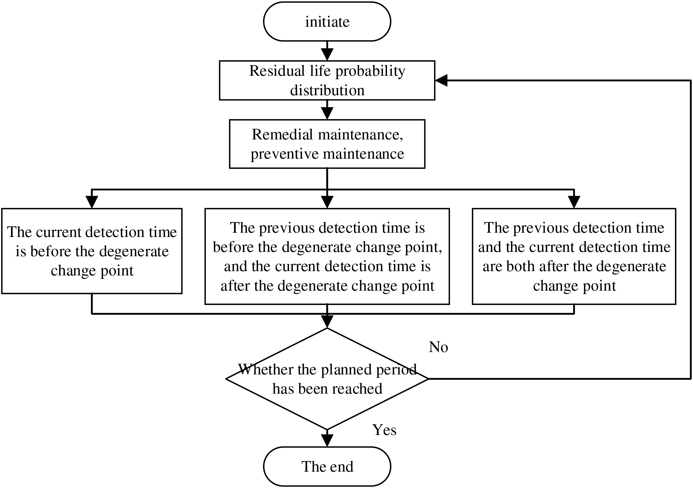
Figure 2: Maintenance policy flowchart

4  Example Analysis

To demonstrate the viability of the proposed method, an exemplary study is conducted using a case from Reference [24]. Initially, the data is processed according to the case study, resulting in the output power degradation data shown in Fig. 3, which represents 12 years (1200 cycles) of service for S73L47.

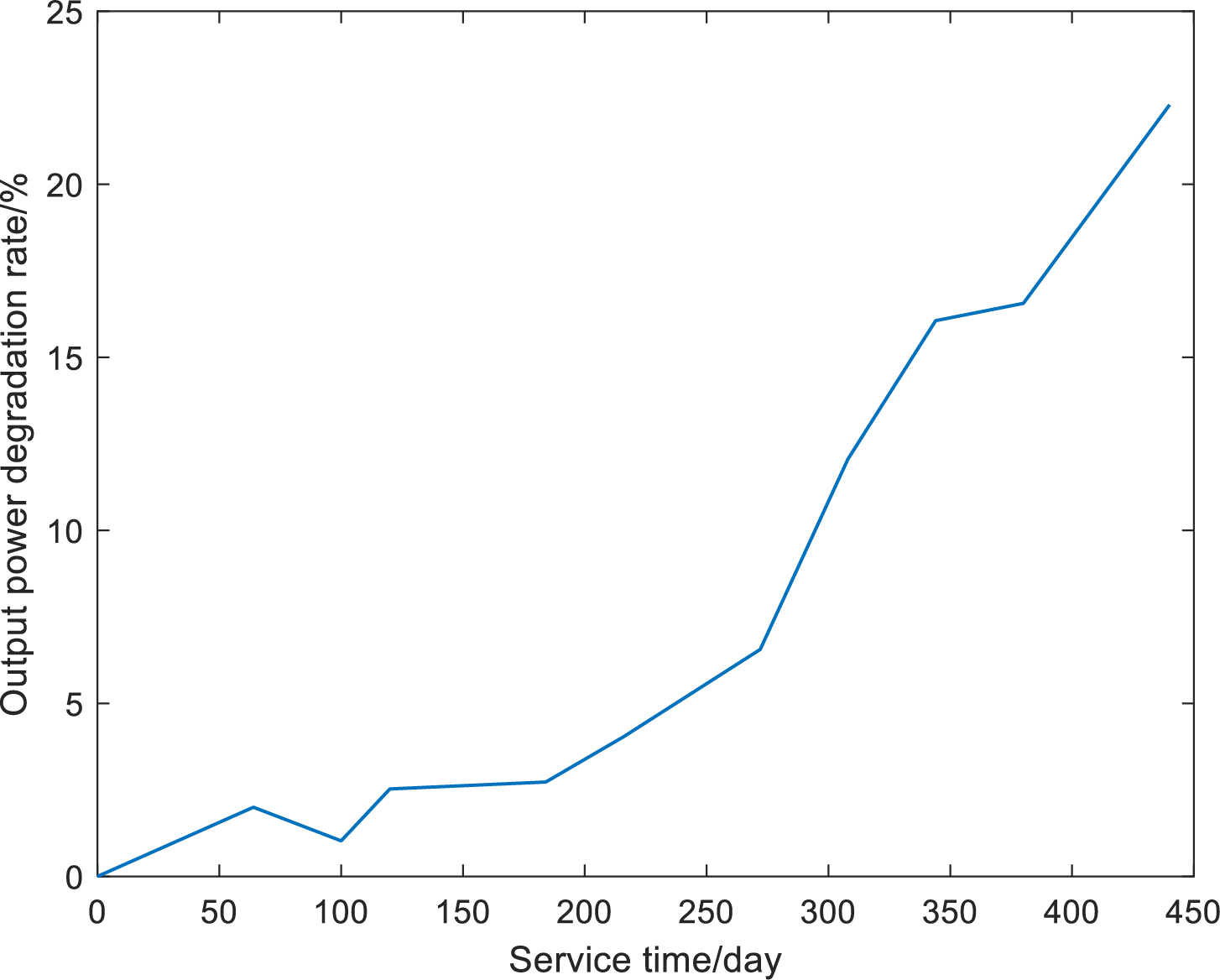
Figure 3: Degradation curve

The S73L47 power decay model stipulates that the actual output power of the PV module decreases to 80% of its initial output power P0, which is established as its scrap threshold [25]. Initially, Schwarz information criterion (SIC) is employed to monitor the change point of the degradation model. Fig. 4 illustrates the corresponding trend of SIC value changes, which reveals three distinct minimum peaks. The peak at the 152nd monitoring point is attributed to early equipment break-in and production issues, while the peak at the 970th monitoring point may result from equipment aging in the later stages, leading to a change point. As this study utilizes a two-stage random degradation modeling approach, the maximum peak τ=671 is identified as the change point in the PV module’s degradation process.

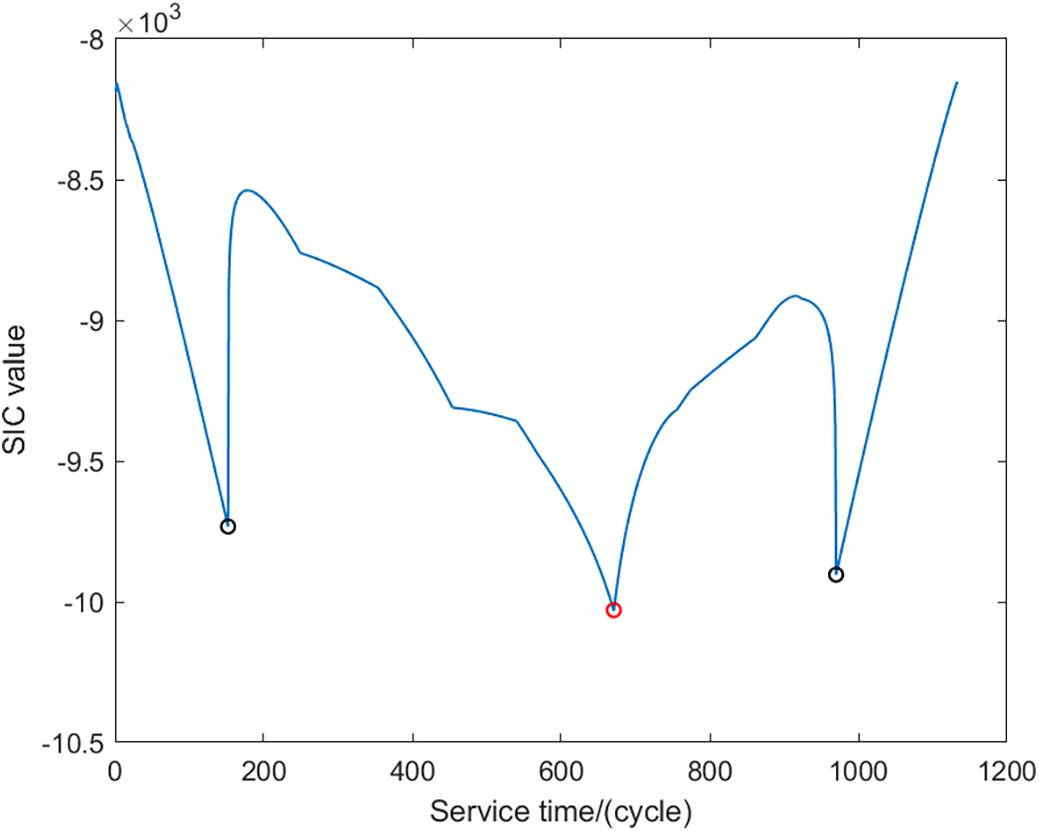
Figure 4: SIC value of the PV module

Reference [26] observes a two-stage phenomenon in PV modules through blackout experiments, aligning with the stage division hypothesis of the Wiener degradation model presented in this paper. Furthermore, as suggested by [22], a comparison of the average degradation curves for the four groups of PV modules is made in Fig. 5, where the degradation curve of the S73L47 PV module closely adheres to the two-stage process. Additionally, Fig. 5 reveals that the proposed method exhibits smaller errors compared to linear and nonlinear methods, further supporting its efficacy.

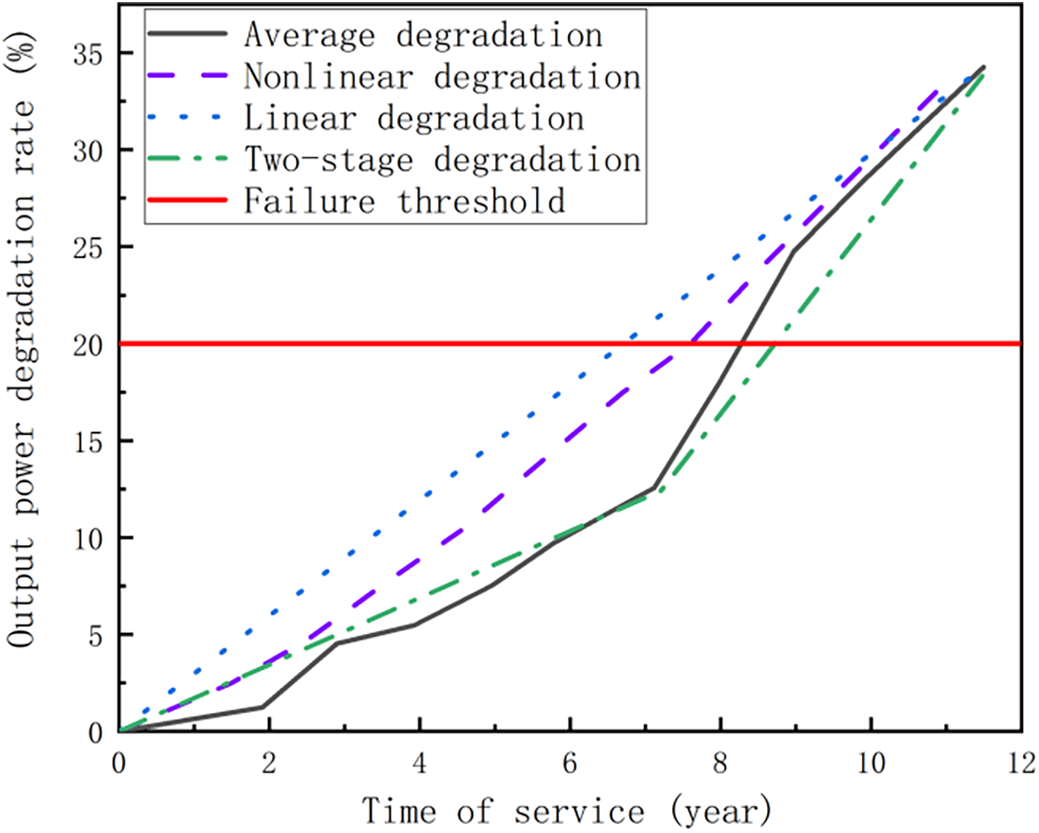
Figure 5: Comparison of component performance degradation trajectories

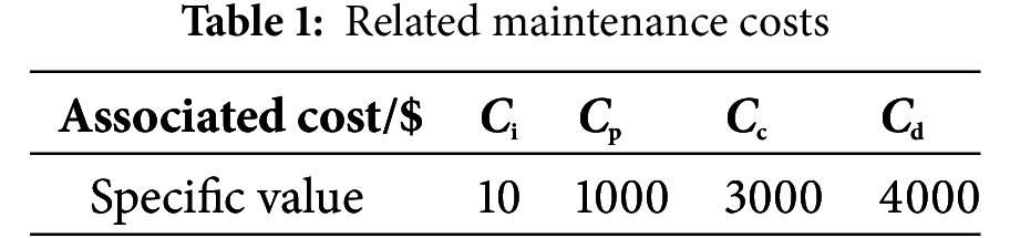
Table 1 presents the costs associated with the predictive maintenance strategy for the PV module and corresponding parameter settings.

To evaluate the effectiveness of the proposed predictive maintenance strategy, we compare it with established methodologies.

Strategy A (Reactive Corrective Maintenance)

The maintenance strategy employed is failure-triggered, wherein no continuous real-time condition monitoring occurs during the PV module’s operational lifespan. Maintenance procedures are initiated only when the power output degradation surpasses a predetermined safety threshold. This approach is particularly appropriate for scenarios characterized by well-defined degradation trajectories and manageable failure consequences.

Strategy B (Static Periodic Maintenance Based on Wiener Process)

A fixed-interval maintenance system is implemented, wherein periodic comprehensive maintenance is scheduled according to the device’s nominal service life. Each maintenance intervention restores the degradation state to its initial level, without considering the historical maintenance effects on actual operational conditions.

Strategy C (CBM Based on Two-Stage Wiener Process)

This strategy is an advanced operations and maintenance (O&M) solution integrating two-phase degradation characteristics. Through continuous performance data monitoring, a dual-mode degradation recognition model is developed to facilitate dynamic maintenance timing decisions and optimize resource allocation.

Under the aforementioned three scenario types, the optimized maintenance strategy results for the PV module are as follows:

Strategy A (Reactive Corrective Maintenance)

Analysis of implementation data indicates that this strategy initiates a single technical intervention after 11.2 years (4088 days) of system operation, coinciding with the PV unit’s output power degradation to 80% of its rated capacity. The economic assessment shows that this approach incurs a daily maintenance cost of ¥11.71 RMB, with total lifecycle operational expenditures amounting to ¥47,800 RMB, rendering it appropriate for application scenarios with low risk tolerance.

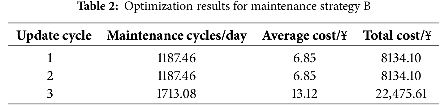
Strategy B (Static Periodic Maintenance Based on Wiener Process)

As demonstrated in Table 2, the adoption of a fixed 3.25-year (1187.46-day) maintenance interval resulted in performance threshold failures occurring before the third maintenance cycle, necessitating emergency repairs through passive response mechanisms. This operational approach leads to an increase in total maintenance costs to ¥38,743.81 RMB, representing an 8.3% cost premium compared to the baseline solution.

Strategy C (CBM Strategy Based on Two-Stage Wiener Process)

The CBM strategy is implemented using a fixed 1469.58-day cycle. Based on the data presented in Table 3, this approach results in a final average total maintenance cost of ¥32,821.4 RMB. This represents cost reductions of 31.4% and 15.3% compared to Strategies A and B, respectively, demonstrating substantial maintenance cost savings. The optimization process for Strategy C is illustrated in Fig. 6.

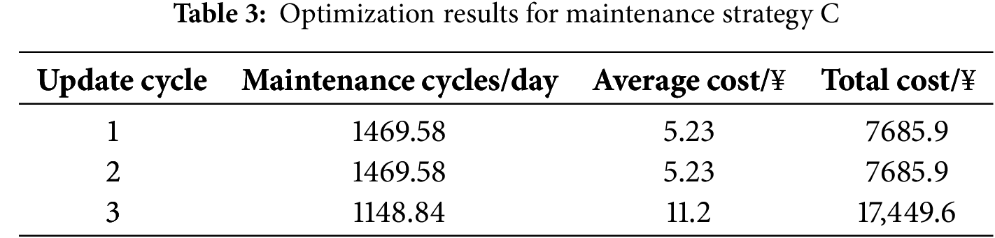
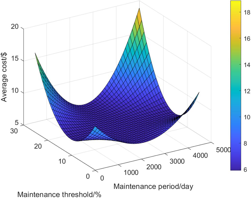
Figure 6: Maintenance thresholds and monitoring intervals vs. average costs

To assess the effects of maintenance thresholds and intervals on the average maintenance cost of PV module maintenance strategies, sensitivity analysis is conducted using varying values. Figs. 7 and 8 illustrate the average maintenance costs under different maintenance thresholds and intervals, respectively.

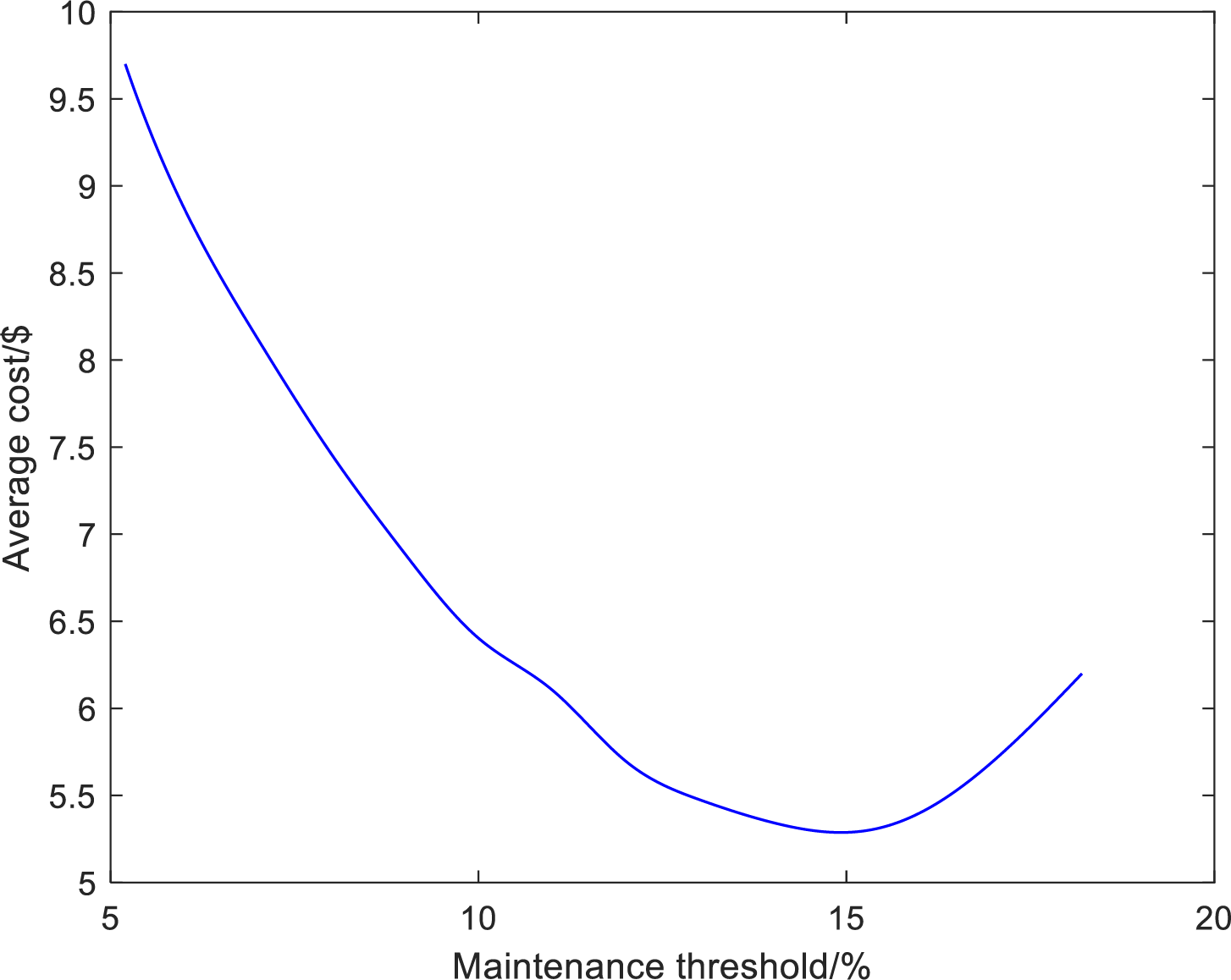
Figure 7: Average maintenance cost for different maintenance thresholds

Figure 8: Average maintenance cost at different maintenance intervals

The maintenance threshold denotes the quantified critical standard that initiates a PV module maintenance intervention, typically based on a power decay threshold. For instance, this threshold may be reached when the module’s output power decreases to 80% of its initial value. A higher maintenance threshold indicates a more lenient definition of PV module degradation failure, resulting in reduced average maintenance costs. Conversely, a lower maintenance threshold implies a more stringent definition of degradation failure, leading to increased average maintenance expenses. As illustrated in Fig. 7, the optimal maintenance threshold for the initial maintenance update cycle occurs when the PV module’s output power degradation reaches 14.88% of its initial power. At this point, the average maintenance cost of the module is minimized.

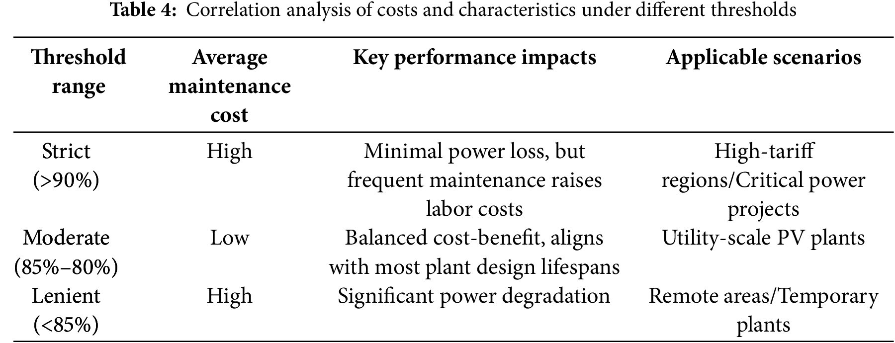
Through the classification of various threshold ranges, this study examines their effects on maintenance expenses and overall system efficiency, as illustrated in Table 4.

The average maintenance cost of the PV system exhibits a U-shaped relationship with the maintenance interval, with its lowest point determined by a multi-parameter dynamic balance. In the short interval area (left branch), high-frequency maintenance results in increased labor and spare parts costs. The optimal interval (lowest point) represents the balance between preventive maintenance and the risk of failure. As illustrated in Fig. 8, the optimal maintenance period for the first maintenance update cycle is 1475.78 days, at which point the average maintenance cost of the module is minimized. In the long interval area (right branch), the failure rate increases significantly, and power generation loss costs become predominant. Furthermore, the timing analysis of the two-stage degradation model indicates that the first periodic monitoring is appropriate after the performance turning point. This pattern aligns with the reliability bathtub curve theory: in the first stage (early stable period), the system failure risk is low and primarily affected by accidental factors. Upon entering the second stage (wear and degradation stage), material aging leads to continuous deterioration of performance indicators, and the failure risk escalates rapidly with extended operating time. At this juncture, it becomes necessary to mitigate the probability of sudden failure through increased monitoring frequency.

5  Conclusions

This paper proposes a visual maintenance method for PV modules based on a two-stage Wiener degradation model. This approach introduces a two-stage residual life prediction method for PV modules, which, compared to periodic maintenance, avoids unnecessary maintenance work when there is no actual failure or performance degradation. The method incorporates a penalty cost for delayed fault detection, aligning more closely with the actual maintenance status of PV modules and effectively improving the development of an optimal O&M cycle strategy. The visual maintenance strategy adopts long-term average cost rate minimization as its optimization objective, considering comprehensive costs to enhance resource utilization efficiency. This approach provides robust data support for optimizing maintenance strategies. Comparative analysis with ex-post corrective maintenance schemes demonstrates that this visual maintenance approach, based on the remaining life of the two-stage degradation process, reduces average maintenance costs while increasing the service life and operational benefits of PV modules.

Acknowledgement: Not applicable.

Funding Statement: This research was supported by the National Natural Science Foundation of China (51767017), the Basic Research Innovation Group Project of Gansu Province (18JR3RA133), and the Industrial Support and Guidance Project of Universities in Gansu Province (2022CYZC-22).

Author Contributions: The authors confirm their contributions to the paper as follows. Study conception and design: Jie Lin; data collection: Hongchi Shen; analysis and interpretation of results: Tingting Pei; draft manuscript preparation: Yan Wu. All authors reviewed the results and approved the final version of the manuscript.

Availability of Data and Materials: The data supporting this study are included within the article.

Ethics Approval: Not applicable.

Conflicts of Interest: The authors declare no conflicts of interest to report regarding the present study.

Nomenclature

References

1. Osmani K, Haddad A, Lemenand T, Castanier B, Ramadan M. A review on maintenance strategies for PV systems. Sci Total Environ. 2020;746:141753. doi:10.1016/j.scitotenv.2020.141753. [Google Scholar] [PubMed] [CrossRef]

2. Fievez M, Singh Rana PJ, Koh TM, Manceau M, Lew JH, Jamaludin NF, et al. Slot-die coated methylammonium-free perovskite solar cells with 18% efficiency. Sol Energy Mater Sol Cells. 2021;230:111189. doi:10.1016/j.solmat.2021.111189. [Google Scholar] [CrossRef]

3. Zhang Z, Li H, Li T, Zhang J, Si X. An optimal condition-based maintenance policy for nonlinear stochastic degrading systems. Reliab Eng Syst Saf. 2024;251:110349. doi:10.1016/j.ress.2024.110349. [Google Scholar] [CrossRef]

4. Baldus-Jeursen C, Côté A, Deer T, Poissant Y. Analysis of photovoltaic module performance and life cycle degradation for a 23 year-old array in Quebec. Canada Renew Energy. 2021;174:547–56. doi:10.1016/j.renene.2021.04.013. [Google Scholar] [CrossRef]

5. Abdulla H, Sleptchenko A, Nayfeh A. Photovoltaic systems operation and maintenance: a review and future directions. Renew Sustain Energy Rev. 2024;195:114342. doi:10.1016/j.rser.2024.114342. [Google Scholar] [CrossRef]

6. Abubakar A, Almeida CFM, Gemignani M. Solar photovoltaic system maintenance strategies: a review. Polytechnica. 2023;6(1):3. doi:10.1007/s41050-023-00044-w. [Google Scholar] [CrossRef]

7. Perdue M, Gottschalg R. Energy yields of small grid connected photovoltaic system: effects of component reliability and maintenance. IET Renew Power Gener. 2015;9(5):432–7. doi:10.1049/iet-rpg.2014.0389. [Google Scholar] [CrossRef]

8. Baklouti A, Mifdal L, Dellagi S, Chelbi A. An optimal preventive maintenance policy for a solar photovoltaic system. Sustainability. 2020;12(10):4266. doi:10.3390/su12104266. [Google Scholar] [CrossRef]

9. Yin D, Mei F, Zheng J, He W, Qi X. Determination method of optimal operation and maintenance cycles for distributed photovoltaic system. 2022;42(5):135–41. doi:10.16081/j.epae.202202020. [Google Scholar] [CrossRef]

10. Goyal D, Pabla BS. Condition based maintenance of machine tools—a review. CIRP J Manuf Sci Technol. 2015;10:24–35. doi:10.1016/j.cirpj.2015.05.004. [Google Scholar] [CrossRef]

11. Chen W, Li M, Pei T, Sun C. Research on opportunity maintenance strategy for PV power generation systems considering random impact. Electr Eng. 2024;106(6):7819–30. doi:10.1007/s00202-024-02470-0. [Google Scholar] [CrossRef]

12. Chen W, Sun C, Pei T, Li M, Lei H. Opportunistic maintenance strategies for PV power systems considering the structural correlation. Electr Eng. 2024;106(4):3947–59. doi:10.1007/s00202-023-02182-x. [Google Scholar] [CrossRef]

13. Li X, Ran Y, Wan F, Yu H, Zhang G, He Y. Condition-based maintenance strategy optimization of meta-action unit considering imperfect preventive maintenance based on Wiener process. Flex Serv Manuf J. 2022;34(1):204–33. doi:10.1007/s10696-021-09407-w. [Google Scholar] [CrossRef]

14. Wang Y, Li X, Chen J, Liu Y. A condition-based maintenance policy for multi-component systems subject to stochastic and economic dependencies. Reliab Eng Syst Saf. 2022;219:108174. doi:10.1016/j.ress.2021.108174. [Google Scholar] [CrossRef]

15. Luo Y, Zhao X, Liu B, He S. Condition-based maintenance policy for systems under dynamic environment. Reliab Eng Syst Saf. 2024;246:110072. doi:10.1016/j.ress.2024.110072. [Google Scholar] [CrossRef]

16. Lei H. Research on residual life prediction and maintenance strategy of photovoltaic power generation system based on Wiener process [M.S. thesis]. Lanzhou, China: Lanzhou University of Technology; 2023. [Google Scholar]

17. Wang H, Zhao Y, Ma X. Remaining useful life prediction using a novel two-stage Wiener process with stage correlation. IEEE Access. 2018;6:65227–38. doi:10.1109/ACCESS.2018.2877630. [Google Scholar] [CrossRef]

18. Zhang A, Wang ZH, Zhao ZP, Qin XG, Wu QR, Liu CR. Two-phase nonlinear Wiener process for degradation modeling and reliability analysis. Syst Eng Electr. 2020;42(4):954–9. (In Chinese). [Google Scholar]

19. Chen K, Liu J, Guo W, Wang X. A two-stage approach based on Bayesian deep learning for predicting remaining useful life of rolling element bearings. Comput Electr Eng. 2023;109:108745. doi:10.1016/j.compeleceng.2023.108745. [Google Scholar] [CrossRef]

20. Guan Q, Wei X, Bai W, Jia L. Two-stage degradation modeling for remaining useful life prediction based on the Wiener process with measurement errors. Quality Reliab Eng. 2022;38(7):3485–512. doi:10.1002/qre.3147. [Google Scholar] [CrossRef]

21. Zhang P, Hu CH, Bai C, Zhang Y, Zhang JX. Remaining useful life estimation method for two-phase degradation system with random effects. China Testing. 2019 Jan;45(1):1–7. (In Chinese). [Google Scholar]

22. Shen H, Pei T, Wu Y, Lin J. Remaining life prediction method for photovoltaic modules based on two-stage Wiener process. Energy Eng. 2025;122(1):331–47. doi:10.32604/ee.2024.055611. [Google Scholar] [CrossRef]

23. Yao YQ. Research on reliability modeling and condition-based maintenance strategy of two-phase degradation system [M.S. thesis]. Tianjin, China: Tianjin University; 2020. [Google Scholar]

24. Liu WD, Wen G, Yan W, Luo J, Jiang XH. Field lifetime assessment of photovoltaic modules based on degradation data-driven and nonlinear Gamma processes. Comput Integr Manuf Syst. Dec. 2021;27(12):3494–502. (In Chinese). [Google Scholar]

25. Jordan DC, Kurtz SR, VanSant K, Newmiller J. Compendium of photovoltaic degradation rates. Progress Photovolt. 2016;24(7):978–89. doi:10.1002/pip.2744. [Google Scholar] [CrossRef]

26. Pradhan S, Kundu S, Bhattacharjee A, Mondal S, Chakrabarti P, Maity S. Thermal and optical analysis of industrial photovoltaic modules under partial shading in diverse environmental conditions. Sol Energy. 2024;284:113097. doi:10.1016/j.solener.2024.113097. [Google Scholar] [CrossRef]