Research on Flexible Load Aggregation and Coordinated Control Methods Considering Dynamic Demand Response

1  Introduction

With the accelerated progress of the construction of new power systems [1], the modern power system is gradually evolving towards source-load interaction and large-scale consumption of new energy. It exhibits characteristics such as increasingly abundant power resources on the source side and flexible and variable load demands of end-users. On one hand, the large-scale integration of new energy into the grid leads to obvious spatial and temporal imbalances in power balance. The pressure of peak-frequency regulation is prominent, and the continuous increase in peak electricity load also poses challenges to the regulation capacity of the power system. The existing power generation-tracking-load mode can no longer adapt to the development of the power grid. On the other hand, load-side equipment has become more diversified. Due to their characteristics of large quantity, fast response, and flexible control, large-scale adjustable flexible loads have gradually become important regulating resources in scenarios such as peak-shaving and valley-filling, smoothing new energy fluctuations, and providing auxiliary services [2].

As an effective means to address the problems of large-scale distributed energy access and optimized operation, the distribution network urgently needs to tap the potential of flexible regulation of user-side flexible resources. This not only promotes the optimal allocation of resources, improves the reliability of the system and power quality but also enhances the system’s acceptance capacity for renewable energy. However, in terms of demand-side resources, load-side equipment is more diverse [3]. For example, flexible resources such as air conditioners, electric vehicles, and distributed energy storage not only have the advantages of large scale, fast response, and high flexibility but also are not conducive to directly participating in power regulation and control due to their small individual capacity, large number, and high randomness. Currently, research on massive and multi-type flexible loads still suffers from the lack of common modeling methods and large errors in coordination and control. There is still a lack of systematic research on the modes and models for multi-type flexible resources to participate in peaking optimization, making it difficult to meet the requirements of the rapid development of distribution networks.

Therefore, taking multiple types of flexible loads on the user side of the distribution network as the research object, conducting research on its general aggregation modeling method and coordination and control method, solving the unified modeling problem of multiple types of flexible loads, and studying the refined coordination and control strategy from the perspective of flexible load regulation and control, and guiding the large-scale flexible loads on the demand side to deeply participate in the operation of the distribution network have become the main challenges faced by modern distribution networks. In addition, conducting the above-mentioned research is of great significance. It can not only effectively improve the coordination and control ability of active distribution networks with the participation of flexible loads but also provide support for peak voltage and frequency regulation of distribution networks and smoothing new energy fluctuations.

2  Literature Review

With the growing integration of renewable energy sources in recent years, the power grid has undergone a profound transformation. Although this integration holds great promise for a sustainable future, it has given rise to a series of challenges. The intermittent nature of renewable power generation is a prime concern. For instance, solar power output is directly contingent on sunlight availability, which fluctuates with weather conditions and time of day. Similarly, wind power generation is highly dependent on wind speed and direction. Such intermittency can trigger substantial fluctuations in grid frequency and voltage, thereby jeopardising the stable operation of the power grid [4].

Demand response (DR) has emerged as a pivotal solution to overcome these challenges. Initially, basic DR programs predominantly focused on directly managing large industrial loads to curtail the peak loads. However, with the continuous advancement of smart grid technology and the growing penetration of distributed energy resources, DR has evolved into a far more complex and multifaceted paradigm [5]. Flexible loads and demand responses play an indispensable role in contemporary grids. Flexible loads, encompassing thermostatically controlled loads, electric vehicles, and distributed energy storage, can alter power flow. This characteristic not only complicates the fault current and voltage during grid faults but also leads to changes in the electrical parameters when the demand response is implemented. Existing research faces difficulties in accurately modelling their behaviour during faults and effectively incorporating them into fault-location algorithms [6]. Yang et al. emphasized that as the power grid evolves, there is an ongoing need for novel methods and technologies to ensure its stable operation, and the fault current-constrained impedance-based method offers valuable insights in this area [7]. The evolution of DR has spurred extensive research on diverse response and control methods. Among these, flexible-load aggregation has garnered significant attention. Flexible loads can adjust their power consumption or generation in response to grid signals. This capacity can effectively enhance grid flexibility and its ability to integrate renewable energy, thereby contributing to the overall stability and reliability of the power system [8]. In addition, flexible load aggregation modelling builds a physical model based on the working principle of a flexible load. Subsequently, methods such as the superposition method [9], Monte Carlo simulation method [10], state sequence model [11], and mixed logic model [12] are used to build the adjustable power calculation model of the load group.

2.1 Modeling of Flexible Load Aggregation

2.1.1 Thermostatic Control of Loads

A thermoelectric equivalent parameter model is commonly employed for thermostatically controlled loads. This model induces power variations by modifying the temperature set points using the equivalent thermal resistance and thermal capacitance as the foundation for clustering and grouping. Subsequently, techniques such as Monte Carlo sampling, state transitions, and state queues were utilised to analyse the operating states of the load clusters. This analysis yields either the aggregated power of the load clusters or the probability distribution of the load cluster state variables over time. Finally, the total aggregated power of the load clusters was determined by applying the appropriate weights to all load clusters.

In [13], an air-conditioning load aggregation response potential assessment and control strategy that considers multiple factors was proposed. This strategy comprehensively considers aspects such as the users’ thermal comfort, willingness, and controllability to ascertain the aggregation response potential. A joint scheduling model was then developed by integrating the response characteristics of basic flexible loads. This model enables precise control of the control layer and mitigates the adverse impacts triggered by power dips. In [14], a time-frequency domain model was constructed using an inverter air conditioner as a representative temperature-controlled load to evaluate the potential of temperature-controlled loads to provide frequency-regulation services. Through simulation, the significance of temperature-controlled load participation in frequency regulation for the power system’s frequency stability was analysed, and a hybrid control method that considers users’ electricity-use comfort levels was proposed, which plays a role in regulating the power system’s frequency. In [15], a real-time scheduling model and an improved proportional aggregation method for distribution networks were proposed. This simplifies complex problems based on linearised power flow with power loss sensitivity. Distributed, thermostatically controlled loads are aggregated for power regulation as a whole to offset power imbalances caused by the uncertainty of intermittent renewable energy output. Simulation results demonstrate that the proposed method accurately aggregates distributed thermostatically controlled loads and reduces unbalanced power even when user model parameters are heterogeneous. In [16], a thermostatic load hierarchical scheduling strategy is presented. At the aggregator layer, an arriving-law-law-based sliding mode controller is designed to manage heterogeneous thermostatic load aggregators, and a genetic algorithm is applied to solve the optimization problem at the agent layer. Simulation results indicate that the strategy considers consumer discomfort, the potential capacity of multiple aggregators, and the optimal allocation of frequency regulation signals to each load aggregator, achieving both economic cost optimization and consumer comfort improvement.

2.1.2 Electric Vehicles

Electric vehicles have become a vital component of flexible loads in the power grid. As the number of electric vehicles connected to the grid continues to grow exponentially, their impact on the power system cannot be overlooked. In addition to prior research, new studies have emerged. For example, in [17], a novel charging and discharging optimization strategy for electric vehicles in a multi-user scenario is proposed. This strategy considers the travel patterns of different users and real-time grid conditions to optimize the charging and discharging behaviour of electric vehicles, with the aim of reducing the grid load’s peak-valley difference. Zhang et al. [18] explore the impact of vehicle-to-grid (V2G) technology on the power system’s frequency regulation. The results show that V2G can effectively provide frequency regulation services and enhance the power system’s stability.

Electric vehicles are typically integrated by consolidating dispersed electric vehicle load resources within a specific region. Leveraging their charging and discharging flexibility, they participate in grid demand response and scheduling to optimize load allocation. This not only effectively mitigates the fluctuations of renewable energy but also reduces system operating costs, thereby enhancing the stability and reliability of the power grid. In literature [19], a load combination optimization control method that takes into account electric vehicles and temperature-controlled load clusters is proposed. A three-stage rebound load model is established by aggregating single electric vehicles and temperature-controlled load clusters to optimize the composition of user groups participating in peak staggering and avoidance and the amount of load regulation, thus enabling favourable interaction between distributed load resources and the power grid in terms of supply and demand. In [20], an EV aggregation model that considers the flexibility of charging and discharging modes is established. This model fully accounts for the flexibility of EV charging and discharging modes, clusters EVs based on their characteristic parameters, and assigns corresponding charging and discharging modes to expand the feasible region of EV energy and power and tap into more adjustable capacity. Simulation results validate the effectiveness of the aggregation model in enhancing the adjustable capacity of EVs, which helps address the security and stability issues caused by the disorderly connection of large-scale EVs to the power grid. In [21], a decomposable aggregated region approach, comprising an inner approximate feasible region and an equivalent system cost function, is developed for electric vehicles to fully exploit their potential flexibility. First, EV loads are modelled through an operating region that considers demand and EV parameters. Second, the inner approximation region is formulated to obtain the maximum potential flexibility of EVs by transforming the basic homotopy polyhedron. Finally, the aggregated model participates in economic dispatch. Simulation tests demonstrate the great potential of this approach for economic dispatch prior to the system day and ensure the feasibility of the solution. In [22], fully considering the substantial impact of the large-scale development of electric vehicles on the power grid and the differences in the characteristics of different types of electric vehicles, an electric vehicle load aggregation method based on the clustering of SOM neural networks is proposed. Different types of electric vehicles are clustered, and the clustering results are analyzed to further improve the accuracy of the aggregation model. Moreover, reference [23] proposed a self-anti-disturbance control (ADRC) method for stabilizing electric vehicle (EV) systems without the need for model identification. This method can effectively handle the uncertainties in the EV system and enhance its stability, offering a new perspective for the control of electric vehicle systems in the power grid, especially when considering the intricate interaction between electric vehicles and the grid.

2.1.3 Distributed Energy Storage

Distributed energy storage involves dynamically modelling and aggregating the characteristics of multiple distributed storage units, such as power throughput capacity, state of charge, and capacity, to optimize the configuration and flexible scheduling of storage resources. This model employs adaptive balancing technology to simulate the dynamic regulation capabilities of individual storage units. Parameters such as power regulation degree, adaptive balancing degree, and capacity contribution are used to assess the potential for storage aggregation, thereby enhancing the response capabilities and overall efficiency of storage resources in grid applications such as peak shaving and frequency regulation.

In [24], a distributed energy storage aggregation method based on SOC balancing is proposed to meet the requirements of power system dispatch operation. Distributed energy storage within the scheduling partition is aggregated into large-scale cluster storage with stable parameters, and the parameters required for the scheduling optimization model are characterized. The power sequences of typical scenarios are used to test the clustering regulation capability after energy storage clustering. Validation based on power data from the HRP38 system is carried out to verify the correctness and effectiveness of the proposed clustering method. In [25], large-scale distributed energy storage is aggregated into a small number of feature clusters based on the K-means++ algorithm by combining typical feature quantities, and an aggregation scheduling model is established to reduce the peak-to-valley difference of loads faced by the distribution network and to address the issue of large-scale distributed energy storage resources participating in distribution network operation. Simulation verifies that the proposed method can conduct reasonable scheduling of distributed energy storage and enhance the feasibility of optimization. In [26], to boost the fluctuation-accommodating capacity of renewable energy generation, improve the load profile, and enhance operational security and economics, a unit commitment-based multi-objective optimization problem is proposed for optimizing the aggregation and control of multiple types of energy storage systems. This problem respects operational security constraints, with power system operational economics and the utilization efficiency of the energy storage system as optimization objectives. Finally, the proposed optimal aggregation and control method is demonstrated using a modified IEEE 33-bus power distribution system, and the Pareto frontier and compromise optimal solutions of the multi-objective optimization problem are obtained.

2.2 Optimal Scheduling of Flexible Loads

In the area of optimal scheduling of flexible loads, new energy consumption, peaking, frequency regulation, and other operational scenarios are typically considered. Depending on the specific demands of these scenarios, the minimum grid operation cost, the minimum load scheduling deviation, or the maximum profit of the aggregator are respectively adopted as the objective function for optimal scheduling.

In [27], a heterogeneous load aggregation control method based on the controllable margin of the flexible load is proposed by establishing a generalized energy storage aggregation model. This method not only achieves system peak shaving and valley filling but also reduces the system operation cost. In [28], an integrated energy system model is proposed based on the concept of an energy hub that combines wind energy storage, gas turbines, and flexible loads. This model fully exploits the panning, shifting, and curtailment characteristics of demand-side flexible loads formulates a dispatch model with the objective of cost minimization, and solves it using a particle swarm optimization algorithm to rationally dispatch flexible loads to reduce peaks and valleys and lower the system cost. The results show that the participation of flexible load scheduling can effectively improve the stability and comprehensive efficiency of the system. In [29], based on the residential electricity consumption differentiation in load regulation and considering the comprehensive satisfaction degree of typical residential electricity equipment, an analysis model of residential flexible load adjustable potential is constructed. This model can effectively support the optimal bidding decision-making of load aggregator enterprises and provides a reference for the optimal regulation of load aggregator resources. In [30], a method for predicting the demand response potential of user clusters based on the user’s historical load, temperature, and tariff data is proposed. This method calculates the eigenvalues of each user’s electricity consumption behaviour, forms an indicator system for assessing the type of user, and finally validates the effectiveness of the proposed method through comparative analysis with actual electricity regulation data. Yan et al. [31] have modelled the complex and uncertain dynamic characteristics in various components of the multi-area interconnected power system. This research provides crucial insights into the overall operation and control of the power system, especially when considering the integration of renewable energy and demand response, which is closely related to the research on flexible loads in this paper.

2.3 Research Motivation

The power grid’s progression towards greater integration of renewable energy has led to an augmented reliance on demand response. As DR has evolved from the simplistic peak-load reduction via large-industrial-load control to a more intricate system involving diverse flexible loads, the imperative for effective flexible load management has become more pronounced. The various types of flexible loads, including thermostatically controlled loads, electric vehicles, and distributed energy storage, each exhibit distinct physical models and operating characteristics.

Current research has achieved certain advancements in the coordinated control of flexible loads, particularly for air-conditioning and electric-vehicle loads. Nevertheless, the majority of existing studies concentrate on the aggregation control of a single type of load. Owing to the significant disparities in physical models and operating characteristics among different types of flexible loads, there is a dearth of a universal and unified approach for aggregating multiple types of flexible load resources. In real-world operational scenarios, the structural heterogeneity among multiple types of loads exerts a crucial influence on the formulation of joint control methods for load clusters. Furthermore, there is a lack of in-depth and systematic research on the coordinated participation of multi-variable heterogeneous flexible loads in dynamic demand response and sequential control. The aggregation modelling and coordinated control strategies for flexible loads are often disjointed.

Consequently, the development of a universal and unified aggregation model for heterogeneous flexible load resources to achieve coordinated control is an urgent problem in current research. This paper endeavours to bridge this gap by proposing a multivariate, heterogeneous, flexible load aggregation and coordinated control method oriented towards dynamic demand response. By establishing a time-domain aggregation model of multivariate heterogeneous flexible loads, constructing a refined prediction method, and using a parallel Markov chain model to evaluate switch state transfer probability, this method can effectively realize dynamic demand response within the framework of intra-day scheduling plans, thereby enhancing the stability and efficiency of the power grid.

3  Multivariate Heterogeneous Flexible Loads and Coordinated Control Framework

3.1 Classification of Flexible Loads

Flexible loads refer to the loads whose electricity consumption can be adjusted according to the received instructions within the range specified by the user or transferred from one time period to another while keeping the total electricity consumption unchanged [32]. Compared with rigid loads, whose electricity consumption behavior is relatively constant and whose power size cannot be adjusted, flexible loads have the characteristics of virtual energy storage and flexible scheduling. On the one hand, they make up for the insufficient regulation ability of the power generation side, and on the other hand, they cut peaks and fill valleys and optimize the allocation of electricity resources.

According to different scheduling methods, flexible loads can be divided into reducible loads, transferable loads and shiftable loads [33], as shown in Fig. 1.

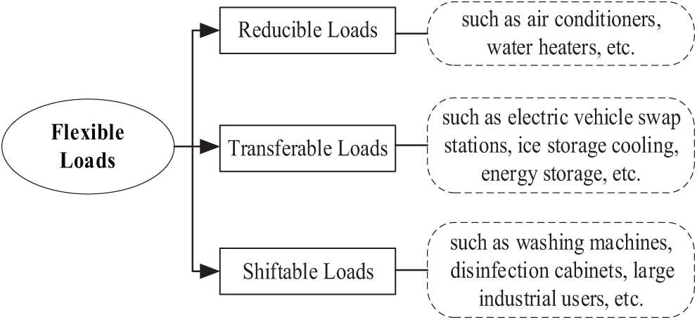
Figure 1: Typical types of flexible loads

In the realm of power systems, different types of loads play crucial roles in power management and grid operation. Reducible loads, such as air conditioners and water heaters, can be decreased to a certain degree in response to demand. Transferable loads, like electric vehicle swap stations, ice storage cooling, and energy storage, maintain the same total electricity consumption within a scheduling cycle but allow for flexible adjustment of consumption in each time period. Shiftable loads, including washing machines, disinfection cabinets, and large industrial users, have a fixed electricity consumption duration and are non-interruptible, with only their electricity consumption curves being shiftable as a whole across different time periods.

From the perspective of energy conversion, the above classification method of flexible loads focuses more on the adjustable characteristics of the loads but does not consider factors such as equipment difference characteristics, heat and cold conversion, and the size of regulation ability. There are also great difficulties in coordinated control, which is difficult to meet different power demand scenarios and needs to be aggregated to achieve hierarchical control.

3.2 Hierarchical Coordinated Control Architecture of Flexible Loads

Flexible loads are widely distributed, have small capacity and low voltage levels, and mostly appear in the form of distributed scheduling units. They can participate in active distribution networks or microgrids independently, or be aggregated to form clusters to participate in the regulation of the main network together [34]. Among them, the hierarchically coordinated control architecture of flexible loads with aggregators as the core is shown in Fig. 2.

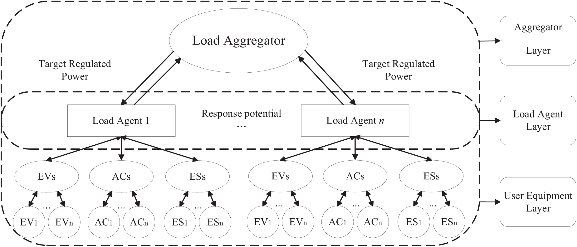
Figure 2: Hierarchical coordinated control architecture of flexible load aggregator

In a load management system, the load aggregator at the aggregator layer plays a crucial role. It analyzes the flexible load resources within its purview, computes the maximum response potential range of diverse aggregated flexible load clusters, and feeds this information back to the dispatching center to receive the issued adjustable target power. Post evaluation and calculation, it initially distributes the power and passes it on to the load agents for separate management, all the while leveraging the two-way communication mechanism to enhance coordinated control. At the load agent layer, each load agent obtains the target power adjustment amount from the upper-level aggregator. Within the real-time time scale, it monitors load changes in the load cluster and continuously updates parameters such as load status and response potential. Based on the control target and the updated response potential, it conducts the secondary distribution of the target power among the load clusters and then controls the user equipment. At the user equipment layer, different types of user equipment gather load parameters and operating status information via smart sockets or smart switches and upload parameters like load transfer status and controllable margin to the load agent through user-side edge computing. In accordance with the control indicators allocated and issued by the load agent, it dynamically controls the sequence, directly calling the load to fulfill the demand-side response target.

4  Mathematical Modeling for Flexible Load Aggregation

4.1 Individual Mathematical Model of Flexible Loads

The flexible load cluster has the typical characteristics of “multivariate heterogeneity,” and the physical modeling methods of different loads are also different [35]. Fully considering the characteristics of typical temperature-controlled loads (TC), electric vehicles (EV) and energy storage devices (ES), the flexible load individual modeling is carried out through the generalized model.

4.1.1 Temperature-Controlled Loads

For temperature-controlled loads such as air conditioners and water heaters, the parameters are heterogeneous but the working logic tends to be unified, which is suitable for the following equivalent thermodynamic state evolution model:

Tint+1=Tot+1+RQTCt−(Tot+1+RQTCt−Tint)e−ΔtRC(1)

where Tint is the internal temperature of the temperature control device at time t, Tot+1 is the external ambient temperature at time t + 1, QTCt is the equivalent thermodynamic power of the temperature control device at time t, R is the equivalent thermal resistance, C is the equivalent heat capacity, and Δt is the time scale.

Considering the electrical heating (cooling) energy conversion efficiency of the temperature control equipment, which is λ.

QTCt=λPTCt(2)

Then, the above formula can be transformed into:

Tint+1=e−ΔtRCTint+λRPTCt(1−e−ΔtRC)+Tot+1(1−e−ΔtRC)(3)

4.1.2 Electric Vehicles

Electric vehicles mainly rely on the onboard power battery to store electricity. Assuming that a small time scale is adopted with an approximate fixed power charging mode, that is, the state of charge shows an approximate linear growth during the charging process, then the state evolution model of the electric vehicle’s electricity quantity is:

SEVt+1=SEVt+ηPEVtEEVΔt(4)

where SEVt and SEVt+1 are the charging state of the electric vehicle at t and t + 1, respectively, η is the charging efficiency, PEVt is the rated charging power at t, and EEV is the capacity of the power battery.

4.1.3 Energy Storage Loads

Energy storage devices have the functions of charging and discharging, and the charging process is similar to that of electric vehicles. During the discharging process, the state of charge decreases approximately linearly within a small time scale, and then the electricity quantity state evolution model of the energy storage device is as follows:

SESt+1=SESt+αPEStEESΔt(5)

α={ηc1/ηdPESt>0PESt≤0(6)

where SESt and SESt+1 are the charge state of energy storage equipment at t and t + 1, respectively; PEVt is the rated power of charging and discharging at t; PESt is the rated capacity of energy storage battery; ηc and ηd are the charging and discharging efficiency, respectively.

4.2 Aggregation Modeling of Multivariate Heterogeneous Flexible Loads

Based on the above analysis of the time-domain operation characteristics of heterogeneous flexible loads, it is necessary to generalize the modeling process to incorporate clusters of flexible loads into a single model with consistent properties, thereby achieving effective aggregation of diverse and heterogeneous flexible loads. Therefore, a time-domain operation status aggregation model for temperature-controlled loads, electric vehicles, and energy storage devices has been established as follows:

[Tint+1SEVt+1SESt+1]=[e−ΔtRC00010001][TintSEVtSESt]+[Tot+1(1−e−ΔtRC)00]+[λR(1−e−ΔtRC)000ηΔt/EEV000αΔt/EES][PTCtPEVtPESt](7)

where PCTt, PEVt, PESt and C are the operating power of temperature-controlled loads, electric vehicles, and energy storage devices at time t, respectively.

If a sufficiently small time scale Δt is adopted, it can be assumed that the external environmental temperature To is almost unchanged at the t and t + 1 moments, and the updated generalized model is simplified to the first order:

X(t+1)=AX(t)+BP(t)+C(8)

where A, B and C are constant matrices of the simplified model and P(t)=[PCTt,PEVt,PESt]T are state matrices of the multi-structured flexible load, respectively.

The constant matrices are as follows:

A=[e−ΔtRC00010001](9)

B=[λR(1−e−ΔtRC)000ηΔt/EEV000αΔt/EES](10)

C=[Tot+1(1−e−ΔtRC),0,0]T(11)

Considering the operation characteristics of temperature-controlled loads, electric vehicles, energy storage devices and other flexible loads in the model, the temperature and state of charge constraint conditions are as follows:

{Tset−δ≤Tint≤Tset+δ20% <SEVt≤90% 30% <SESt≤80% (12)

where δ is the acceptable temperature offset of the user, and Tset is the set temperature value. Considering the optimal power maintenance range of lithium-ion batteries for electric vehicles, the upper and lower limits of SEVt are set to 90% and 20%, respectively; considering the safety of energy storage equipment and the maximum power limit of charging and discharging, the upper and lower limits of SESt are set to 80% and 30%, respectively.

4.3 Calculation Method of Maximum Adjustable Capacity of Flexible Load Aggregation

In order to realize peak cutting and valley filling, there are both load increase and decrease scenarios in demand-side response, which have typical dynamic response characteristics [36]. At the same time, the start-stop state of flexible load equipment is intermittent and uncertain, and whether it can successfully participate in load regulation depends on the current switch state.

Assuming s is the start-stop state of the flexible load equipment, 1 represents the running or charging state, 0 represents the closed state, and −1 represents the discharging state, then the switch states of temperature-controlled loads, electric vehicles and energy storage devices are recorded as:

sTCt={0Tset−δ≤Tint≤Tset+δ1Tint<Tset−δ or Tint>Tset+δ(13)

sEVt={0closed state1charging state(14)

sESt={−101discharging stateclosed statecharging state(15)

For temperature-controlled loads and electric vehicles, since they cannot provide load reduction scenarios in the shutdown state, they can only reduce the load by short-time shutdown in the open state, or increase the load by starting the equipment in the shutdown state. Energy storage devices have the function of two-way energy exchange and can flexibly switch between charging and discharging modes according to grid demand. Therefore, based on the aggregation modeling of multivariate heterogeneous flexible loads, the adjustable capacity of the aggregator is calculated as follows:

{Paddt=∑i=1NTC(1−sTC,it|s=0)PTC,it+∑j=1NEV(1−sEV,jt|s=0)PEV,jt+∑k=1NES(1+sES,kt|s=0)PES,ktPdropt=−∑i=1NTCsTC,it|s=1PTC,it−∑i=1NEVsEV,jt|s=1PEV,jt+∑k=1NES(1+sES,kt|s=0)PES,kt(16)

where Paddt and Pdropt are the calculated values of the maximum adjustable increase and decrease capacity of the load aggregator; sTCt, sEVt and sESt are the on/off states of temperature-controlled loads, electric vehicles and energy storage devices, respectively; PCTt, PEVt, PESt and C are the operating power of temperature-controlled loads, electric vehicles, and energy storage devices at time t, respectively; NTC, NEV and NES are the number of load agents corresponding to the three kinds of flexible loads mentioned above.

4.4 Flexible Load Aggregation Control Framework Considering Demand Response

From the above model, it can be seen that the real-time response capacity of the aggregated flexible loads is mainly determined by the real-time operation power and dynamic switch state of temperature-controlled loads, electric vehicles and energy storage devices. Therefore, it is necessary to further carry out research through methods such as refined prediction of flexible loads and uncertainty assessment of switch start-stop state, so as to improve the accuracy and stability of dynamic demand-side response. The process framework is shown in Fig. 3.

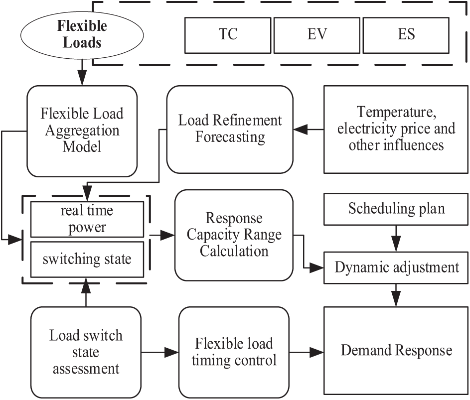
Figure 3: The load aggregation control framework considering dynamic demand response

5  Refined Prediction of Flexible Loads Based on SSA-BiLSTM

5.1 BiLSTM Model

Long Short-Term Memory Neural Networks (LSTM) are based on Recurrent Neural Networks (RNN), introducing Constant Error Carousel units (CEC) to solve the “gradient disappearance” and “gradient explosion” problems in the BPTT algorithm, and realizes the long-term memory function by increasing structures such as forget gate [37]. It has a good ability of time series analysis. Its basic unit structure is shown in Fig. 4.

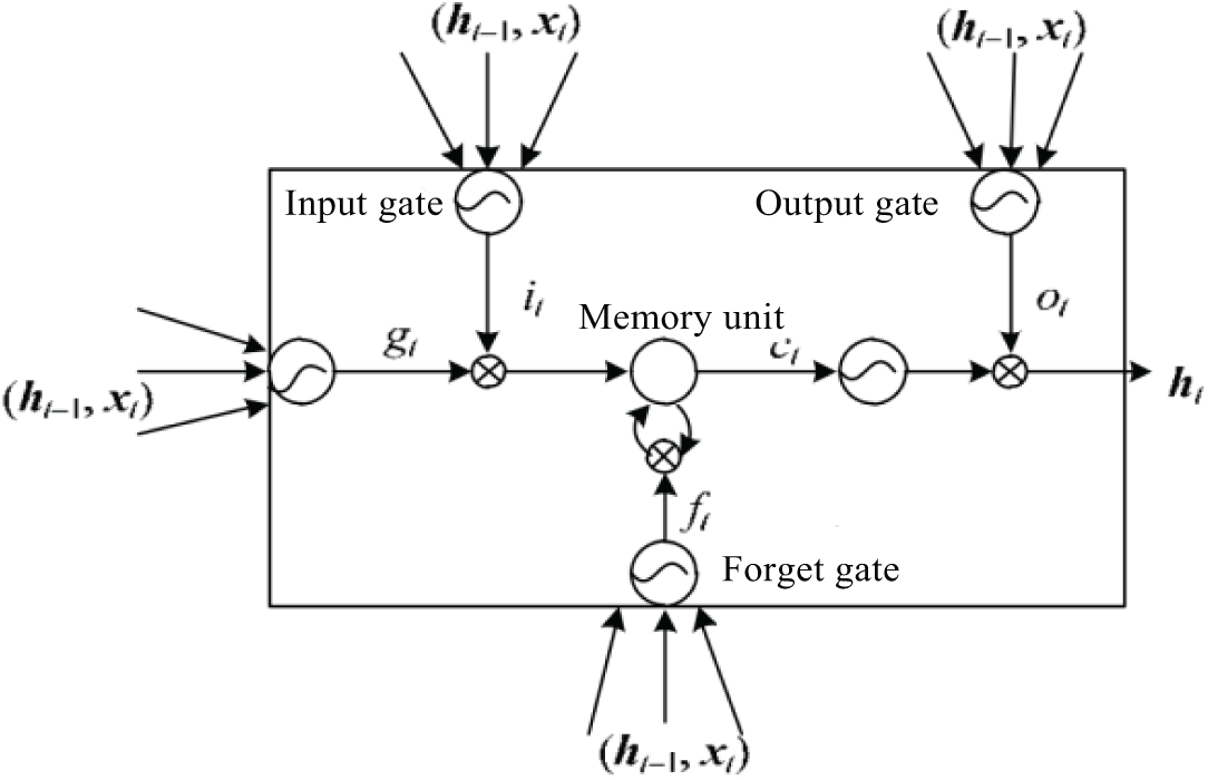
Figure 4: Unit structure of LSTM

As shown in Fig. 4, there are three gates in the basic unit of LSTM: input gate, forget gate and output gate. The input gate is used to update the state of the basic unit, the forget gate determines whether to discard or retain information, and the output gate determines the output information according to the unit state.

The cyclic state of the LSTM basic unit can be expressed as:

ht=f(ht−1,xt)(17)

where ht represents the hidden layer state at time t, xt represents the input vector value at time t.

By introducing the above gates into the cyclic function f, the state iteration update of the LSTM basic unit is calculated as follows:

it=σ(Wi[ht−1,xt]+bi)(18)

ft=σ(Wf[ht−1,xt]+bf)(19)

ot=σ(Wo[ht−1,xt]+bo)(20)

gt=tanh⁡(Wg[ht−1,xt]+bg)(21)

Ct=ftCt+itgt(22)

ht=otCt+tan⁡Ct(23)

where it, ft and Ot are the states of the input gate, forget gate, and output gate, respectively, W and b are the parameters of the LSTM basic unit, Ct is the current state of the basic unit, and gt is the new candidate value of the state of the basic unit.

In time series prediction, the LSTM model mainly deals with unidirectional data information. In order to more effectively capture the dependencies between sequences, BiLSTM introduces forward and backward LSTMs to process forward and backward data flows, respectively [38], and the model structure is shown in Fig. 5.

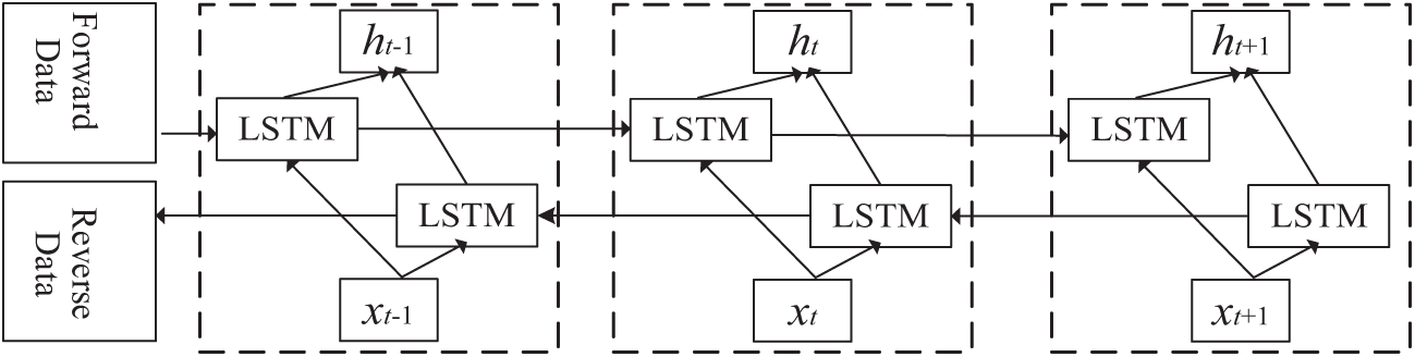
Figure 5: BiLSTM Model structure

As shown in Fig. 5, xt and xt+1 are the input information at time t and t + 1, respectively, and yt and yt+1 are the output information at time t and t + 1, respectively. BiLSTM reduces the risk of under-fitting through the weight sharing mechanism, which not only does not increase the amount of data required by the model but also has a prediction performance far superior to LSTM.

5.2 Model Parameter Optimization Method Based on SSA

To avoid relying on researchers’ experience for selecting key parameters and falling into local optima, the Sparrow Search Algorithm (SSA) is used in this paper to optimize the key parameters of BiLSTM, and the steps are shown in Fig. 6.

Figure 6: Optimisation process of SSA

SSA mainly realizes position optimization by imitating the foraging and anti-predation behavior of sparrows, thus finding the local optimum for some nonlinear optimization problems [39]. The process is as follows:

1.    Initialize the sparrow population: The population consists of n sparrows. If the dimension of the variables to be optimized is m, then the population can be represented as:

X=[x1,1x1,2…x1,mx2,1x2,2…x2,m⋮⋮…⋮xn,1xn,2…xn,m](24)

where xi = (xi1, xi2, … , xim) is the position of the i-th sparrow.

2.    Calculate the fitness and sort: Sparrows with strong adaptability will preferentially obtain food, and at the same time, they will also attract other individuals to join and expand the search range. The corresponding fitness is expressed as:

FX=[f([x1,1,x1,2,…x1,m])f([x2,1,x2,2,…x2,m])⋮f([xn,1,xn,2,…xn,m])](25)

3.    Update the position of the discoverers: The discoverers continuously update their positions, and the iterative process can be expressed as:

Xi,jd+1={Xi,jdexp⁡(−iα⋅itermax)R2<STXi,jd+QR2≥ST(26)

where Xi,jd is the current position of the discoverer, d is the iteration number, α is a random number, β is the maximum iteration number, Q is a random number obeying the normal distribution, L is the alarm value, and S is the safety value.

4.    Update the position of the joiners: When the discoverer finds better food, other sparrows will join in the scramble. If the scramble is successful, they will become joiners and update their positions, which can be expressed as:

Xi,jd+1={Q⋅exp⁡(Xworstd−Xi,jdi2)i>n2Xpd+1+|Xi,jd−Xi,jd|A+1≤i≤n2(27)

where Xworstd is the global worst position, and XPd+1 is the best position of the discoverer in the iteration. When i>n/2, it means that the adaptability of the i-th joiner is poor, and it needs to fly to other places to forage.

5.    Update the position of the vigilant sparrows: In the sparrow group, there is a group of vigilant sparrows who will perceive the threats around them. They will inadvertently be vigilant and protect their own group.

Xi,jd+1={Xbestd+β|Xi,jd−Xbestd|fi>fgXi,jd+K|Xi,jd−Xi,jd|fi−fw+εfi=fg(28)

where Xbestd is the current global optimal position, β is the step length control parameter, fi and fg is the adaptation value of the current sparrow position and the global optimal position, fw is the global worst adaptation value, and K is a random number in [−1, 1], the noise ε is close to 0.

6.    Calculate the fitness value and update the sparrow position, judge whether the stop condition is met. If it is met, exit and output the result; otherwise, repeat steps 2–6.

5.3 Refined Prediction Process of Flexible Loads Considering Multiple Factors

Through the generalized model of flexible load aggregation, it can be known that the load size in the time domain is related to variables such as historical load and temperature. In addition, demand-side regulation can also be participated in through measures such as price signals and incentive mechanisms. Considering the above factors, a refined prediction process of flexible loads based on SSA-BiLSTM is constructed, as shown in Fig. 7.

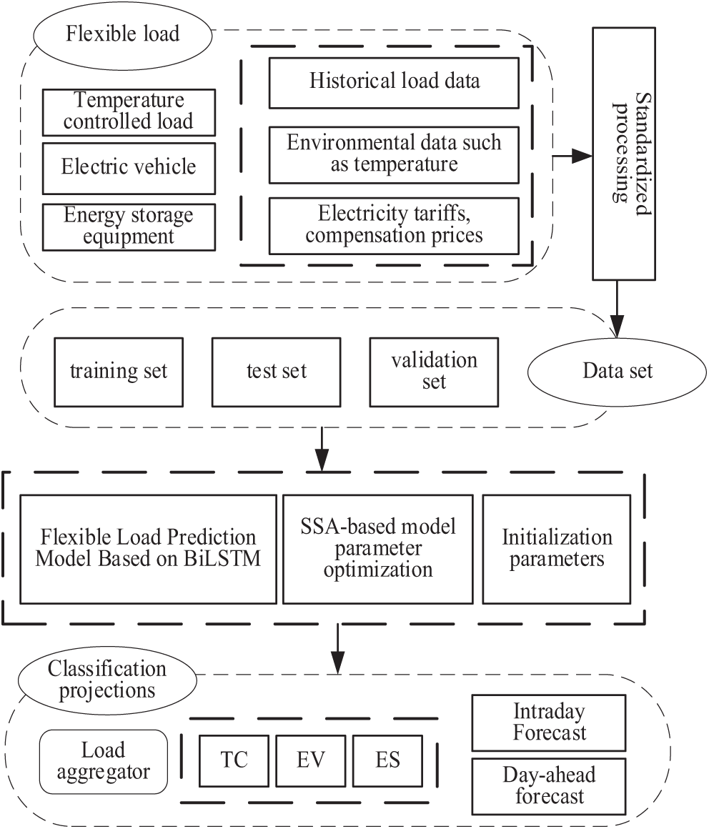
Figure 7: Load forecasting based on SSA-BiLSTM

6  Control of Flexible Load Clusters Based on Parallel MC

6.1 Markov Chain Model

The Markov chain (MC) model believes that the state transition probability is directly related to the current state, and the state transition is a discrete event random process [40]. Assuming that the three states of the Markov chain are Q1, Q2, and Q3, then the state transition probability is shown in Fig. 8.

Figure 8: Markov chain state transfer process

As shown in Fig. 8, assuming that the state at time t is known as Q2, if the state at time t + 1 is Q1, then the state transition probability is A21; if it is Q2, then the state transition probability is A22; if it is Q3, then the state transition probability is A23.

If the three states are randomly converted, the corresponding state transition probability matrix can be expressed as:

A=[A1,1A1,2A1,3A2,1A2,2A2,3A3,1A3,2A3,3](29)

If a state transition probability matrix is used to describe the transitions between N states, the probability of moving from state i to state j is represented by the elements Tij in the matrix, as follows:

T=[T1,1T1,2…T1,NT2,1T2,2…T2,N⋮⋮…⋮TN,1TN,2…TN,N](30)

The state transition probability matrix T satisfies the following three properties:

1.    Non-negativity: The elements in matrix T are non-negative numbers, and the sum of each row is 1, that is:

∑j=1NTi,j=1(31)

2.    Memorylessness: The next state is determined only by the current state and is irrelevant to the states before this time, that is, the conditional probability satisfies:

p{x(t+1)|x(1),x(2),…,x(t)}=p{x(t+1)|x(t)}(32)

3.    Convergence: No matter what the initial state is, as long as the state transition matrix T does not change, after enough transitions, the final state will always converge to a fixed value, that is:

limn→∞x(t)⋅TN×Nn=limn→∞y(t)⋅TN×Nn(33)

where x(t) and y(t) represent different initial states, and TN×Nn represent infinite transformations.

6.2 Assessment of Switching State Transition Probability of Flexible Loads

Since the start-stop state of temperature-controlled loads, electric vehicles, and energy storage devices dynamically converts within different time scales, it belongs to a typical random discrete process. Therefore, according to the Markov chain model, the state transition probability matrix can be constructed to assess the switch state of flexible loads in different time periods.

Taking energy storage devices as an example, the start-stop state transition probability matrix is as follows:

TES=[sES|s=−1→−1sES|s=−1→0sES|s=−1→1sES|s=0→−1sES|s=0→0sES|s=0→1sES|s=1→−1sES|s=1→0sES|s=1→1](34)

Under the condition of obtaining sufficient historical data of load switch start-stop state, this paper replaces the probability with the state transition frequency of different flexible loads within a certain time scale, and then combines the maximum likelihood estimation and conditional probability to construct the transition probability matrix, that is:

p{S(t+1)=j|S(t)=i}=p{S(t)=i∩S(t+1)=j}p{S(t)=i}(35)

A single hidden Markov model cannot meet the vector analysis of the start-stop state of multiple types of loads, so the parallel Markov model is introduced to improve the efficiency of the start-stop state assessment of flexible loads, and its decision process is shown in Fig. 9.

Figure 9: Switching state assessment for flexible loads

According to property 3 of the state transition probability matrix T, after enough times of transition, the probability corresponding to the start-stop state of the flexible load will converge to a fixed value, which is irrelevant to the initial state. Therefore, the convergence value of the switch start-stop state transition probability can be used as the switch state assessment value of the flexible load, and based on the calculation method of the response capacity of the flexible load aggregation and the refined prediction result of the flexible load, the upper and lower limit values of the adjustable capacity of the load aggregator can be further calculated.

6.3 Sequence Control of Flexible Loads Based on Flood Fill Algorithm

The Flood Fill Algorithm (FFA) is simply like a flood first flowing to the low-lying areas and then diffusing to the nearby connected areas until the entire connected area is filled. It is commonly used in the fields of computer networks and graphics processing [41].

The implementation method of the FA algorithm fully utilizes the spatiotemporal correlation of the target trajectory, prioritizes the measurement range from two aspects of spatial distance and time interval, gradually carries out similarity measurement, and divides the measurement range into source point measurement and node measurement according to the degree of priority. The “peak-valley” capacity is allocated first, and then it diffuses to the nearby connected areas. The process is shown in Fig. 10.

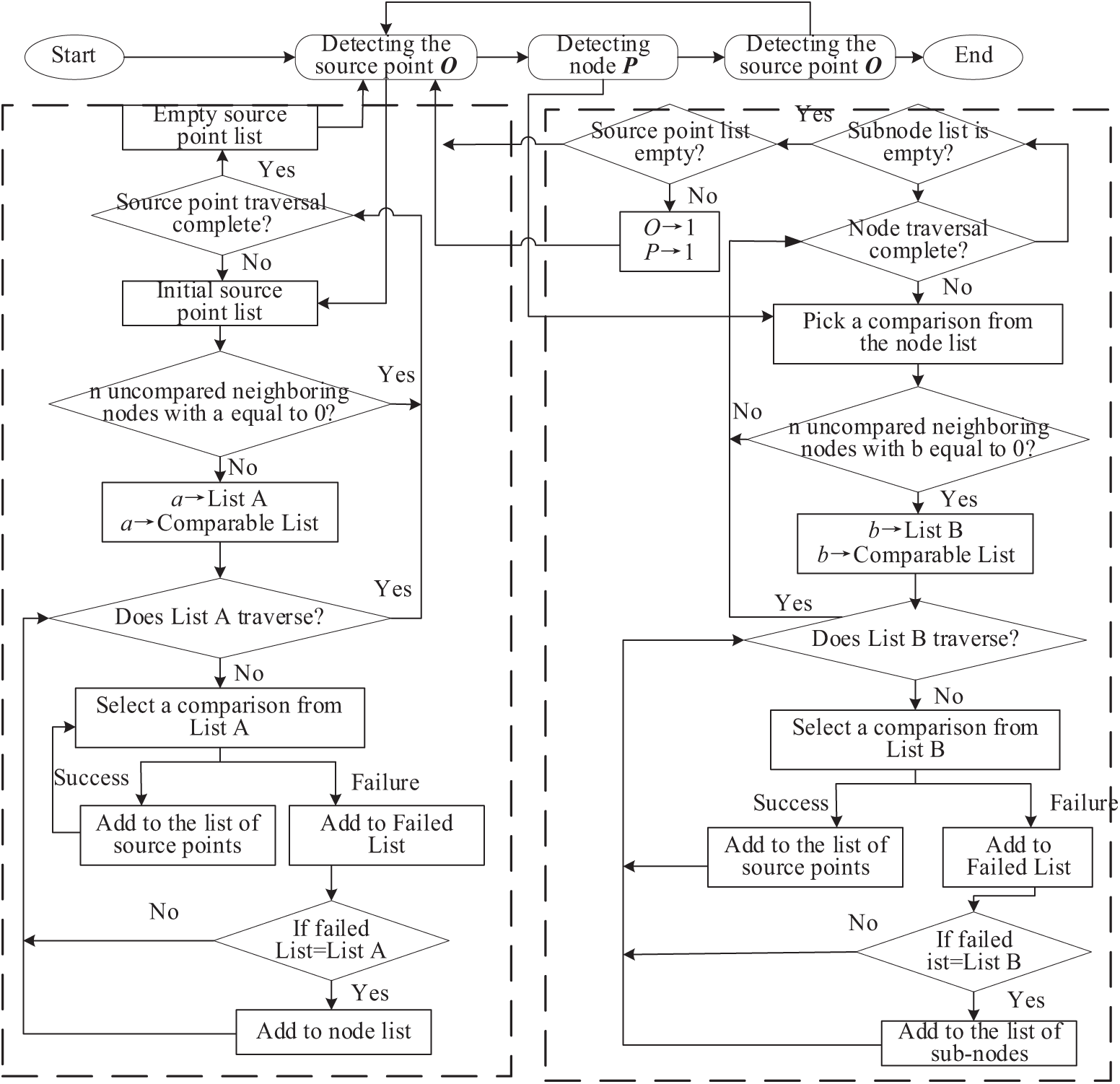
Figure 10: Flow of FFA algorithm

As shown in Fig. 10, three steps need to be performed in sequence.

1.    Select a source in turn from the source list, calculate the n nodes closest to the source O based on the feature similarity, if any node is above the threshold, add that node to the source list; if all n nodes are below the threshold, divide the source O to the node list, and then select the next source in turn from the source list until the source list is traversed and the metric is completed;

2.    Select a node P from the node list in turn, calculate the n nodes nearest to that node P and perform the metric in turn, if all nodes are metric successful, then add the node to the source node list, otherwise add the node to the secondary node list, eventually all nodes will be added to the source list and secondary node list, respectively;

3.    Check the source point list and the node list separately until both lists are cleared, meaning no new nodes can be calculated within the specified area.

7  Case Analysis

7.1 Model Parameter Configuration

Taking Shanxi Province as an example, select a load aggregator, which is set up with 3 load agents. Each load agent is configured with different proportions of flexible loads, and the user behavior is independent, as shown in Table 1.

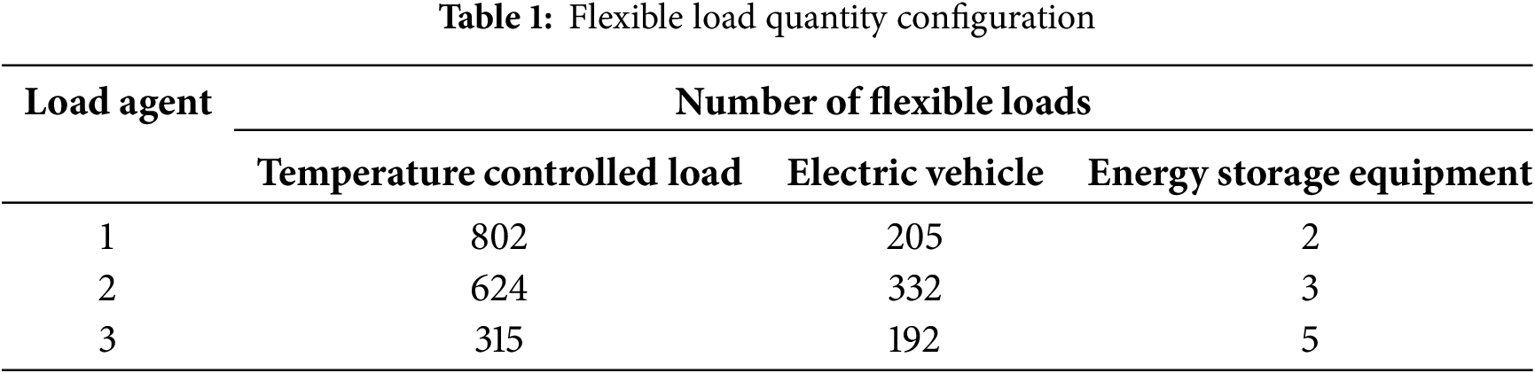
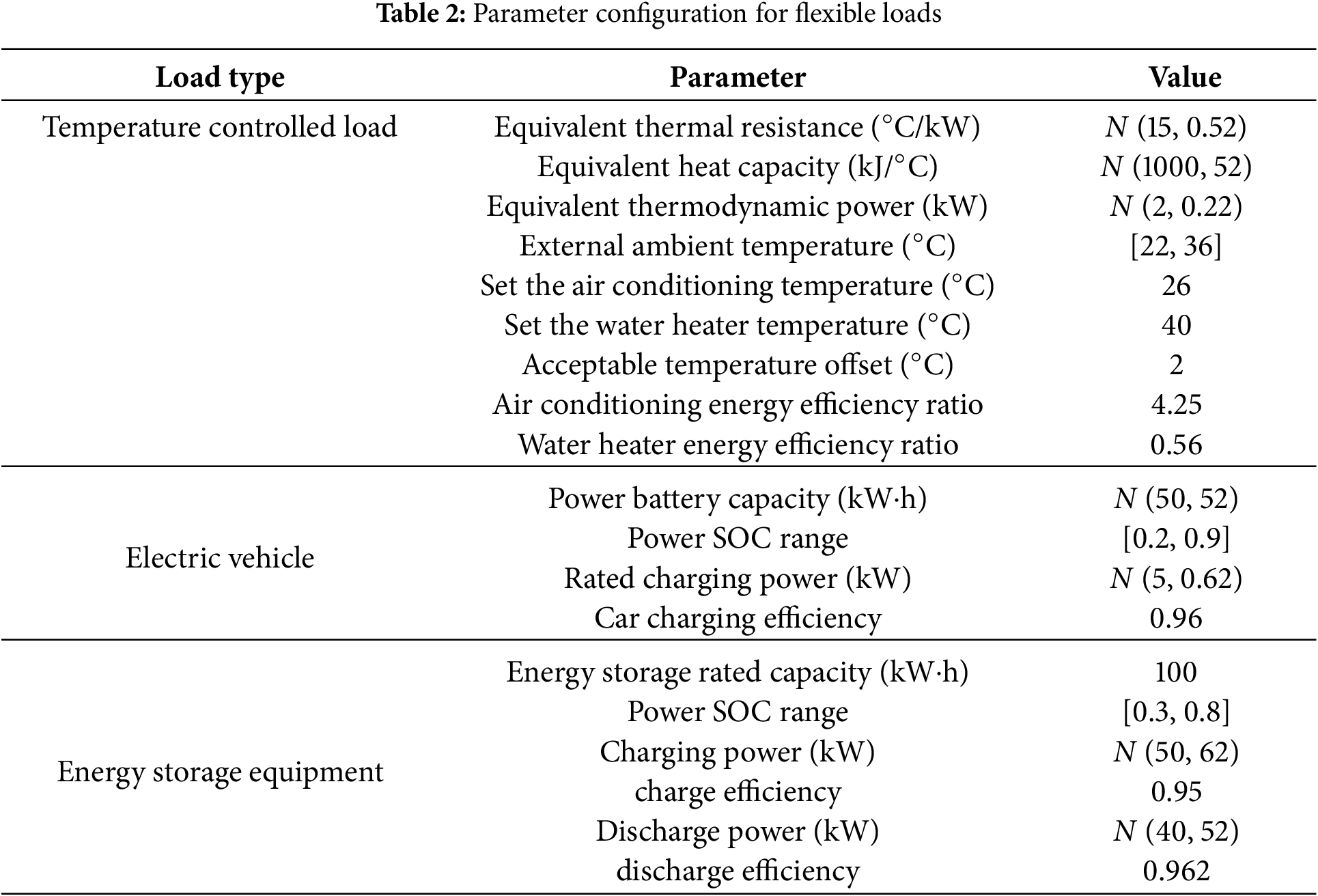
In this case, the relevant parameters of temperature-controlled loads, electric vehicles, and energy storage devices are shown in Table 2.

7.2 Analysis of Flexible Load Prediction Results

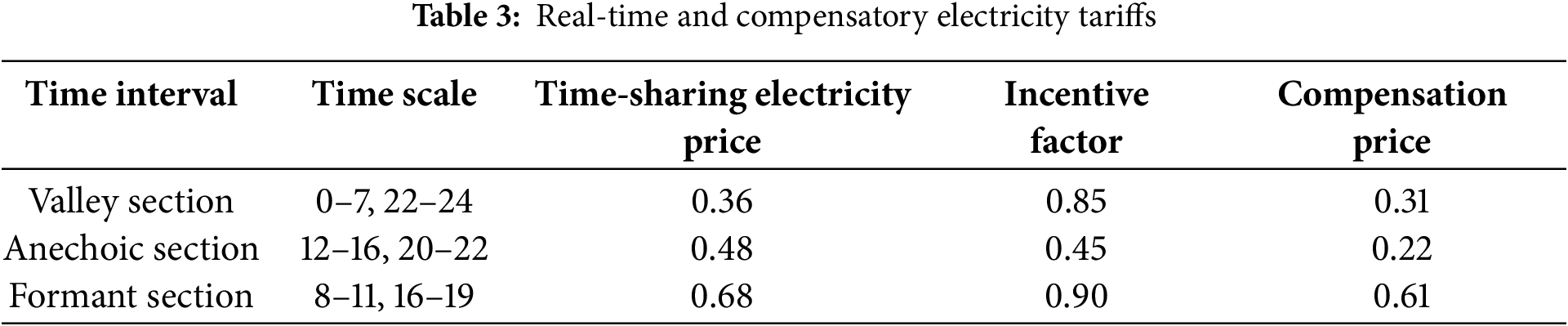
The load prediction model carries out “sliding window” processing on the historical load, temperature, electricity price, incentive, and other time series data in the input part. It then predicts the above three types of loads in the output part, respectively. The electricity price adopts the time-of-use electricity price strategy, and the incentive coefficients for flexible loads to participate in load regulation in different time periods are different and the compensation electricity prices (yuan/kW·h) are also different, as shown in Table 3.

7.2.1 Day-Ahead Prediction Results Analysis for Load Agents

Taking the 3 load agents as objects, the day-ahead load prediction is carried out for the three types of flexible loads: temperature-controlled equipment, electric vehicles, and energy storage devices. After cumulative summation, the total load of the day is formed, and the time granularity is set to 1 h. The load prediction results are shown in Fig. 11.

Figure 11: Day-ahead load forecast results for load agent

Combining Fig. 11 and Table 1, it can be seen that there are typical differences in the composition and power change trend of flexible loads of the above 3 load agents. Among them, the total load of Agent 1 shows “double peak” characteristics, which is related to the high capacity of temperature-controlled loads, and the peak-valley period is basically consistent with Table 3; the total load of Agent 2 shows “valley” characteristics, which is related to the increase of electric vehicle capacity, and the load peak is in the evening; the total load of Agent 3 also shows “valley” characteristics, but the peak-valley difference is significantly enlarged, which is related to the increase of energy storage capacity, and the load peak is concentrated in the night and early morning.

7.2.2 Intraday Prediction Results Analysis for Load Aggregator

1. Classification Aggregation Prediction Results of Flexible Loads

Taking the load aggregator as the object, the various types of flexible loads of the load agents are aggregated, and then the intraday load prediction is carried out. The time granularity is set to 15 min, and the intraday prediction results of the three typical flexible loads are shown in Fig. 12.

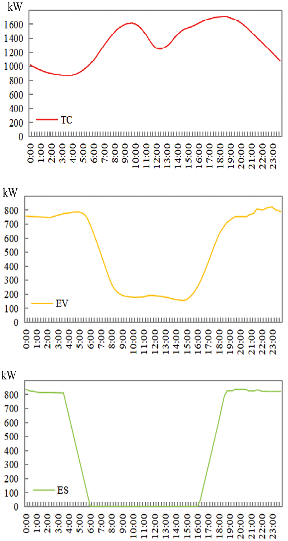
Figure 12: Intraday load forecast for different FL

As shown in Fig. 12, the change curves of the three typical flexible loads show different characteristics. The curve of temperature-controlled load shows a more obvious “double peak” characteristic, and the peak load is concentrated at the peak time of 9:00 and 18:00, which is close to the time of going to and from work, indicating that the temperature-controlled load is closely related to user behavior; the curve of electric vehicle load shows a more significant “wave valley” characteristic, with low load from 7:00 to 16:00 in the daytime and small fluctuations in the evening load, indicating that it is easily affected by the high daytime vehicle usage demand and the cheap evening charging electricity price; the curve of energy storage device load shows an “inverted trapezoidal” characteristic, with almost no load from 7:00 to 16:00 in the daytime, but the evening load is relatively stable, indicating that it has fully stored energy in the valley period for self-use in the daytime or charging other equipment.

2. Total Load Prediction Results of Aggregator

As shown in Fig. 13, the total load prediction results of the aggregator obtained after flexible load aggregation show a “single peak” characteristic, indicating that the electric vehicles have reached a certain load capacity, which has a hedging effect on the first “peak” of the temperature-controlled load. In addition, the energy storage device has a high load in the valley period, which further smooths the “valley” characteristic of the temperature-controlled load.

Figure 13: Intraday forecast results for LA

7.2.3 Comparison Analysis of Different Flexible Load Prediction Algorithms

Taking the temperature-controlled load as an example, the LSTM, BiLSTM, and SSA-BiLSTM algorithms are used for intraday prediction, and the load curves are shown in Fig. 14.

Figure 14: Comparison of load forecasting results

It’s hard to tell which model performs better. Thus, it’s necessary to calculate the difference between the model’s predicted results and the actual values and add another plot, similar to Fig. 15, to show the error sequence.

Figure 15: Comparison of load forecasting error results

As shown in Fig. 15, all three algorithms have a good prediction effect, but the fluctuation deviation of the LSTM prediction curve is large. At the same time, the prediction curves of BiLSTM and SSA-BiLSTM algorithms are smoother and closer to the actual load curve.

In order to further compare the different effects of the three algorithms, the standard deviation of the predicted values and the true values at 96 moments of the day is statistically distributed, as shown in Fig. 16.

Figure 16: Standard deviation of prediction results of different algorithms

As shown in Fig. 16, the standard deviations of the predicted values of the LSTM, BiLSTM, and SSA-BiLSTM algorithms decrease in turn, indicating that the SSA-BiLSTM algorithm proposed in this paper has better load prediction accuracy. After ten-fold cross-validation, the prediction accuracy is 98.84%.

7.3 Switch State Assessment

Combined with the parallel Markov chain model, the historical state data of a large number of load switches in the cluster are statistically analyzed. The state transition matrix is constructed by approximating the probability with the statistical frequency. Under the condition of a random initial state, after 200 state transitions, the probability converges, and the corresponding switch state sequence probability distribution is shown in Fig. 17.

Figure 17: Load switch state assessment results

As shown in Fig. 17, the switch of different flexible loads shows typical start-stop difference characteristics in different periods. The probability of a temperature-controlled load starting in the two peak periods is 50%–70%, which is obviously higher than that of shutdown. In the valley period (early morning), the probability of shutdown is 40%–90%, which is also obviously higher than that of starting; the probability of electric vehicles starting to charge in the evening valley period is 60%–80%, which is obviously higher than that of idle state, and the probability of starting to charge in the daytime peak period is less than 30%; the probability of energy storage devices starting to discharge in the peak period is 50%–60%, and the probability of starting to charge in the valley period is 70%–80%. In the flat period, the probability of being in an idle state is higher, at 60%–80%.

7.4 Flexible Load Response Capacity

Based on the above refined load prediction and switch state probability assessment results, according to the maximum adjustable capacity calculation method in the load aggregation model, the sequence distribution of the maximum adjustable capacity of the flexible load aggregation is shown in Fig. 18.

Figure 18: Maximum capacity adjustment range for LA

As shown in Fig. 18, the maximum daily adjustment capacity of flexible load aggregators is approximately −2000~2000 kW, but there are some differences in the adjustment capacity at different times. Among them, the peak hour has the greatest potential for capacity adjustment, indicating that the charging and discharging behavior of electric vehicles and energy storage is more flexible during this period, and the demand response speed is faster.

Based on the intraday load prediction results of the aggregator mentioned above, as the baseline load of the day, considering the extreme values of the sequence adjustable capacity, the upper and lower limit values of the total load are further obtained, as shown in Fig. 19.

Figure 19: Upper and lower capacity limits of LA

As shown in Fig. 19, the load aggregator has a more flexible capacity regulation threshold, which can follow the scheduling plan in real time within the safe range of the upper and lower limit values. especially in the peak period, the demand side response potential is the strongest. It shows that compared with traditional dispersed and independent loads, the flexible load aggregator, as a whole, has a better ability to smooth the peak and valley and regulate the load.

7.5 Coordinated Control of Flexible Loads

7.5.1 Day-Ahead Coordinated Control of Flexible Loads

According to the day-ahead scheduling plan and the day-ahead load prediction results mentioned above, the scheduling plan capacity is initially distributed based on the flood fill algorithm proposed in this paper, and the peak and valley period capacity shortages are satisfied preferentially. The initial distribution and sequence control results of the regulation capacity of different flexible loads facing the day-ahead scheduling plan are shown in Fig. 20.

Figure 20: Flexible load day-ahead timing control

As shown in Fig. 20, according to the day-ahead scheduling plan, the scheduling capacity of 24 periods is initially distributed at a time interval of 1 h. Among them, the energy storage device has the highest proportion of distributed capacity in the peak and valley stages, indicating that the energy storage device is more stable, less affected by factors, and has the strongest adjustability; the temperature-controlled load has a higher proportion of distributed capacity in the peak period, but the lowest proportion in the valley period, indicating that the temperature comfort zone of air conditioners and other equipment can be adjusted within a limited range, and there may be significant differences in users’ willingness to adjust due to the large difference in electricity prices in the peak and valley periods; electric vehicles have a higher proportion of distributed capacity in the valley period, and the proportion of distributed capacity in the flat period always remains at a low level, indicating that electric vehicle users are most willing to participate in load regulation in the evening valley period, and are not very sensitive in other periods.

7.5.2 Intraday Coordinated Control of Flexible Loads

Due to the changes in environmental temperature and other reasons, the intraday load prediction and scheduling plan will have small-range changes. The secondary distribution and intraday sequence control results of the flexible load regulation capacity are shown in Fig. 21.

Figure 21: Flexible load intra-day timing control

As shown in Fig. 20, according to the intraday scheduling plan, the scheduling capacity of 96 periods, 4 periods in each hour, is secondarily distributed at a time interval of 15 min. It can be found that the scheduling plan curve has local fine-tuning, but the overall distribution characteristics of the load capacity are similar to the initial distribution, with only slight differences, mainly manifested as more refined load sequence control.

Compared with the scheduling plan curve, under the intraday coordinated control strategy of flexible loads, the real-time scheduling curves of various flexible loads in the day are shown in Fig. 22.

Figure 22: Real-time scheduling curve of flexible load within the day

As shown in Fig. 22, the above three types of flexible loads all actively participate in the load scheduling plan. In terms of regulation capacity, from large to small, they are energy storage devices, temperature-controlled loads, and electric vehicles, which is basically consistent with the previous analysis.

Due to the actual load changes and the influence of external uncertainty factors, the deviation of the regulation capacity in each period of the day is shown in Fig. 23.

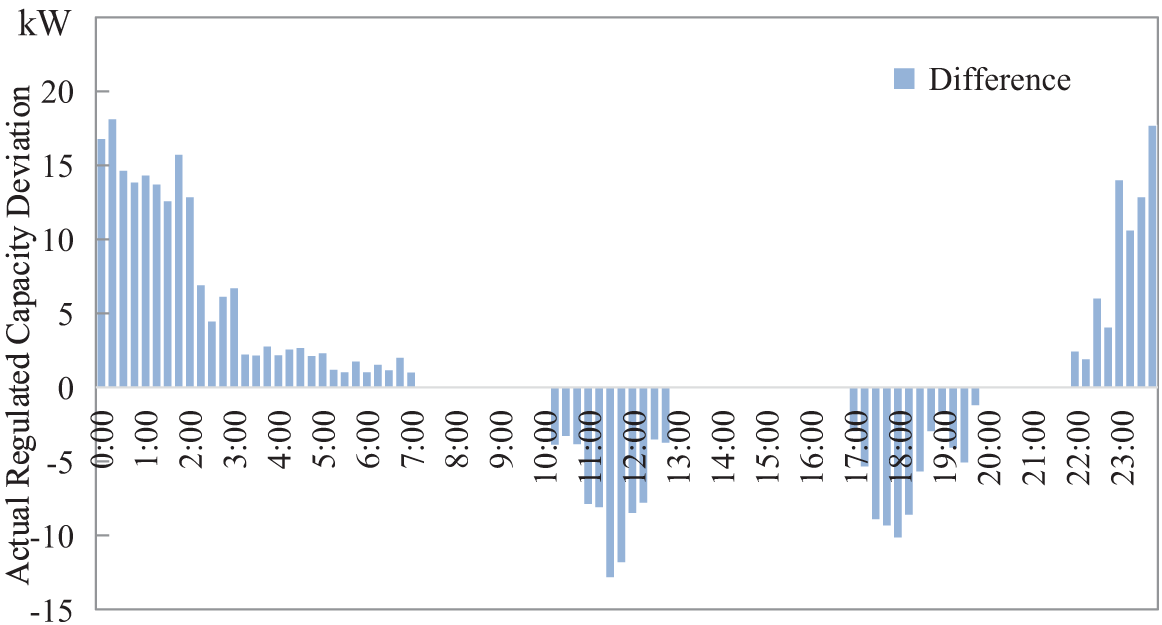
Figure 23: Actual regulated capacity deviation

As shown in Fig. 23, the actual regulated capacity deviation can be traced to multiple factors. During peak and valley periods, the deviation is concentrated due to distinct electricity consumption patterns. Peak hours bring a surge in demand from industrial operations and residential appliance use. The aggregator faces challenges in regulating load for supply-demand balance, as sudden load changes are hard to predict precisely. The relatively small deviation range of around −15 to 20 kW is evidence of the effective control mechanisms. Despite fluctuations, the proposed model maintains deviation within limits, showing its robustness in handling flexible load dynamics.

Social-cultural factors, such as a community’s work culture and hours, impact the deviation significantly. In work-centered communities with long, regular work hours, electricity consumption is concentrated. High commercial-industrial use during work hours and a residential spike in the evening make load prediction and regulation difficult, increasing the deviation. Conversely, in communities with flexible work cultures or many remote workers, consumption is more evenly spread, reducing peak-valley differences and leading to more stable load regulation and smaller deviation.

Future research could focus on quantitatively assessing the impact of various social-cultural factors on regulated capacity deviation. By collecting data from diverse communities, we can establish more accurate correlations. Additionally, exploring innovative control strategies that adapt to these social-cultural variations can enhance the effectiveness of load regulation. We might also study how to better integrate real-time social-cultural data into load-forecasting models, enabling more precise predictions and minimizing capacity deviation.

8  Conclusion

This paper proposes a multivariate, heterogeneous, flexible load aggregation control method oriented to dynamic demand response. The main conclusions are as follows:

1.    The flexible load prediction model based on SSA-BiLSTM fully considers external factors such as temperature and electricity price and can carry out day-ahead and intraday predictions with different time granularity according to needs, and the intraday prediction accuracy reaches 98.84%.

2.    The parallel Markov chain model can effectively assess the switch state of flexible loads, and then based on the generalized modelling of time-domain aggregation of flexible loads and the calculation method of maximum adjustable capacity, combined with the load prediction results, the maximum capacity of increased and decrease of various types of flexible loads is obtained, which provides support for the load aggregator to participate in the scheduling plan.

3.    Combined with the day-ahead and intraday scheduling plans, the flood fill algorithm can be used to carry out the initial and secondary distribution of the flexible load response capacity and carry out refined sequence control, respectively, so as to realize dynamic demand response, and the deviation capacity is controlled within 5%.

4.    Despite the promising results, the proposed models in this study have several limitations. The SSA-BiLSTM flexible load prediction model, while accounting for temperature and electricity price, may not capture all influencing factors. Sudden economic policy changes or large-scale events that impact consumption patterns are overlooked, which could lead to prediction inaccuracies during such events. Additionally, the parallel Markov chain model assumes regularities in flexible load switch states. However, real-world user behaviours can be complex and irregular, violating these assumptions and affecting the accuracy of switch state assessment and maximum adjustable capacity calculation.

5.    In the future, research can focus on two main areas. First, to address the current model’s deviation capacity issue, explore advanced optimization algorithms. For example, develop algorithms that adaptively adjust parameters based on real-time load changes to reduce deviation and enhance actual regulation accuracy. Second, consider social-cultural factors. Examine how community work cultures and working hours impact flexible load aggregation. Different work cultures can lead to varied residential electricity consumption patterns. Integrating these variables into the model will improve its practicality and offer more reliable support for dynamic demand response across diverse social scenarios.

Acknowledgement: We would like to express our gratitude to the reviewers and editors for their valuable comments and suggestions. We also extend our sincere thanks to all individuals and organizations that have provided support during the research process.

Funding Statement: This research was funded by the Science and Technology Project of State Grid Shanxi Electric Power Co., Ltd., with the project number 52051L240001.

Availability of Data and Materials: The data that support the findings of this study are available on request from the corresponding author, Chun Xiao, upon reasonable request.

Ethics Approval: Not applicable.

Conflicts of Interest: The author declares no conflicts of interest to report regarding the present study.

References

1. Ding P, Deng T, Ma C, Zhang G, Liu J, She J, et al. Research on the collaborative evolution technology path of standard essential patents for new power systems. In: 2023 13th International Conference on Power and Energy Systems (ICPES); 2023 Dec 8–10; Chengdu, China. p. 598–602. doi:10.1109/ICPES59999.2023.10400150. [Google Scholar] [CrossRef]

2. Qi B, Zheng S, Sun Y, Li B, Tian S, Shi K. A model of incentive-based integrated demand response considering dynamic characteristics and multi-energy coupling effect of demand side. Chin J Electr Eng. 2022;42(5):1783–99. doi:10.13334/j.0258-8013.pcsee.202351. [Google Scholar] [CrossRef]

3. Jiang T, Li Y, Ju P, Yang YA, Zhao J. Overview of modeling method for flexible load and its control. Intell Power. 2020;48(10):1–8. [Google Scholar]

4. Xie H, Luo Y, Su Y, Guo Z, Xu G, Li P, et al. Active support technique for flexibility and stability of multi-partition power grid based on flexible DC control. In: 2024 Boao New Power System International Forum—Power System and New Energy Technology Innovation Forum (NPSIF); 2024 Dec 8–10; Qionghai, China. p. 535–43. doi:10.1109/NPSIF64134.2024.10883276. [Google Scholar] [CrossRef]

5. Kumar S, Sagar HK, Agrawal A. Economical demand-side management with distributed energy resources. In: 2024 IEEE Region 10 Symposium (TENSYMP); 2024 Sep 27–29; New Delhi, India. p. 1–6. doi:10.1109/TENSYMP61132.2024.10752266. [Google Scholar] [CrossRef]

6. Sharif AA, Karegar HK, Beigi SE. Intelligent fault detection and location method for DC micro-grid by considering different fault and non-fault operation modes. In: 2023 13th Smart Grid Conference (SGC); 2023 Dec 5–6; Tehran, Iran. p. 1–7. doi:10.1109/SGC61621.2023.10459315. [Google Scholar] [CrossRef]

7. Yang WJ, Yin XQ, Tao J, Zhang HY. Fault current constrained impedance-based method for high resistance ground fault location in distribution grid. Electr Power Syst Res. 2024;227(06):109998. doi:10.1016/j.epsr.2023.109998. [Google Scholar] [CrossRef]

8. Flygare C, Jonasson E, Åberg M, Castellucci V. The value of now, later, or never: assessing the value of electricity users’ flexibility. In: CIRED 2024 Vienna Workshop; 2024 Jun 19–20; Vienna, Austria. p. 1063–6. doi:10.1049/icp.2024.1948. [Google Scholar] [CrossRef]

9. Xin YC, Li GQ, Wang Y, Ling W. The compensation control of reactive power and three phase unbalance load based on the method of sequence component. In: 2012 China International Conference on Electricity Distribution; 2012 Sep 10–14; Shanghai, China. p. 1–5. doi:10.1109/CICED.2012.6508492. [Google Scholar] [CrossRef]

10. Ahmed MT, Hassan MR, Ghosh PC, Huq MS, Islam M, Nazmul Huda AS. Monte Carlo simulation for reliability worth assessment of distribution system considering momentary interruptions. In: 2022 International Conference on Energy and Power Engineering (ICEPE); 2022 Nov 24–26; Dhaka, Bangladesh. p. 1–6. doi:10.1109/ICEPE56629.2022.10044904. [Google Scholar] [CrossRef]

11. Choi G, Park J, Shlezinger N, Eldar YC, Lee N. Split-KalmanNet: a robust model-based deep learning approach for state estimation. IEEE Trans Veh Technol. 2023;72(9):12326–31. doi:10.1109/TVT.2023.3270353. [Google Scholar] [CrossRef]

12. Xia N, Deng J, Zheng T, Zhang H, Wang J, Peng S, et al. Fuzzy logic based network reconfiguration strategy during power system restoration. IEEE Syst J. 2022;16(3):4735–43. doi:10.1109/jsyst.2021.3123325. [Google Scholar] [CrossRef]

13. Yang X, Fu G, Liu F, Tian Y, Xu Y, Chai Z. Potential evaluation and control strategy of air conditioning load aggregation response considering multiple factors. Grid Technol. 2022;46(2):699–714. [Google Scholar]

14. Liu S, Zhang Z, Chen Y, Hu L. A control strategy of thermostatically controlled loads for power system frequency regulation. In: 2023 IEEE/IAS Industrial and Commercial Power System Asia (I&CPS Asia); 2023 Jul 7–9; Chongqing, China. p. 473–8. doi:10.1109/ICPSAsia58343.2023.10294385. [Google Scholar] [CrossRef]

15. Wei C, Wang Y, Wang C, Xu J, Liao S, Wang J. Real-time linearized scheduling model for distribution networks with aggregated thermostatically controlled loads. In: 2022 4th Asia Energy and Electrical Engineering Symposium (AEEES); 2022 Mar 25–28; Chengdu, China. p. 114–20. doi:10.1109/AEEES54426.2022.9759673. [Google Scholar] [CrossRef]

16. Ma K, Jiao Z, Yang J. A hierarchical scheduling strategy of thermostatically controlled loads in smart grid. In: 2020 IEEE 16th International Conference on Control & Automation (ICCA); 2020 Oct 9–11; Singapore. p. 1278–83. doi:10.1109/icca51439.2020.9264411. [Google Scholar] [CrossRef]

17. Yang T, Zhang H, Wu M, Tang X. Research on the optimization strategy of electric vehicle charging and discharging scheduling. In: 2023 3rd Power System and Green Energy Conference (PSGEC); 2023 Aug 24–26; Shanghai, China. p. 455–9. doi:10.1109/PSGEC58411.2023.10255953. [Google Scholar] [CrossRef]

18. Zhang J, Wang W, Wang R, Li T, Zhao X, Li J, et al. An electric vehicle scheduling strategy for the power grid peak regulation based on V2G. In: 2023 3rd International Conference on New Energy and Power Engineering (ICNEPE); 2023 Nov 24–26; Huzhou, China. p. 1181–7. doi:10.1109/ICNEPE60694.2023.10429591. [Google Scholar] [CrossRef]

19. Li S, Xu Z, Yu L, Du L, Yue L, Zhang X, et al. A load control user combination optimization method with electric vehicle and temperature control load cluster. China Electr Power. 2025;3:86–97. [Google Scholar]

20. Xie D, Li H, Li S, Dai W, Li P. EV aggregation method considering flexibility of multiple charge-discharge modes. In: 2022 2nd International Conference on Electrical Engineering and Control Science (IC2ECS); 2022 Dec 16–18; Nanjing, China. p. 453–8. doi:10.1109/IC2ECS57645.2022.10087983. [Google Scholar] [CrossRef]

21. Jian J, Xu Y, Yi Z. An electric vehicle aggregation region approach for active distribution network optimal dispatch. In: 2022 IEEE/IAS Industrial and Commercial Power System Asia (I&CPS Asia); 2022 Jul 8–11; Shanghai, China. p. 1765–70. doi:10.1109/ICPSAsia55496.2022.9949822. [Google Scholar] [CrossRef]

22. Wang L, Yan Z, Yan H, Liu J, Liu J, Wang Y. Load aggregation method for electric vehicle based on SOM neural network clustering. In: 2023 IEEE/IAS Industrial and Commercial Power System Asia (I&CPS Asia); 2023 Jul 7–9; Chongqing, China. p. 908–12. doi:10.1109/ICPSAsia58343.2023.10294770. [Google Scholar] [CrossRef]

23. Zhuang J, Wang C, Cheng Q, Dai Y, Ghaderpour E, Mohammadzadeh A. Stabilizing electric vehicle systems using proximal policy-based self-structuring control. Int J Automot Technol. 2024;25(6):1485–502. doi:10.1007/s12239-024-00134-3. [Google Scholar] [CrossRef]

24. Zhang X, Hu W, Sun S, Zhou G, Cheng Y, Wang S. A distributed energy storage aggregation method considering power system dispatching requirements and SOC equilibrium. In: 2023 IEEE 18th Conference on Industrial Electronics and Applications (ICIEA); 2023 Aug 18–22; Ningbo, China. p. 816–21. doi:10.1109/ICIEA58696.2023.10241839. [Google Scholar] [CrossRef]

25. Zhang Q, Xu M, Shang B, Ge Y, Fu D, Xie J. Distributed energy storage optimal scheduling in distribution network based on the K-means algorithm. In: 2022 IEEE 6th Conference on Energy Internet and Energy System Integration (EI2); 2022 Nov 11–13; Chengdu, China. p. 3143–7. doi:10.1109/EI256261.2022.10117126. [Google Scholar] [CrossRef]

26. Liu Y, Sun M, Chen P, Liu L, Ding L, Wen F. Unit commitment based optimal aggregation and control method for energy storage systems. In: 2023 IEEE 7th Conference on Energy Internet and Energy System Integration (EI2); 2023 Dec 15–18; Hangzhou, China. p. 1336–41. doi:10.1109/EI259745.2023.10512450. [Google Scholar] [CrossRef]

27. Chen K, Gao S, Liu Y. Optimization of multi-time-scale peak shaving considering controllable margin of flexible load. Power Constr. 2021;42(4):69–78. [Google Scholar]

28. Yan L, Zhu E, Zheng G, Wang C, Lu C. Optimal scheduling of integrated energy systems considering flexible loads. In: 2023 6th International Conference on Electronics Technology (ICET); 2023 May 12–15; Chengdu, China. p. 823–9. doi:10.1109/ICET58434.2023.10211758. [Google Scholar] [CrossRef]

29. Liu J, Liu H, Zhang Y, Deng J, Hu G, Li W. Day-ahead bidding decision optimization model of load aggregators considering adjustable potential of residential users. Intell Power. 2024;52(2):71–8. [Google Scholar]

30. Huang Q, Yang S, Duan M, Kong Y, Dung Z. Demand response potential prediction method with load data features analysis of user clusters. Power Demand Side Manag. 2024;26(1):16–22. [Google Scholar]

31. Yan SR, Dai Y, Shakibjoo AD, Zhu L, Taghizadeh S, Ghaderpour E, et al. A fractional-order multiple-model type-2 fuzzy control for interconnected power systems incorporating renewable energies and demand response. Energy Rep. 2024;12(4):187–96. doi:10.1016/j.egyr.2024.06.018. [Google Scholar] [CrossRef]

32. Sun Y, Li Z, Xu P, Li B, Qi B, Liu Z, et al. Research on key technologies and development direction of heterogeneous flexible load modeling and regulation. Chin J Electr Eng. 2019;39(24):7146–58. doi:10.13334/j.0258-8013.pcsee.181521. [Google Scholar] [CrossRef]

33. Lei R, Jia R, Zhu C. A fast response control algorithm for flexible load in virtual power plants with differentiated scenarios. In: 2024 International Conference on Artificial Intelligence and Power Systems (AIPS); 2024 Apr 19–21; Chengdu, China. p. 364–7. doi:10.1109/AIPS64124.2024.00080. [Google Scholar] [CrossRef]

34. Wang X, Li F, Dong J, Olama MM, Zhang Q, Shi Q, et al. Tri-level scheduling model considering residential demand flexibility of aggregated HVACs and EVs under distribution LMP. IEEE Trans Smart Grid. 2021;12(5):3990–4002. doi:10.1109/TSG.2021.3075386. [Google Scholar] [CrossRef]

35. Cheng J, Xie X, Xi Y, Ma F, Cui X, Ying L. Research on two-level optimization model of demand side resource aggregation participating in peak shaving. J Wuhan Univ. 2024;57(3):338–47. [Google Scholar]

36. Hou Y, Zhao L, Jiang H, Ji X, Zhao J. Two-layer control framework and aggregation response potential evaluation of air conditioning load considering multiple factors. IEEE Access. 2024;12(19):34435–51. doi:10.1109/ACCESS.2024.3368927. [Google Scholar] [CrossRef]

37. Rubasinghe O, Zhang X, Chau TK, Chow YH, Fernando T, Iu HH. A novel sequence to sequence data modelling based CNN-LSTM algorithm for three years ahead monthly peak load forecasting. IEEE Trans Power Syst. 2024;39(1):1932–47. doi:10.1109/TPWRS.2023.3271325. [Google Scholar] [CrossRef]

38. Guo Y, Li Y, Qiao X, Zhang Z, Zhou W, Mei Y, et al. BiLSTM multitask learning-based combined load forecasting considering the loads coupling relationship for multienergy system. IEEE Trans Smart Grid. 2022;13(5):3481–92. doi:10.1109/TSG.2022.3173964. [Google Scholar] [CrossRef]

39. Zhang J, Zheng J, Xie X, Lin Z, Li H. Mayfly sparrow search hybrid algorithm for RFID network planning. IEEE Sens J. 2022;22(16):16673–86. doi:10.1109/JSEN.2022.3190469. [Google Scholar] [CrossRef]

40. Liu H, Shen H, Hu W, Ji L, Li J, Yu Y. Electric vehicle load forecast based on higher order Markov chain. In: 2023 5th Asia Energy and Electrical Engineering Symposium (AEEES); 2023 Mar 23–26; Chengdu, China. p. 1203–7. doi:10.1109/AEEES56888.2023.10114238. [Google Scholar] [CrossRef]

41. Selva Birunda S, Nagaraj P, Krishna Narayanan S, Muthamil Sudar K, Muneeswaran V, Ramana R. Fake image detection in twitter using flood fill algorithm and deep neural networks. In: 2022 12th International Conference on Cloud Computing, Data Science & Engineering (Confluence); 2022 Jan 27–28; Noida, India. p. 285–90. doi:10.1109/Confluence52989.2022.9734208. [Google Scholar] [CrossRef]