Impedance Reshaping Based Stability Analysis and Stabilization Control for Flexibly Interconnected Distribution Networks

1  Introduction

Under the low-carbon policy, a high proportion of new energy sources, a high proportion of power electronic devices, and flexible loads, among other equipment, are being gradually integrated into the distribution networks on a large scale. Their inherent characteristics such as intermittency, randomness, volatility, and low anti-interference capability will lead to a significant intensification of such features as volatility and imbalance between the source and load in the power system [1–3], which in turn will trigger problems including uneven power distribution among feeders, reduced system stability, and decreased power supply reliability. Flexible interconnected based distribution networks (FIDN), by constructing DC links in traditional AC distribution areas through flexible power electronic technologies, can effectively solve issues related to load imbalance and power quality in distribution networks, which has become a development direction for future flexible distribution networks [4–6].

In FIDN system that incorporates diverse power electronic interfaced sources and loads such as PV, energy storage, and various types of loads, the system stability exhibits significant differences under varying operating conditions. Therefore, it is urgent to carry out research on the operational stability of multi-converter systems and corresponding stability enhancement measures in flexible interconnection systems. In terms of stability analysis, Reference [7] established the impedance model and analysis stability of PV energy storage direct energy router based on flexible interconnection. Reference [8] presented Large-Disturbance Stability Analysis of Flexible Interconnected System of Distribution Areas Considering Load-Balancing. Reference [9] discussed the weak damping characteristics and is prone to low-frequency and high-frequency unstable oscillations of dc distribution network system equipped with a large number of power electronic equipment. Reference [10] presented the T-S Fuzzy Model Based Large-Signal Stability Analysis of DC Microgrid With Various Loads. Reference [11] discussed Large Disturbance Stability Analysis of DC Microgrid with Constant Power Load Based on Sum of Square Programming Estimating Attraction Domain. Reference [12] established a small-signal impedance model of a grid-connected inverter with phase-locked loop (PLL) control in the d–q coordinate system. Based on the developed impedance model, it analyzed the relationship between the PLL control parameters and system stability under weak grid conditions. Additionally, factors such as the negative impedance characteristics exhibited by converters operating in constant power mode will also affect the stable operation of the system [13,14]. In terms of system stabilization control strategies, Reference [15] proposed collaborative transfer operation strategy for flexible interconnected systems considering transient stability. Reference [16] proposed an active damping method based on capacitor voltage feedback for three-phase current-source grid-connected inverters, which effectively suppresses system resonance caused by the filter. Reference [17] defines converters in DC distributed systems as Bus Current Controlled Converters (BCCC) and Bus Voltage Controlled Converters (BVCC), and proposes a simple, practical impedance-based stability assessment criterion for DC distributed power systems. Reference [18] proposes a distributed uniform control strategy for bidirectional interlinking converters to achieve resilient operation of hybrid AC/DC microgrids, which enhances the stability margin and power supply reliability of hybrid AC/DC microgrids under various operating conditions. Based on the above analysis, the previous literature focuses on the operational stability and stability enhancement strategies of a single converter or AC/DC microgrid. The stability analysis model for a FIDN system that incorporates multiple types of elements (including flexible interconnection equipment, constant power loads, and photovoltaic-storage systems) from the perspective of the overall system have not been addressed well, especially on the stability impact mechanism and stability enhancement strategy of the FIDN under the conditions of power transmission changes and constant power load changes.

To address these issues, this paper presents an impedance reshaping based stability analysis and stabilization control to enhance the stability of the interconnected system and improve the system’s dynamic load response capability. The main contribution of this paper can be summarized as follows.

(a)   A small-single based equivalent impedance model of FIDN system, which consists of the flexible interconnection equipment, constant power loads, and photovoltaic-storage systems, is presented, and the total output and input impedances of the DC distribution network are derived.

(b)   The impacts of constant power loads and transmission power variations on the small-signal stability of FIDN system is analyzed through Nyquist stability curves using the impedance ratio criterion.

(c)   An impedance reshaping-based stability enhancement strategy for the FIDN system is proposed, which can significantly improve system stability under constant power loads variations, transmission power variations and voltage sag conditions.

The paper is organized as follows: the second part of this paper introduces small-signal impedance modeling of FIDN system. The third part introduces impedance stability analysis of FIDN System. The fourth part presents impedance reshaping based stabilization control. And the fifth part is present the case study simulation analysis, and the sixth part is the conclusion of this paper.

2  Small-Signal Impedance Modeling of FIDN System

Fig. 1 shows the basic structure of a two-terminal FIDN system, where two voltage source converters (VSCs) form a DC distribution path to connect two AC distribution areas with photovoltaic systems. Through power regulation between the two VSCs, power mutual assistance between the two AC distribution zones can be carried out, thereby realizing the management of heavy overload in the AC distribution areas. Meanwhile, DC elements such as energy storage, photovoltaics, and constants loads are connected in the DC distribution area, enabling efficient DC access and local consumption of photovoltaic-storage systems.

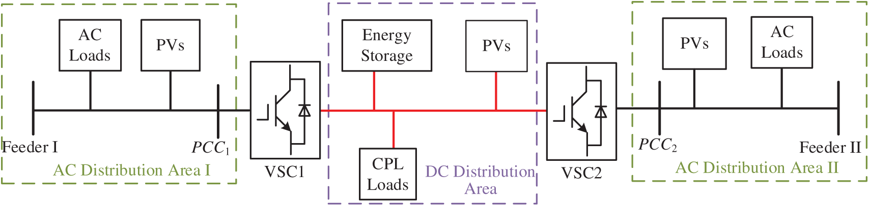
Figure 1: The basic structure of two-terminal FIDN system

When the FIDN system experiences significant fluctuations (e.g., a sudden surge in load or PV system), the transmitted power of the FIDN system accordingly fluctuates. Affected by the control structure or parameter limitations, there is a time delay in the coordinated power control between the two VSC converters. This may lead to instantaneous power surplus (causing overvoltage of the DC bus voltage) or instantaneous power deficit (causing undervoltage of the DC bus voltage), which affects the dc voltage and goes beyond the system’s regulation range. Meanwhile, the negative impedance effect of constant power loads (CPLs) in the distribution area (where the voltage drops, which current increases) can be affected across distribution areas, exacerbating power imbalance. Additionally, fluctuations in the grid impedance on both sides will restrict the regulation capability of the flexible interconnection system, further reduce the stability margin and trigger instability.

In the established DC-side impedance model, the DC-side PV unit is equivalent to a controlled current source, which, together with the VSC, supplies energy to the constant power load (CPL). If the PV output varies and the CPL is consonant, the transmission power of the VSC should be regulated. Therefore, fluctuations in the DC-side PV output can be equivalent to either VSC transmission power variations (with the CPL remaining constant) or fluctuations in the CPL load (with the power transmitted by the VSC kept constant).

Under normal operating conditions, when the flexible interconnection system transmits power between feeders, its primary objective is mostly to balance the load rates across multiple feeders, thereby addressing the issue of feeder overloading. When the output power of PV units on the AC side fluctuates, this can be equivalent to a change in the load of the AC feeder. In such cases, the VSC can adjust the transmitted power in real time to maintain balanced load rates among feeders. Therefore, fluctuations in the AC-side PV output can also be equivalent to fluctuations in the power transmitted by the VSC.

Therefore, the stability analysis and discussion of this paper focuses on the influence mechanisms of the transmitted power of flexible interconnection devices and constant power loads (CPLs) on system stability.

2.1 Model of the Flexibly Interconnected Equipment

Fig. 2 shows the topological structure of the flexible interconnection equipments (FIE). Among them, resistors R1 and R2 are the equivalent resistors on the AC side of converters VSC, respectively. L1 and L2 are the equivalent inductors on the AC side of converters VSC, respectively. C is the DC bus capacitor. ugabc1(2) is the AC voltages on the side of AC distribution area I and II, respectively. ia1(2), ib1(2), ic1(2) are the AC currents on the side of AC distribution area I and II, respectively. ua1(2), ub1(2), uc1(2) are the AC voltages of converters VSC, respectively. udc is the DC side voltage. idc1(2) is the DC side currents of converters VSC respectively. Sa1(2), Sb1(2), Sc1(2) represent the on and off states of the upper bridge arm switching devices, and S′a1(2), S′b1(2), S′c1(2) represent the on states of the lower bridge arm switches.

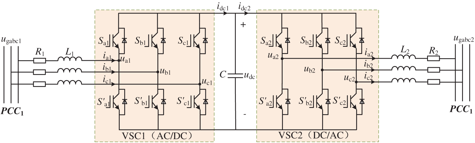
Figure 2: The topological structure of the flexible interconnection equipment

Based on the KLV and KCL functions, the state-space mathematical model of FIE under d-q axis can be expressed as

L1ddt[id1iq1]=[ugd1ugq1]−[R1−ωL1ωL1R1][id1iq1]−[dd1dq1]udc(1)

Cdudcdt=32[dd1dq1][id1iq1]−idc2(2)

L2ddt[id2iq2]=−[ugd2ugq2]−[R2−ωL2ωL2R2][id2iq2]+[dd2dq2]udc(3)

During steady-state operation, the modulation component exhibits a fixed steady-state value. When the system is subjected to a small disturbance, the modulation component generates a small variation around this steady-state value. By linearizing Eqs. (1)–(3) around their steady-state values, neglecting high-order disturbance terms, and performing Laplace transform, the small-signal model of the VSC DC side can be obtained as

sL1[Δid1Δiq1]=[Δugd1Δugq1]−[R1−ωL1ωL1R1][Δid1Δiq1]−[Dd1Dq1]Δudc−[Δdd1Δdq1]Udc(4)

sCΔudc=32[Δdd1Δdq1][Id1Iq1]+32[Dd1Dq1][Δid1Δiq1]−Δidc2(5)

sL2[Δid2Δiq2]=−[Δugd2Δugq2]−[R2−ωL2ωL2R2][Δid2Δiq2]+[Dd2Dq2]Δudc+[Δdd2Δdq2]Udc(6)

where Δ denotes a small disturbance variable, which is used to describe the small variation of a specific physical quantity around the steady-state operating point. And Δd and Δq stand for the small variation value for d-axis and q-axis duty cycle.

The control strategies adopted by converters VSC1 and VSC2 are respectively constant DC voltage-reactive power (VdcQ) control and constant active power-reactive (PQ) power control, and the corresponding diagrams are plots in Fig. 3.

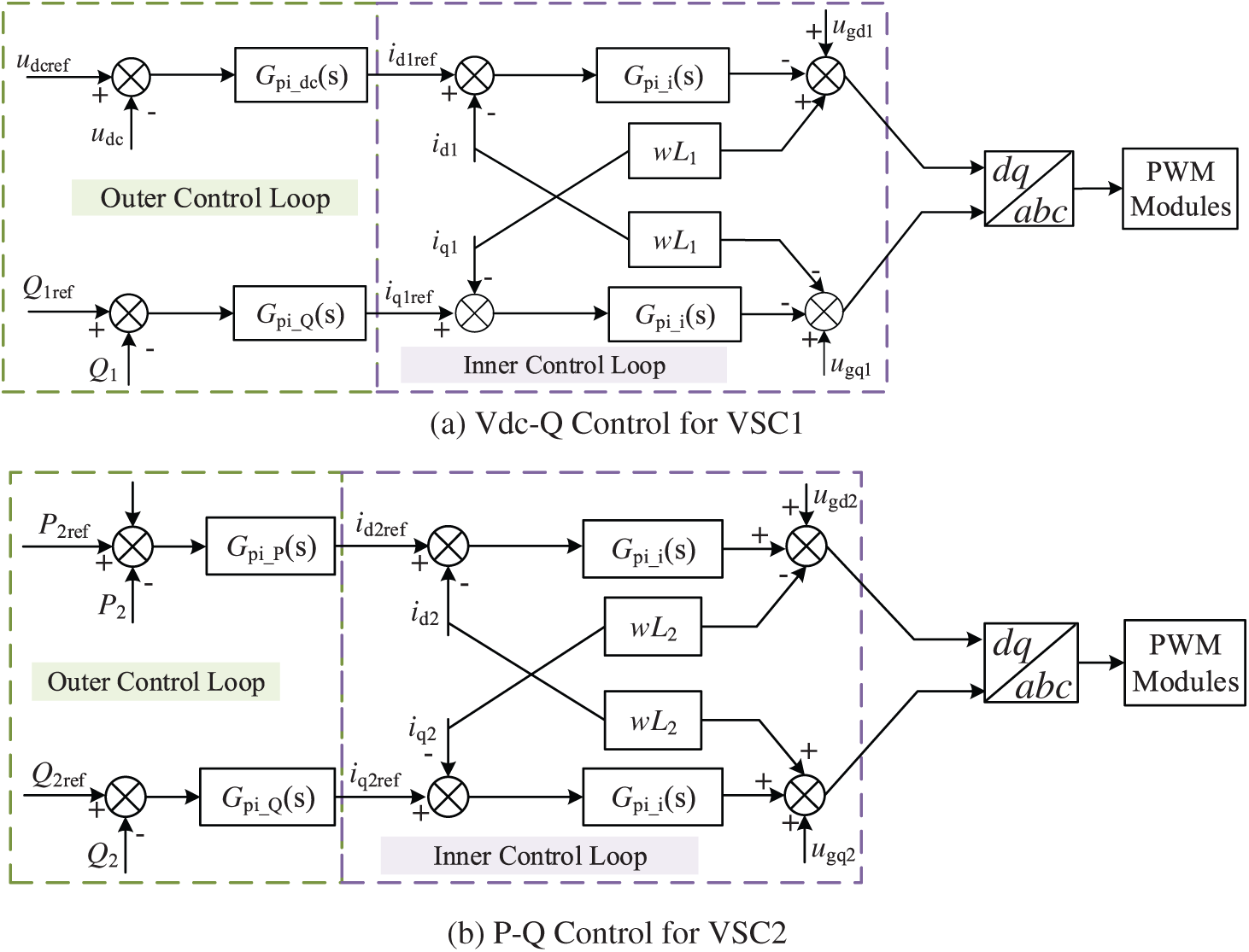
Figure 3: Control diagram of the FIEs

For VSC1 under constant DC voltage control, the disturbance of its DC voltage reference value is 0. Therefore, the control equations can be delivered as

{Δdd1Udc=Δugd1+ωL1Δiq1+Gpi_iΔid1+Gpi_iGpi_dcΔudcΔdq1Udc=Δugq1−ωL1Δid1+Gpi_iΔiq1+Gpi_iGpi_QΔQ1(7)

where Gpi_dc = kpdc + kidc/s, Gpi_Q = kpQ + kiQ/s, Gpi_i = kpi + kii/s. And kpdc and kidc are respectively the integral and proportional parameters of the voltage outer loop controller of VSC1. kpQ and kiQ are respectively the integral and proportional parameters of the reactive power controller of VSC1. kpi and kii are respectively the integral and proportional parameters of the current inner loop controller of VSC1.

By combining Eqs. (4), (5) and (7), the DC-side output impedance of converter VSC1 can be obtained as

ZVSC1_dc=−ΔudcΔidc=UdcA1(s)(sCUdc−1.5Id1Gpi_iGpi_dc)A1(s)+1.5(Dd1Udc+Id1Gpi_i)A2(s)(8)

where A1(s), A2(s) is

A1(s)=sL1+R1+Gpi_iA2(s)=Dd1+Gpi_iGpi_dc(9)

Similarity, For VSC2 under P-Q Control, he controls equations can be delivered as

{Δdd2Udc=Δugd2−ωL2Δiq2+Gpi_i2Gpi_P(ΔP2ref−ΔP2)−Gpi_i2Δid2Δdq2Udc=Δugq2+ωL2Δid2+Gpi_i2Gpi_Q2(ΔQ2ref−ΔQ2)−Gpi_i2Δiq2(10)

where Gpi_P = kpP + kiP/s is the transfer function of the active power outer loop for VSC2. Gpi_Q2 = kpQ2 + kiQ2/s is the transfer function of the tractive power outer loop for VSC2. Gpi_i2 = kpi2 + kii2/s is the transfer function of the current inner loop for VSC2.

By combining Eqs. (6)–(10), the DC-side output impedance of converter VSC2 can be obtained as

ZVSC2_dc=ΔudcΔidc2=Udc(A3(s)+A4(s))−Idc2(A3(s)+A4(s))+1.5Ugd2Dd2(11)

where A3(s), A4(s) is

A3(s)=sL2+R2+Gpi_i2A4(s)=1.5Ud2Gpi_PGpi_i2(12)

2.2 Model of Energy Storage

The energy storage unit is connected to the DC bus via a bidirectional DC-DC converter. Fig. 4a shows the topological structure of the energy storage units, and the corresponding control block is shown in Fig. 4b.

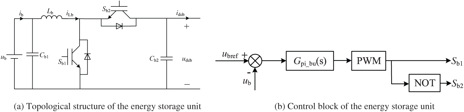
Figure 4: The topology and control structure of energy storage unit

In Fig. 4, ubref is the DC bus voltage reference value, ub is the output voltage of the energy storage converter, and Gpi_bu(s) is the transfer function of the constant voltage controller. The charging or discharging of the energy storage battery is controlled by regulating the on-off states of the switching devices Sb1 and Sb2. Based on the topology of the bidirectional DC-DC converter and the conduction states of the switching devices, small disturbances are introduced around the steady-state operating point of the energy storage converter. By eliminating the steady-state quantities and high-order terms, the linearized small-signal mathematical model of the energy storage converter after analysis is obtained as follows:

{LbdΔiLbdt=Δub−(1−Db)Δudcb+UdcbΔdbCb1dΔubdt=Δib−ΔiLbCb2dΔudcbdt=(1−Db)ΔiLb−ILbΔdb−Δidcb(13)

After Laplace transformation, the small-signal state-space equations in the frequency domain mode can be obtained as follows

{sLbΔiLb=Δub−(1−Db)Δudcb+UdcbΔdbsCb1Δub=Δib−ΔiLbsCb2Δudcb=(1−Db)ΔiLb−ILbΔdb−Δidcb(14)

where Δdb is the duty cycle disturbance value of the energy storage DC-DC converter.

According to the control block diagram of the energy storage converter, the control equation for the small disturbance of the output duty cycle can be obtained as follows:

Δdb=(Δubref−Δub)Gpi_bu(15)

where Gpi_bu = kpb + kib/s is the transfer function of constant voltage for energy storage DC-DC converter.

By combining Eqs. (14) and (15), the DC-side impedance of the bidirectional DC-DC converter in the energy storage unit can be obtained as follows:

Zdcb=−A7(s)sCb2A7(s)+(1−Db)A8(s)(16)

where

A7(s)=s2LbCb1+1−UdcbGpi_bu(s)A8(s)=sCb1(1−Db)+ILbGpi_bu(s)(17)

2.3 Model of the PV Units

PV units typically operate in maximum power point tracking (MPPT) mode to achieve the maximum power output of photovoltaic cells. The photovoltaic power generation unit is connected to the DC bus through a Boost converter. Fig. 5a shows the topological structure of the Boost converter for the PV unit, and the corresponding control block is shown in Fig. 5b.

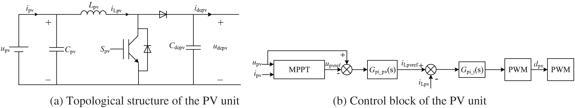
Figure 5: Topology and control block diagram of PV unit

In Fig. 5, the ipv, upv are the output voltage and current for PV. Cpv, Lpv, Cdcpv are respectively the capacitor on the photovoltaic string side, the equivalent inductor of the converter, and the DC-side capacitor. iLpv, idcpv, udcpv are respectively the converter inductor current, the output DC current at the converter port side, and the DC voltage. Spv is the converter switching function.

Based on the topology of the PV unit converter shown in Fig. 5a, impedance modeling is performed for the Boost converter. According to the on-off states of the switching devices, small-disturbance linearization is carried out around the steady-state operating point of the photovoltaic Boost converter. After neglecting the steady-state terms and high-order terms, the small-signal mathematical model under small-disturbance conditions can be obtained as

{LpvdΔiLpvdt=Δupv−(1−Dpv)Δudcpv+UdcpvΔdpvCpvdΔupvdt=Δipv−ΔiLpvCdcpvdΔudcpvdt=(1−Dpv)ΔiLpv−ΔdpvILpv−Δidcpv(18)

where Δdpv is the duty cycle disturbance value of the PV Boost converter.

By performing Laplace transform on Eq. (18), the small-signal mathematical model in the frequency domain mode can be obtained a

{sLpvΔiLpv=Δupv−(1−Dpv)Δudcpv+UdcpvΔdpvsCpvΔupv=Δipv−ΔiLpvsCdcpvΔudcpv=(1−Dpv)ΔiLpv−ΔdpvILpv−Δidcpv(19)

where Dpv is the steady-state value of the duty cycle of the Boost converter, and its specific expression is Dpv = 1 – Upv/Udcpv. Upv is the steady-state value of the photovoltaic cell voltage. Idcpv is the steady-state value of the inductor current of the Boost converter. Udcpv is the steady-state value of the port voltage on the DC bus side. Idcpv is the steady-state value of the DC-side current.

According to the control block diagram of the photovoltaic Boost converter, the duty cycle control equation of the converter under small-signal disturbance is obtained as

Δdpv=Gpi_i(ΔiLpvref−ΔiLpv)=Gipv[(Δupv−Δupvref)Gupv−ΔiLpv](20)

where Gupv = kpv1 + kiv1/s, Gipv = kpv2 + kiv2/s is the transfer function of the outer and inner control loop. By combining Eqs. (19) and (20), the DC-side impedance of the PV unit can be obtained as

Zpv=A5(s)sCdcpvA5(s)+sCpv(1−Dpv)A6(s)(21)

where

A5(s)=s2LpvCpv+sCpvUdcpvGipv+UdcpvGipvGupv+1A6(s)=(1−Dpv)+ILpvGipv+ILpvGipvGupv1sCpv(22)

2.4 Model of the Constant Power Loads

Constant power loads, as the main type of load in DC distribution areas, are considered to be connected to the DC bus via DC-DC converters, with their topological structure and control strategy shown in Fig. 6a,b, respectively.

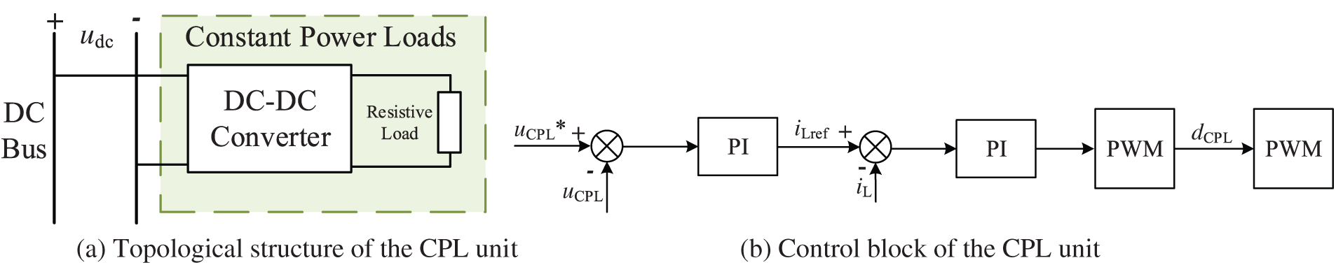
Figure 6: Topology and control block diagram of constant power loads

The voltage and current relationship for a constant power load connected to a DC bus can be expressed as

PCPL=uCPLiCPL(23)

where uCPL is the DC bus voltage, iCPL is the load current of the constant power loads, PCPL is load power.

The impedance modeling of the constant power load is carried out near the steady-state operating point using the small-signal linearization method. The steady-state operating point voltage UCPL serves as the linearization reference point. Through linearization processing based on the first-order Taylor series expansion, the small-signal mathematical model of the constant power load is obtained as follows:

iCPL=PCPLUCPL−PCPLUCPL2(uCPL−UCPL)=2PCPLUCPL−PCPLUCPL2uCPL(24)

Based on Eq. (24), the small-signal impedance model of the constant power load can be obtained as

ZCPL=RCPL=−UCPL2PCPL(25)

3  Impedance Stability Analysis in FIDN System

3.1 Equivalent Impedance Model of FIDN System

In the FIDN system, on the basis of the independent and stable operation of each converter unit, the overall stability of the system is related to the impedance matching characteristics between subsystems. According to the impedance matching theory and system topology analysis, there are dynamic interaction processes in three intervals in the flexibly interconnected distribution network as shown in Fig. 7. AC area I has an interaction between AC distribution Area I and the AC side of converter VSC1. DC Area has an interaction between the DC side of converter VSC1 and the DC side of converter VSC2, and this dynamic interaction process also includes the mutual interaction between the PV unit and the energy storage converter in the DC distribution network. AC Area II has an interaction between the AC side of converter VSC2 and AC distribution area II.

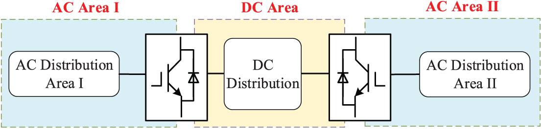
Figure 7: Interactions diagram of FIDN system

Based on the established small-signal model, the equivalent impedance diagram of the DC distribution area interacting with the VSCs on both sides can be obtained. The simplified equivalent circuit diagram of the DC interval impedance can be obtained as Fig. 8. ZVSC1_dc and ZVSC2_dc care respectively the DC-side impedances of converters VSC1 and VSC2. Zpv is the output impedance of the PV unit. Zbat is the output impedance of energy storage unit. Zload is the constant power load, and Zd is the line impedance of DC bus. ZA_out and uA_out are respectively the equivalent impedance and equivalent voltage source on the source side. ZB_in and iB_in are respectively the equivalent impedance and equivalent current source on the load side of the DC interval.

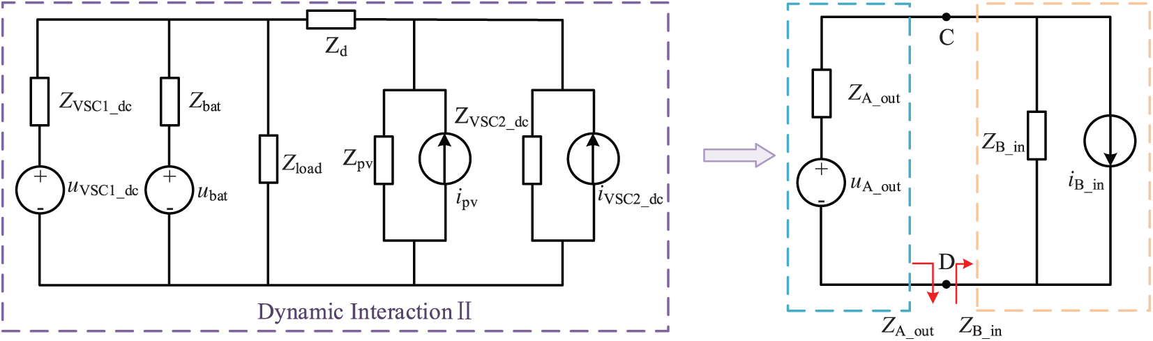
Figure 8: Interval impedance diagram of DC distribution area

From Fig. 8, the total output impedance and total input impedance can be obtained as

ZA_out=ZVSC1_dc//ZpvZB_in=Zbat//((ZVSC2_dc//Zload)+Zd)(26)

3.2 Impedance Characteristics Analysis of FIDN System

Based on the established equivalent circuit model and combined with the parameters in Table 1, the Bode diagrams of the input and output impedances in the DC area can be obtained, as shown in Fig. 9. It can be seen that the total output impedance characteristics of the DC interval are closely related to converter VSC1, and the total input impedance characteristics are related to the constant power load in the DC distribution network area and converter VSC2. The parameters related to the converter’s DC-side impedance model include: the equivalent inductance L on the converter’s AC side, equivalent resistance R, DC-side capacitor Cdc, and converter control loop parameters, etc. In addition, the variation of constant power load and the transmitted power on the AC side will affect the impedance characteristics of the DC interval.

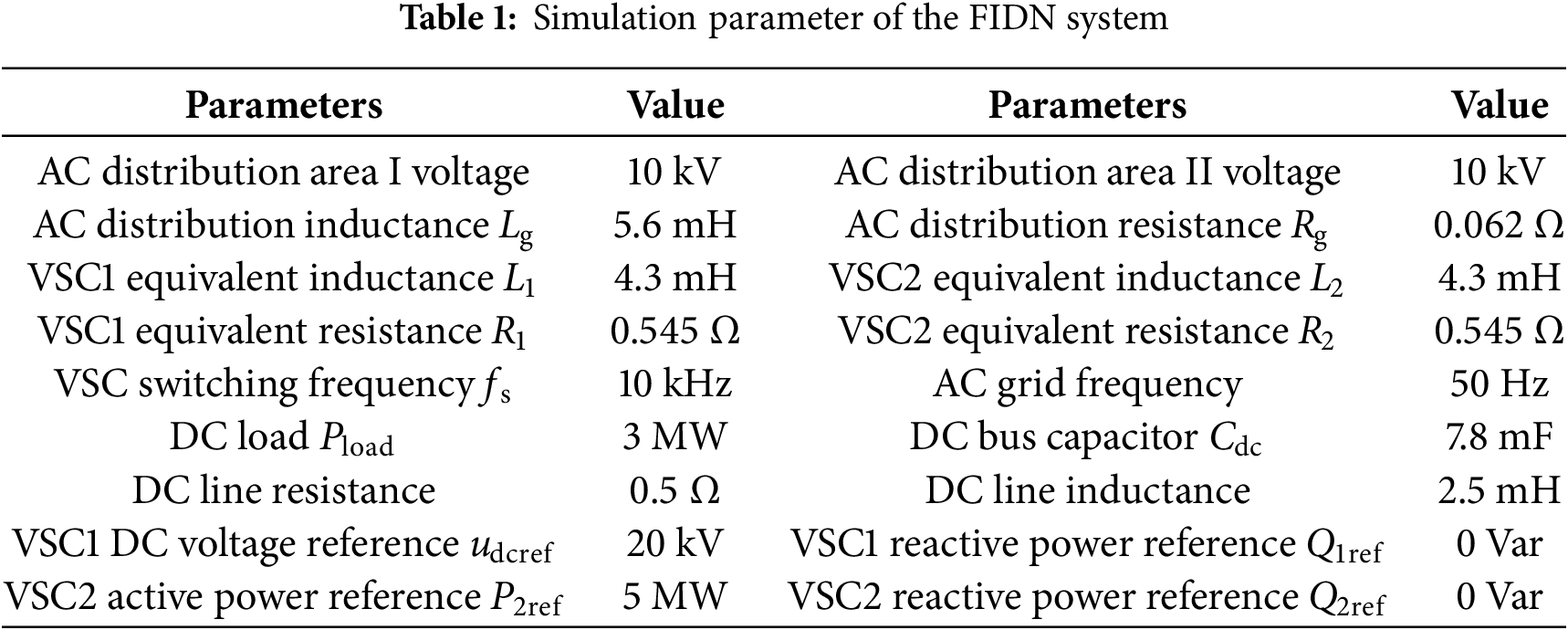
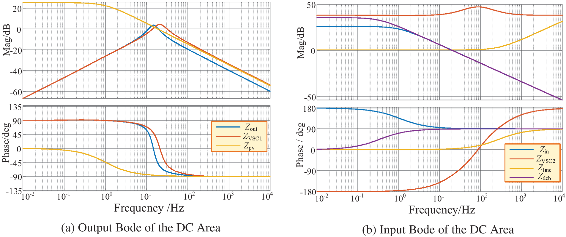
Figure 9: Bode Plot of DC interval output, input impedance

3.3 Analysis of Stability-Influencing Factors

To analyze the impact of AC-side transmitted power on the stability of the FIDN system, Fig. 10a–c, respectively shows the Nyquist curves of the total output/input impedance ratio of the interconnected system under three operating conditions in the DC interval: power transmission direction, different power, and varying constant power load capacities.

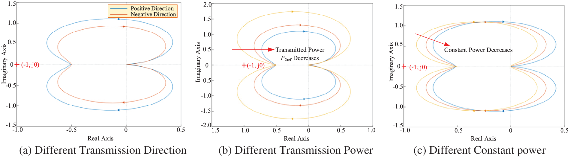
Figure 10: Nyquist curves of DC interval impedance ratio under different operating conditions

It can be seen from Fig. 10a that when power is transmitted in the positive direction, the Nyquist curve of the ratio of total output impedance to input impedance in the DC interval is closer to the (−1, j0) point on the imaginary axis, and the stability margin of the interconnected system is lower than that under the condition of reverse power transmission. As can be observed from the Nyquist curves shown in Fig. 10b,c, when the transmitted power on the AC side is increased or the constant power load is increased, the Nyquist curve of the impedance ratio in the interconnected area continuously approaches the (−1, j0) point, resulting in a decrease in the stability of the interconnected system.

4  Impedance Reshaping Based Stabilization Control

4.1 Control Structures for Impedance Reshaping Based Stabilization Control

To improve the load-carrying capacity of AC feeders and DC lines, this paper proposes a strategy for optimizing active damping control based on impedance reshaping, shown in Fig. 11. By introducing DC voltage feedback, the current inner-loop control of converter VSC1 is optimized to mitigate the DC voltage disturbance caused by load power changes in the interconnected system. Additionally, a DC voltage controller is incorporated into the power outer loop of VSC2, in which the value of the DC voltage controller determines the power variation of VSC2, thereby enabling the tracking of such power changes in VSC2. In which, the GF(s) is the low-pass filter of impedance resharing control in inner current loop of VSC1, and Gdc(s) is the voltage proportional controller of impedance resharing control in outrt active power loop of VSC2, which can be expressed as

GF=kF1+sTGdc=−kdcIdc(27)

where kF is the gain coefficient of the low-pass filter in the voltage feedback loop, and T is the time constant. kdc is the feedback coefficient of the DC voltage stability control, and Idc is the steady-state value of the DC current.

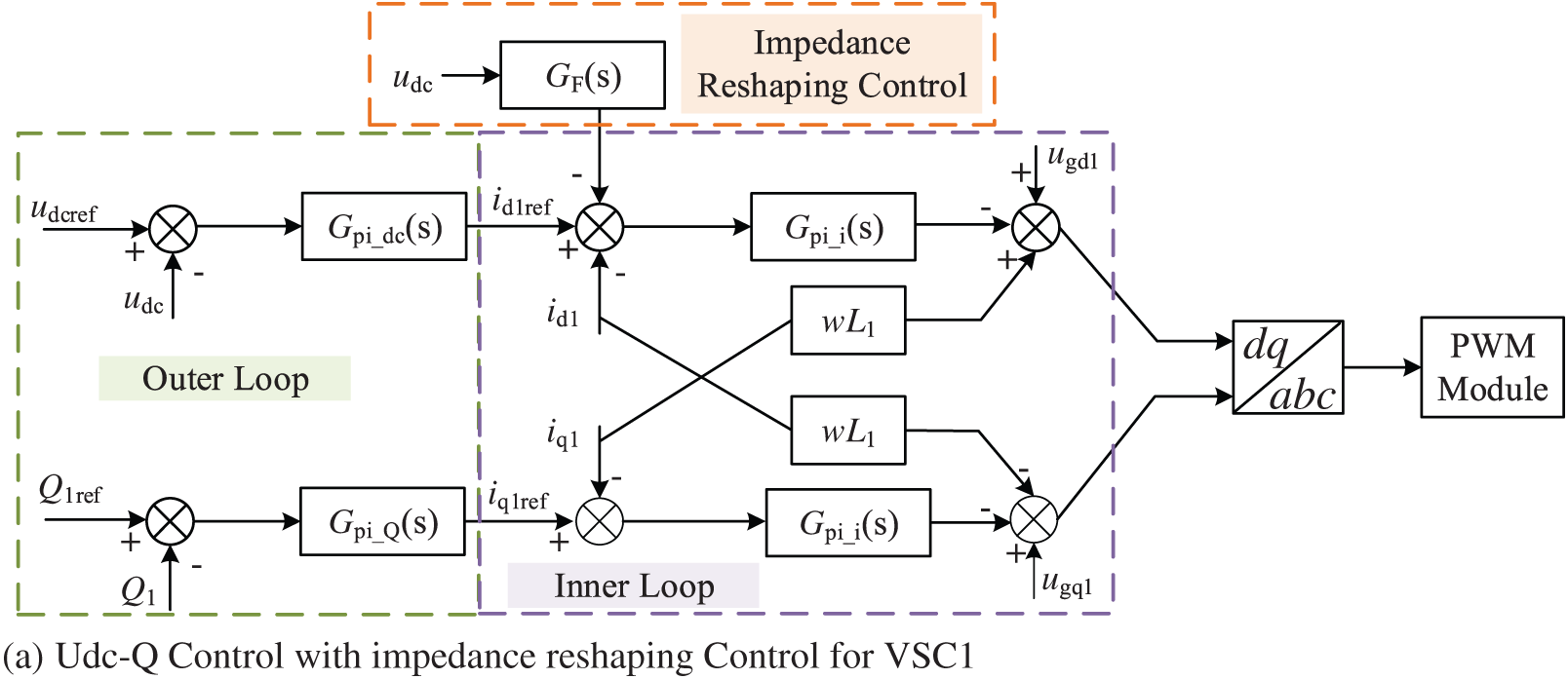
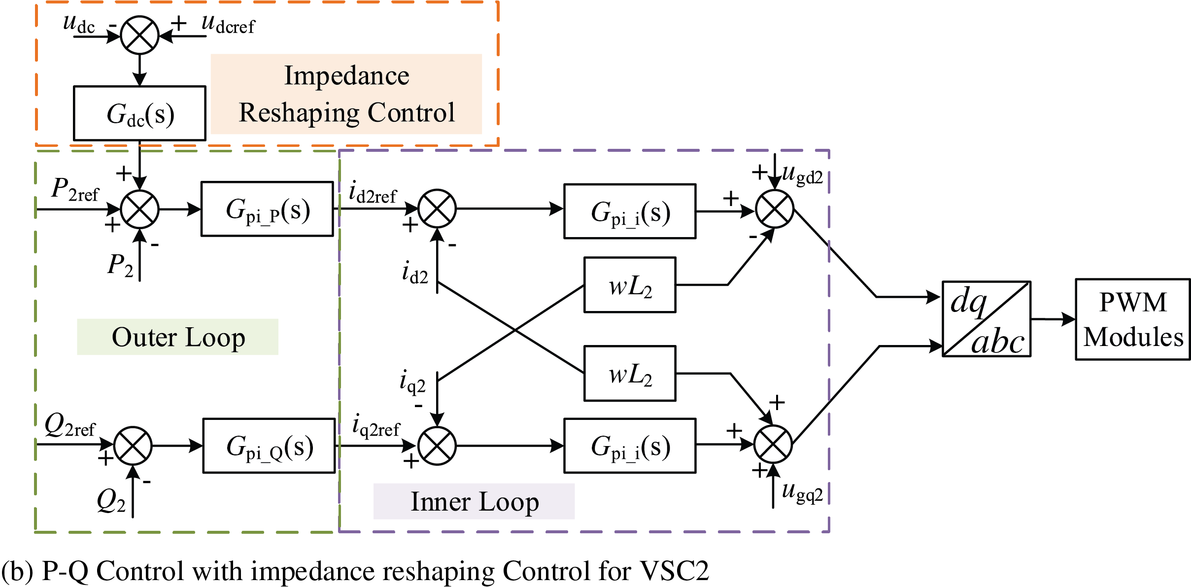
Figure 11: Block diagram of impedance reshaping control strategy for FIDN system

4.2 Stability Analysis for Impedance Reshaping Based Stabilization Control

4.2.1 Small-Signal Impedance Modeling for Impedance Reshaping Based Stabilization Control

(1) Small-Signal Impedance Modeling for VSC1

The proposed control is based on the Eqs. (4)–(6), the small-signal output of the impedance reshaping based stabilization control can be expressed as

{Δdd1Udc=Δugd1+ωL1Δiq1−Gpi_i(Δid1ref−Gpi_FΔudc−Δid1)Δdq1Udc=Δugq1−ωL1Δid1−Gpi_i(Δiq1ref−Δiq1)Δid1ref=(Δudref−Δudc)Gpi_dcΔiq1ref=(ΔQ1ref−ΔQ1)Gpi_Q(28)

After equivalent transformation of Eq. (28), the small-signal output of the control loop can be obtained as

{Δdd1Udc=Δugd1+ωL1Δiq1+Gpi_iΔid1+Gpi_i(Gpi_dc+Gpi_F)ΔudcΔdq1Udc=Δugq1−ωL1Δid1+Gpi_iΔiq1+Gpi_iGpi_QΔQ1(29)

where Gpi_dc, Gpi_Q and Gpi_i are respectively the VSC1 voltage controller, reactive power controller, and current inner-loop controller, GF is the low-pass filter in the DC voltage feedback link of the current inner loop.

Based on Eqs. (28) and (29), the DC-side impedance of converter VSC1 after impedance reshaping can be expressed as

ZVSC1_dc∗=−ΔudcΔidc=UdcB1(s)sCUdcB1(s)+1.5Dd1UdcB2(s)+1.5Id1Gpi_iB2(s)+B3(s)(30)

where B1(s)–B3(s) is

B1(s)=sL1+R1+Gpi_iB2(s)=Dd1+Gpi_i(Gpi_dc+Gpi_F)B3(s)=−1.5Id1Gpi_iB1(s)(Gpi_dc+Gpi_F)(31)

(2) Small-Signal Impedance Modeling for VSC2

Based on the Eqs. (4)–(6), when the impedance reshaping control with a DC voltage feedback link is added to the power outer loop, the small-signal output of the system can be obtained as

{Δdd2Udc=Δugd2−ωL2Δiq2+Gpi_i2(Δid2ref−Δid2)Δdq2Udc=Δugq2+ωL2Δid2+Gpi_i2(Δiq2ref−Δiq2)Δid2ref=(ΔP2ref−ΔP2+(Δudcref−Δudc)Gdc)Gpi_PΔiq2ref=(ΔQ2ref−ΔQ2)Gpi_Q(32)

Further, the small signal output of VSC2 can be obtained as

{Δdd2Udc=Δugd2−ωL2Δiq2−Gpi_i2Gpi_P(ΔP2+GdcΔudc)−Gpi_iΔid2Δdq2Udc=Δugq2+ωL2Δid2−Gpi_i2Gpi_QΔQ2−Gpi_iΔiq2(33)

where Gpi_P, Gpi_Q, Gpi_i2 are respectively the transfer functions of VSC2’s active power control, reactive power control, and current inner-loop controller. Gdc is the controller transfer function of the DC voltage feedback link in the power outer loop.

Based on the Eqs. (32) and (33), when DC voltage feedback is introduced into the outer loop of VSC2, the expression Gui(s) between the d-axis current id2 on the AC side and the DC voltage udc can be expressed as

Gui(s)=Δid2Δudc=Dd2−Gpi_iGpi_PGdc(sL2+R2+Gpi_i(1.5Gpi_PUgd2+1))(34)

The DC-side impedance of converter VSC2 after impedance reshaping can be expressed as

ZVSC2_dc∗=ΔudcΔidc=Udc−Idc2+1.5Ugd2Gui(s)=UdcB4(s)−Idc2B4(s)+1.5Ugd2B5(s)(35)

where B4(s), B5(s) is

B4(s)=sL2+R2+Gpi_i2(1.5Gpi_PUgd2+1)B5(s)=Dd2−Gpi_i2Gpi_PGdc(36)

Fig. 12 plots the comparison of impedance characteristic curves between the total output impedances and total input impedances of the DC power distribution area before and after impedance reshaping. It can be observed that after impedance reshaping, the magnitude peak of the total output impedance in the DC distribution area has been effectively mitigated. Furthermore, with the addition of a voltage control loop in the power outer loop for optimized control, the total input impedance within the frequency band has transitioned from negative impedance to positive impedance. Therefore, the impedance reshaping significantly improves the system’s stability and dynamic response quality by increasing the phase margin, suppressing resonance peaks, and smoothing the phase transition, without weakening the gain robustness. Meanwhile, to validate the effectiveness of the established impedance models, a simulation model of the FIDN system was built in Simulink, and the input and output impedances of the FIDN system were obtained using the frequency sweep method, as shown by the dotted line in Fig. 12. It can be seen that the Bode plot of the established model is basically consistent with the Bode plot obtained by the frequency sweep method, which indicates that the established impedance models can well describe the response of the actual system.

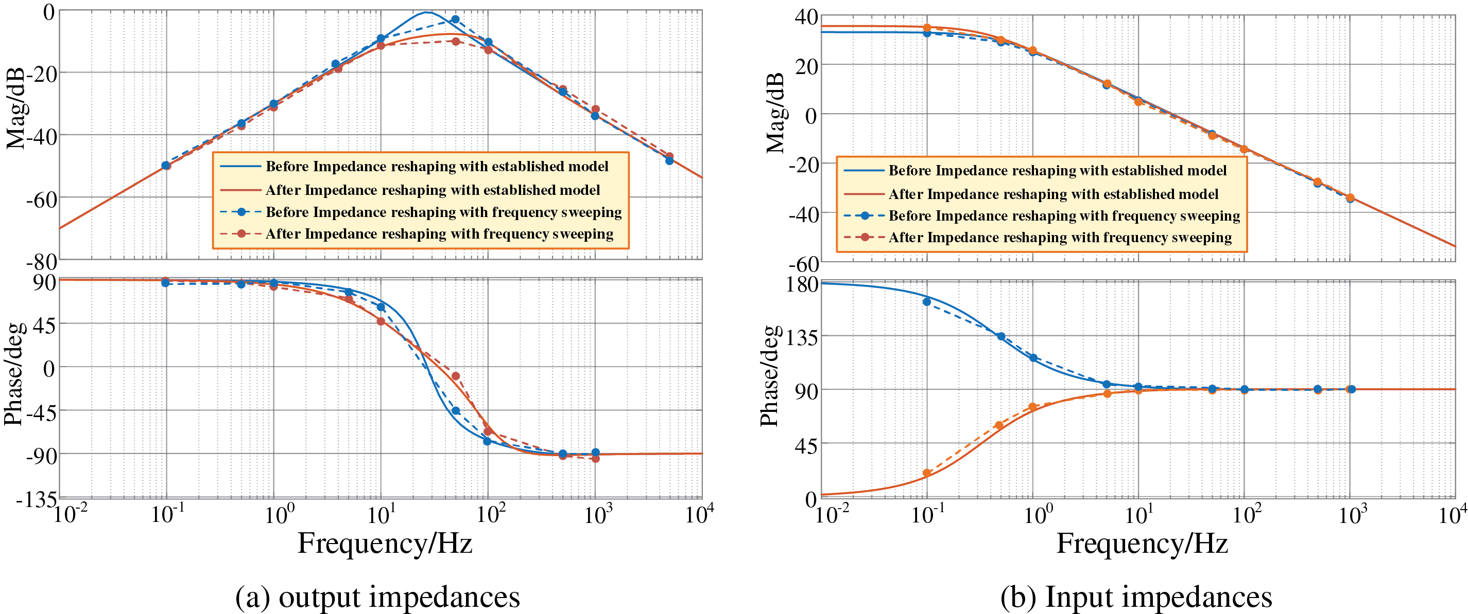
Figure 12: Bode plot of total output and input impedance of DC distribution area before and after impedance remodeling

4.2.2 Stability Analysis for Impedance Reshaping Based Stabilization Control

To tune the values of the gain coefficient of converter VSC1 and the DC voltage feedback coefficient of VSC2, the characteristic curves of total output and total input impedance in the DC distribution network area, and the Nyquist stability analysis via the impedance ratio Tm are compared and analyzed, and the results are shown in Fig. 13. It is determined that the interconnected system achieves good stability when the gain coefficient of the impedance reshaping loop of converter VSC1 is set to kF = 1.5. Regarding the feedback coefficient for the optimized control of the power outer loop of converter VSC2, when this feedback coefficient kdc changes from 2 to 3, the total input impedance exhibits a positive impedance characteristic. Combined with the impedance ratio Nyquist curve, the feedback coefficient is selected as kdc = 5.

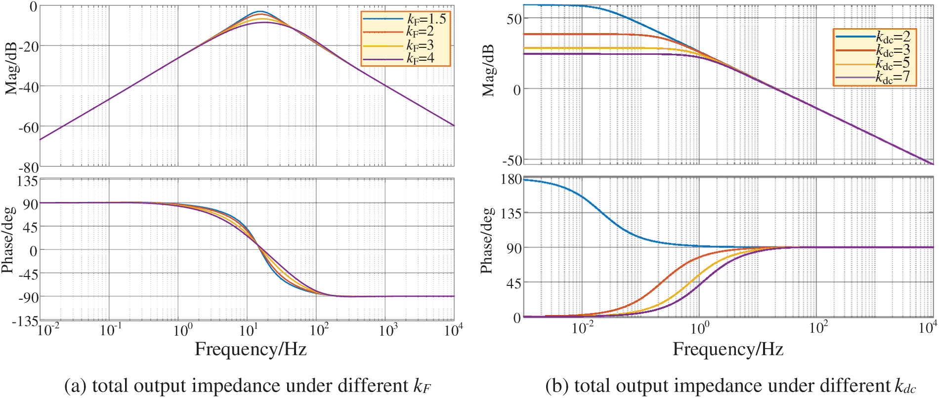
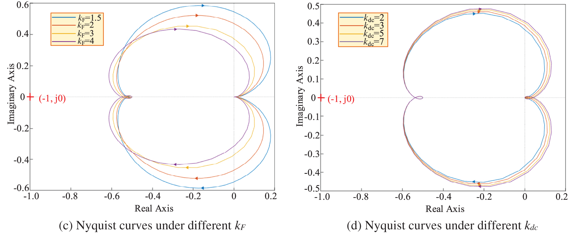
Figure 13: Effect of impedance resharpening coefficient on DC interval impedance

Based on the tuned coefficient, Fig. 14 plots the Nyquist curves comparison of the different consists loads conditions, it can be that Without impedance reshaping, under bidirectional power transmission, the Nyquist curves of the total output-to-input impedance ratio in the DC distribution network area are relatively close to the imaginary axis. However, after impedance reshaping, the area of the Nyquist curves of the output-to-input impedance ratio in the DC distribution network area on the imaginary axis is reduced, resulting in a higher stability margin.

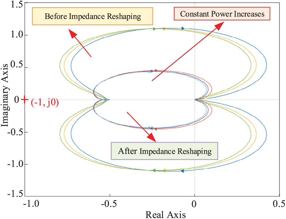
Figure 14: Nyquist curves at constant power load variations before and after impedance reshaping

Fig. 15 plots the Nyquist curves comparison of different power transmission direction, it can be been that without impedance reshaping, under bidirectional power transmission, the Nyquist curves of the total output-to-input impedance ratio in the DC distribution network area are relatively close to the imaginary axis. However, after impedance reshaping, the area of the Nyquist curves of the output-to-input impedance ratio in the DC distribution network area on the imaginary axis is reduced.

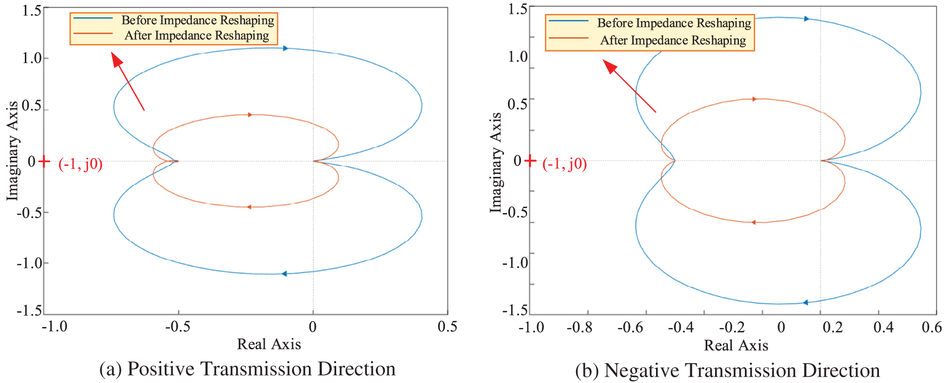
Figure 15: Nyquist Curve for different power transmission direction

5  Simulation Verification

To verify the effectiveness of the proposed stabilization control, an FIDN system as shown in Fig. 1 is built in the Matlab/Simulink simulation software, the simulation parameters are listed in Table 1.

5.1 Power Transmission Variation in the FIDN System

Firstly, set the initial power reference value Pref of VSC2 to 5 MW. During the simulation, set the Pref of VSC2 to 8 MW at 0.5 s, and then regulate it to 10 MW at 1.5 s. The variation of the transmitted power is shown in Fig. 16a. Under this condition, the DC bus voltage waveforms under the conventional control strategy and the proposed impedance reshaping based stabilization control are shown in Fig. 16b,c, respectively. It can be seen that when the magnitude of transmitted power changes, the DC bus voltage is affected, leading to voltage fluctuations. The proposed impedance reshaping control obtains smaller voltage drop and overcharge amplitudes when the system power transmission changes, thus providing better system stability.

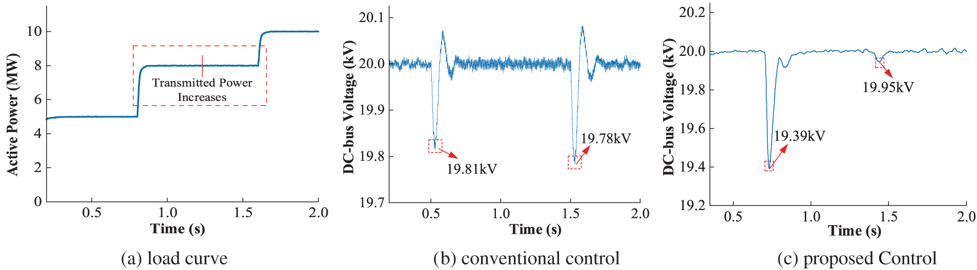
Figure 16: Simulation analysis of transmission power variation in FIDN systems

Secondly, to verify the theoretical research on the stability of the FIDN system under changes in power transmission direction, a simulation verification is conducted by changing the power transmission direction of converter VSC2. The power reference value of converter VSC2 is set to switch to the negative direction at 1.0 s and return to the positive direction at 1.5 s, the variation of the transmitted power is shown in Fig. 17a. Under this condition, the DC bus voltage waveforms under the conventional control strategy and the proposed impedance reshaping based stabilization control are shown in Fig. 17b,c, respectively. It can be seen that the proposed impedance reshaping control obtains smaller voltage drop and overcharge amplitudes when the system power transmission direction variations, thus providing better system stability.

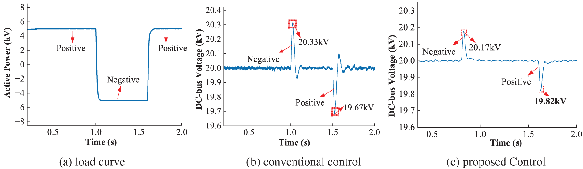
Figure 17: Simulation analysis of transmission direction in FIDN systems

5.2 Constant Load Power Variation in the FIDN System

For the operating condition where the DC distribution network can carry constant power loads, the constant power load is increased from 6 to 12 MW at 0.7 s, and then further increased to 15 MW at 1.4 s. Under different impedance optimization control strategies, the waveforms of DC bus voltage and AC grid current are shown in Fig. 18. Fig. 18b shows the fluctuation curve of DC voltage under constant power fluctuations with the conventional control strategy. It can be seen that when the constant power load changes, the DC bus voltage fluctuates significantly, and there is even a risk of instability at 1.5 s. The proposed control strategy significantly improves the stability of the DC-side voltage through impedance reshaping. Under the condition of constant power load fluctuations, the DC-side voltage can remain stable around the reference value, demonstrating higher system stability.

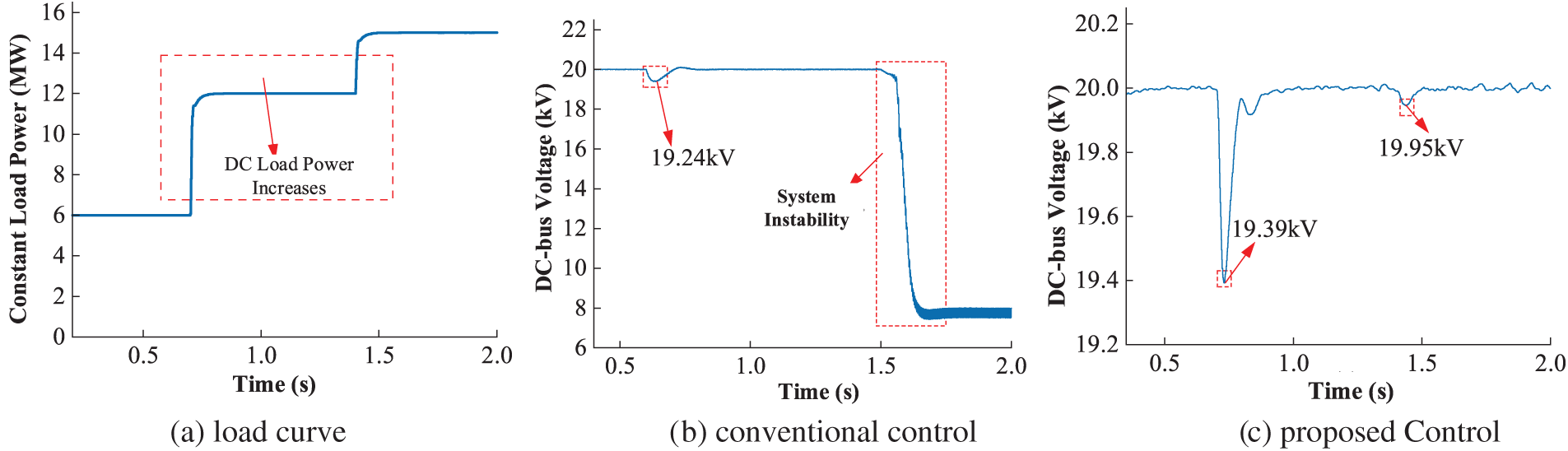
Figure 18: Simulation analysis of different constant load conditions in FIDN systems

5.3 AC Voltage Sags in the FIDN System

To verify the stability enhancement capability of the proposed impedance reshaping based stabilization strategy during AC voltage sags, a comparative analysis was conducted under the voltage sag condition. At the initial moment, the AC grid voltage was in a normal operating state, while the voltage dropped to 0.4 p.u. at 1.0 s. The waveforms of the DC bus voltage and AC grid current are shown in Fig. 19. When the AC grid voltage sagged to 0.4 times its original value, without the impedance reshaping strategy, the AC grid current surged abruptly and the DC voltage dropped to approximately 2 kV, the system could no longer maintain its original stable operating state. In contrast, with the proposed impedance reshaping control strategy, the DC bus voltage recovered to the set value within approximately 0.2 s after the grid voltage sag, and the system maintained a stable operating state.

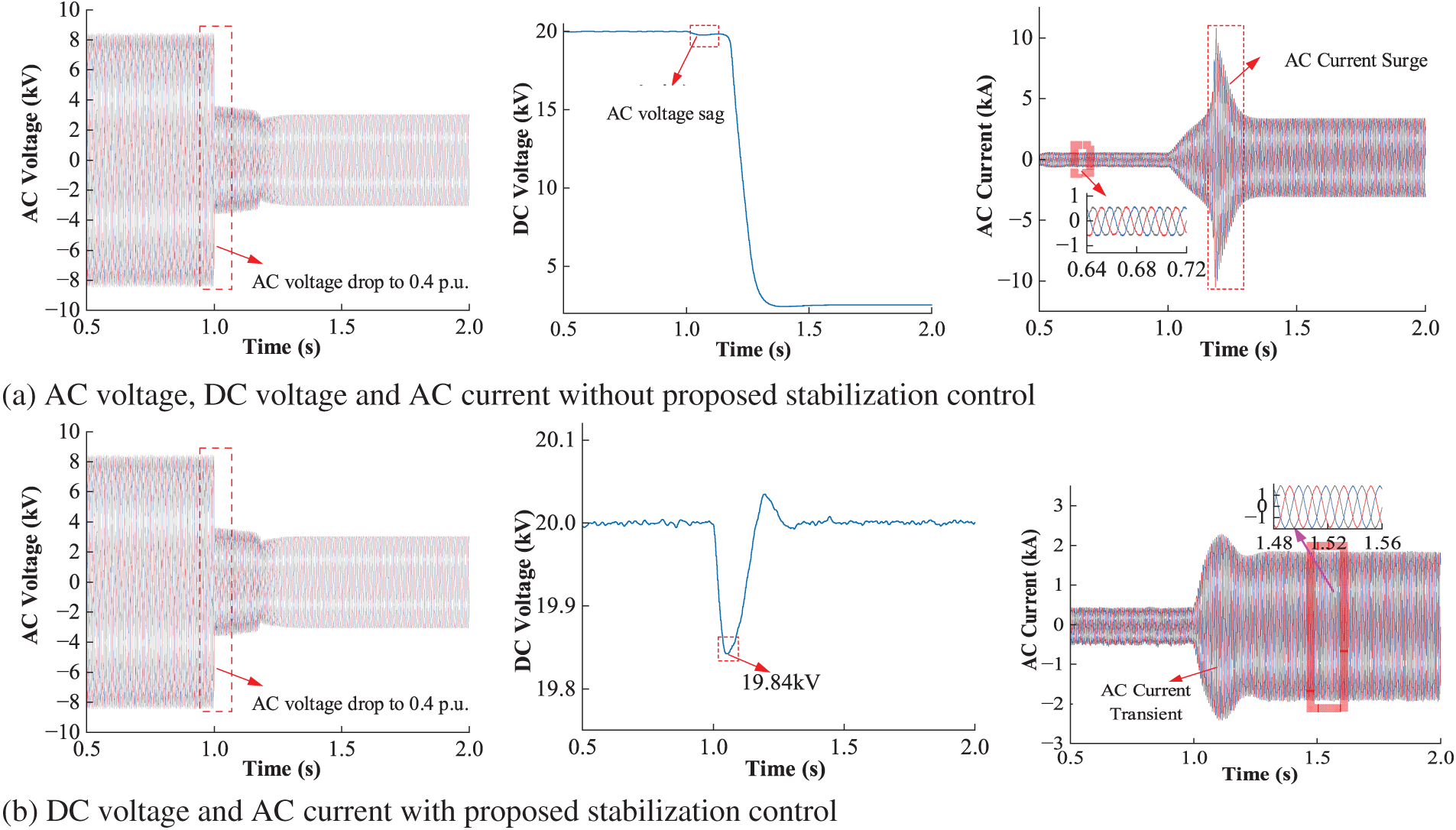
Figure 19: Waveform comparison between the proposed stabilization control and conventional strategy under grid sags conditions

6  Conclusions

This paper proposes an stability analysis and impedance-reshaping-based control strategy to address FIDN stability challenges caused by constant power loads and converter power variations. The key findings are summarized as follows:

(1)   A small-signal impedance model of the converter’s DC side after reshaping quantitatively demonstrates how impedance reshaping mitigates adverse effects of constant power loads and power fluctuations.

(2)   The Nyquist stability analysis verifies that the proposed control improves small-signal stability by reducing the proximity and area of impedance ratio Nyquist curves near the imaginary axis.

(3)   MATLAB/Simulink simulations validate the effectiveness of the proposed method. The results demonstrate that the proposed impedance reshaping strategy effectively mitigates voltage dips, surges, and DC bus fluctuations, shortens transient responses under power variations, and enables rapid stability recovery with reduced voltage drop during severe AC sags.

This work provides theoretical and technical support for stabilizing FIDN systems and ensuring reliable operation. However, the proposed impedance reshaping based stabilization control does not consider the cross-zone impact of output fluctuations of distributed generation (DG) on the AC side on the stability of the DC section. Meanwhile, due to the three-phase three-leg (3P3L) converter cannot provide the zero-sequence current flow path [19,20], which cannot achieve the compensation of three-phase unbalance power. Future research will explore the three-phase four-leg (3P4L) VSC based FIDN system to handle three-phase unbalanced conditions, and cross-zone impact of distributed generation fluctuations on DC stability and the coordinated tuning of impedance control parameters.

Acknowledgement: Not applicable.

Funding Statement: This work was supported by the key technology project of China Southern Power Grid Corporation (GZKJXM20220041), and partly by the National Key Research and Development Plan (2022YFE0205300).

Author Contributions: The authors confirm contribution to the paper as follows: Conceptualization, Yutao Xu; methodology and software, Zukui Tan and Xiaofeng Gu; data curation, Xiaofeng Gu and Zhuang Wu; writing—original draft preparation, Xiaofeng Gu and Jikai Li; writing—review and editing, Qihui Feng; supervision, Jikai Li and Zhukui Tan. All authors reviewed the results and approved the final version of the manuscript.

Availability of Data and Materials: The original contributions presented in the study are included in the article; further inquiries can be directed to the corresponding author.

Ethics Approval: Not applicable.

Conflicts of Interest: The authors declare no conflicts of interest to report regarding the present study.

References

1. Wei YM, Chen K, Kang JN, Chen W, Wang XY, Zhang X. Policy and management of carbon peaking and carbon neutrality: a literature review. Engineering. 2022;8(7):52–63. doi:10.1016/j.eng.2021.12.018. [Google Scholar] [CrossRef]

2. Zhang M, Long Y, Guo S, Xiao Z, Shi T, Xiang X, et al. Stability boundary characterization and power quality improvement for distribution networks. Energies. 2024;17(24):6215. doi:10.3390/en17246215. [Google Scholar] [CrossRef]

3. Kong W, Ma K, Wu Q. Three-phase power imbalance decomposition into systematic imbalance and random imbalance. IEEE Trans Power Syst. 2018;33(3):3001–12. doi:10.1109/TPWRS.2017.2751967. [Google Scholar] [CrossRef]

4. Li G, Li J, Yan K, Bian J. Centralized-distributed scheduling strategy of distribution network based on multi-temporal hierarchical cooperative game. Energy Eng. 2025;122(3):1113–36. doi:10.32604/ee.2025.059558. [Google Scholar] [CrossRef]

5. Guo P, Tian Z, Yuan Z, Qu L, Zhang XY, Zhang XP. Future-proofing city power grids: FID-based efficient interconnection strategies for major load-centred environments. IET Renew Power Gener. 2024;18(15):3003–19. doi:10.1049/rpg2.13027. [Google Scholar] [CrossRef]

6. Guo X, Gan L, Liu Y, Hu W. Coordinated dispatching of flexible AC/DC distribution areas considering uncertainty of source and load. Electr Power Syst Res. 2023;225:109805. doi:10.1016/j.epsr.2023.109805. [Google Scholar] [CrossRef]

7. Fan W, Cao Y, An J, Zhao Z, Tan X, Du J, et al. Research on stability analysis of power router with PV and energy storage based on flexible interconnection. In: 2023 3rd International Conference on Energy Engineering and Power Systems (EEPS); 2023 Jul 28–30; Dali, China. p. 152–8. doi:10.1109/EEPS58791.2023.10256934. [Google Scholar] [CrossRef]

8. Ning X, Ji Y, Shao Y, Yu M, Wu M, Xu Y. Large-disturbance stability analysis of flexible interconnected system of distribution areas considering load-balancing. In: 2023 6th International Conference on Power and Energy Applications (ICPEA); 2023 Nov 24–26; Weihai, China. p. 208–13. doi:10.1109/ICPEA59834.2023.10398624. [Google Scholar] [CrossRef]

9. Zheng Z, Zhang S, Zhang X, Yang B, Yan F, Ge X. Stability analysis and control of DC distribution system with electric vehicles. Energy Eng. 2023;120(3):633–47. doi:10.32604/ee.2022.024081. [Google Scholar] [CrossRef]

10. Zhang Y, Zheng H, Zhang C, Yuan X, Xiong W, Cai Y. T-S fuzzy model based large-signal stability analysis of DC microgrid with various loads. IEEE Access. 2023;11:88087–98. doi:10.1109/access.2023.3305526. [Google Scholar] [CrossRef]

11. Cai Y, Wang Y, Zheng H, Xu Y, He M, Wen X. Large disturbance stability analysis of DC microgrid with constant power load based on sum of square programming estimating attraction domain. In: 2024 7th International Conference on Energy, Electrical and Power Engineering (CEEPE); 2024 Apr 26–28; Yangzhou, China. p. 1194–9. doi:10.1109/CEEPE62022.2024.10586581. [Google Scholar] [CrossRef]

12. Wen B, Boroyevich D, Burgos R, Mattavelli P, Shen Z. Analysis of D-Q small-signal impedance of grid-tied inverters. IEEE Trans Power Electron. 2016;31(1):675–87. doi:10.1109/TPEL.2015.2398192. [Google Scholar] [CrossRef]

13. Khaligh A. Realization of parasitics in stability of DC-DC converters loaded by constant power loads in advanced multiconverter automotive systems. IEEE Trans Ind Electron. 2008;55(6):2295–305. doi:10.1109/TIE.2008.918395. [Google Scholar] [CrossRef]

14. Karimipour D, Salmasi FR. Stability analysis of AC microgrids with constant power loads based on popov’s absolute stability criterion. IEEE Trans Circuits Syst II Express Briefs. 2015;62(7):696–700. doi:10.1109/TCSII.2015.2406353. [Google Scholar] [CrossRef]

15. Cai Y, Xu Y, Liu T, Zheng H, Wang F, He M. Collaborative transfer operation strategy for flexible interconnected systems considering transient stability. In: 2024 IEEE 5th International Conference on Advanced Electrical and Energy Systems (AEES); 2024 Nov 29–Dec 1; Lanzhou, China. p. 319–24. doi:10.1109/AEES63781.2024.10872562. [Google Scholar] [CrossRef]

16. Geng Y, Song X, Zhang X, Yang K, Liu H. Stability analysis and key parameters design for grid-connected current-source inverter with capacitor-voltage feedback active damping. IEEE Trans Power Electron. 2021;36(6):7097–111. doi:10.1109/TPEL.2020.3036187. [Google Scholar] [CrossRef]

17. Zhang X, Ruan X, Tse CK. Impedance-based local stability criterion for DC distributed power systems. IEEE Trans Circuits Syst I Regul Pap. 2015;62(3):916–25. doi:10.1109/TCSI.2014.2373673. [Google Scholar] [CrossRef]

18. Wang J, Dong C, Jin C, Lin P, Wang P. Distributed uniform control for parallel bidirectional interlinking converters for resilient operation of hybrid AC/DC microgrid. IEEE Trans Sustain Energy. 2022;13(1):3–13. doi:10.1109/TSTE.2021.3095085. [Google Scholar] [CrossRef]

19. Aizpuru I, Davila A, Planas E, Cortajarena JA, Martin JL. Phase-independent control of a three-phase four-leg inverter. In: 2023 IEEE 32nd International Symposium on Industrial Electronics (ISIE); 2023 Jun 19–21; Helsinki, Finland. p. 1–6. doi:10.1109/ISIE51358.2023.10228068. [Google Scholar] [CrossRef]

20. Tan Z, Zhou D, Deng S, Li J, Wu Z, Feng Q, et al. Optimum operation of low-voltage AC/DC distribution areas with embedded DC interconnections under three-phase unbalanced compensation conditions. Energy Eng. 2025:1–10. doi:10.32604/ee.2025.069610. [Google Scholar] [CrossRef]