
 Login
Login Register
 Submit a Paper
 Propose a Special lssue
 Open Access
ARTICLE

A New Integrated Numerical Simulation Method for Fracturing-Shut-in-Production of Shale Oil
1 College of Petroleum Engineering, Yangtze University, Wuhan, 430100, China
2 Western Research Institute, Yangtze University, Karamay, 834000, China
3 State Key Laboratory of Low Carbon Catalysis and Carbon Dioxide Utilization (Yangtze University), Wuhan, 430100, China
* Corresponding Author: Guanglong Sheng. Email:
(This article belongs to the Special Issue: Progress and Prospects of Hydraulic Fracture Network Morphology Characterization, Flow Simulation and Optimization Technology for Unconventional Oil and Gas Reservoirs)
Energy Engineering 2026, 123(6), 21 https://doi.org/10.32604/ee.2025.073788
Received 25 September 2025; Accepted 24 November 2025; Issue published 27 May 2026
 View Full Text
 Download PDF
Abstract
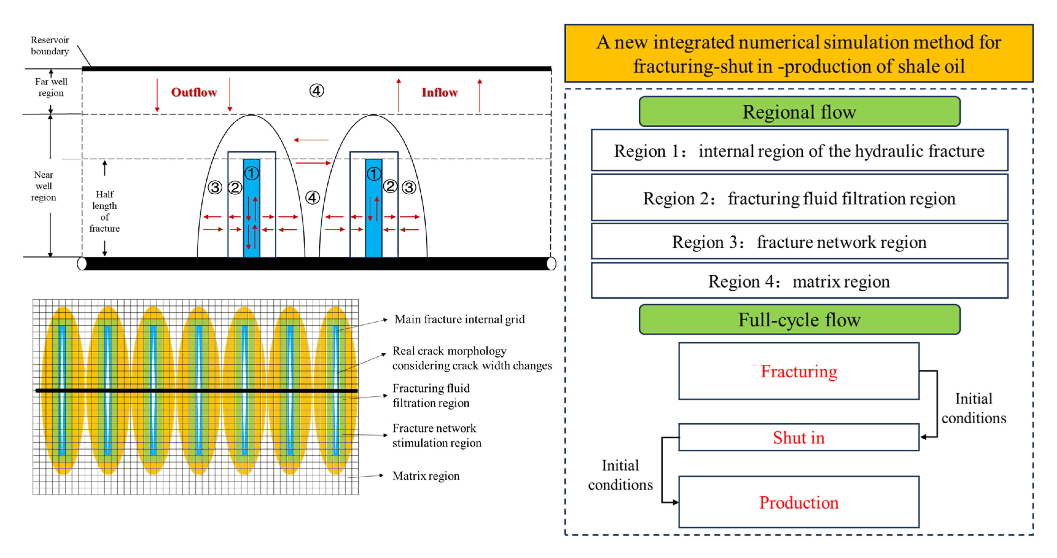
Multi-stage fractured horizontal wells are among the most prevalent technologies in contemporary shale oil development. This article provides a comprehensive overview of several prevalent issues by examining pertinent simulation methods applicable to existing fractured horizontal wells. First, traditional methods primarily concentrate on individual stages of fracturing, shut-in, and production. These stages are relatively isolated and lack continuity. Second, the effects of reservoir stimulation vary under different operational conditions. The conventional dual (or multiple) porosity model is overly idealized, while analytical (or semi-analytical) models often struggle to accurately represent actual fracture geometries and internal fracture-grid characteristics, which limits their ability to effectively describe heterogeneous stimulation effects. In response to these challenges, this paper enhances the single-stage research model employed in traditional approaches by conducting an integrated analysis and establishing a comprehensive flow simulation model that encompasses the entire cycle of fracturing, shut-in, and production stages. Additionally, we introduce the concept of zonal composite flow to partition the reservoir into multiple regions based on specific physical domain partitioning principles; distinct physical property distributions are assigned to each flow region. Furthermore, we improve upon the overall well-fracturing methodology found in traditional techniques by rigorously adhering to actual construction processes. This allows for simulations of common operating conditions such as single-stage fracturing, single multi-stage fracturing events, and pauses in construction between adjacent stages. Finally, utilizing this enhanced method enables us to define evaluation indicators including effective pressure rise ratio (EPER), maximum pressure, and average pressure. We conduct a comparative analysis regarding how factors such as the number of fracturing stages, volume of fracturing fluid injection, and duration of shut-in time influence reservoir energy distribution. The research results show that for the model set up in this article, when the number of fractures is 20, the stimulated regions between fractures exactly overlap, resulting in an EPER of 20.09%, and the best transformation effect is achieved at this time. Additionally, it is determined that the ideal injection volume is 1400 m3 per unit thickness. The most effective duration for well shutdown is identified as 30 days; however, it should be noted that for varying scenarios, the best solution must be derived based on specific operational conditions.Graphic Abstract
Keywords
In the exploitation of shale oil reservoirs, multi-stage fractured horizontal well technology emerges as one of the most widely utilized techniques. This method primarily involves the injection of fracturing fluid at high displacement rates to establish elevated pressure conditions underground, which subsequently generates a complex and extensively distributed network of artificial and induced fractures. This intricate network facilitates the flow of oil within the reservoir through these fractures and into the wellbore, thereby enabling production. The entire process typically encompasses three macroscopic development stages for a horizontal well: fracturing, shut-in, and production.
In the initial phases of research, scholars’ investigations into these developmental stages were relatively fragmented, often concentrating on only a single process. Zhi et al. used numerical simulation to study the inter-seam interference effect and overall transformation effect under different segment cluster ratios [1]. Lu et al. proposed that during the fracturing stage, construction parameters such as fracture spacing and displacement need to be designed according to the sweet spot type [2]. Combining indoor mechanical experiments, Suo et al. confirmed that there are differences in the shape of fractures formed under different in-situ stress conditions, and it is necessary to select fracturing fluids with different properties to obtain the best fracturing effect [3]. Jiang et al. established a transient heat transfer model for multi-stage fracturing of shale oil and gas, and used numerical simulation methods to study the impact of temperature changes on the fracturing effect during the multi-stage hydraulic fracturing process [4]. Zhang et al. established a seepage model coupling fractures and wellbore in shale oil horizontal wells, and proposed a calculation method for the optimal section length of horizontal wells [5]. It is not difficult to find that the research conducted by the above scholars focuses on the impact of various construction parameters on the reservoir stimulation effect in a single fracturing stage. In addition, some scholars have also conducted research on the shut-in stage. Wang et al. built a mechanism model to study the changing trend of shut-in time with crude oil viscosity, bottom hole pressure, matrix permeability, and specific surface area and established a calculation model for the optimal shut-in time [6]. Based on the reservoir pressure distribution and fracture morphology after fracturing, Wang et al. studied the impact of parameters such as displacement, reservoir physical properties, and fracturing fluid performance on the optimal shut-in time [7]. Wijaya and Sheng explored the pros and cons of shut-in after fracturing [8]. Hu et al. established an analytical model of pressure distribution and stimulated volume for shut-in time in shale oil reservoirs, and proposed an optimization method for shut-in time [9]. Zhan et al. established a dynamic geomechanical model to simulate the operating procedures of the fracturing stage based on the expansion morphology of the complex fracture network and the underground fluid seepage mechanism. This study can accurately simulate the formation process of the stimulation zone and the change rules of the reservoir physical properties during the fracturing stage [10]. However, fracturing, shut-in, and production are three continuous physical processes in the development of horizontal wells in shale reservoirs. Establishing a full-cycle simulation study of fracturing, shut-in, and production in shale reservoirs is of great significance for clarifying the interactions between different development stages and formulating corresponding development policies for different stages. At present, domestic and foreign scholars have carried out relevant research on this issue.
Chen et al., focusing on the optimization of fracturing operational parameters, conducted a study on a shale oil reservoir in the Changqing Oilfield [11]. By establishing a numerical model of a multi-stage fractured horizontal well, they developed an integrated method for optimizing fracturing parameters, shut-in time, and well spacing. Xing et al. investigated the functions and properties of different working fluid systems under the conditions of fracturing, shut-in, and flowback, conducting research on the development and improvement of an integrated working fluid [12]. However, much of the related research is approached from an experimental standpoint and focuses primarily on the performance of various working fluids. Li et al. established an integrated simulation model covering the entire life cycle of fracturing, shut-in and production in shale gas reservoirs and completed the state field transfer between different production stages. Eventually, they obtained an optimization method for shut-in time [13]. Based on this, the fracturing and shut-in period was divided into initial fracturing, main fracturing, and early, middle, and late shut-in stages. The study primarily investigated the dual role of shut-in—both promoting and inhibiting—on the subsequent production phase and determined the optimal shut-in time under different conditions. Boronin et al. developed a modeling workflow by coupling the fracturing stage with the post-fracturing flowback and subsequent production phases, revealing the impact of different flowback strategies and operational parameters on the effectiveness of the fracture treatment [14].
Upon a comprehensive analysis of the issues and shortcomings identified in the aforementioned research, the author has discerned several key deficiencies. While these studies consider the three stages of exploitation in an integrated manner, they uniformly adopt a fracturing model wherein multiple stages and clusters initiate simultaneously. This approach fails to simulate sequential fracturing operations that align with actual field procedures, thereby hindering the accurate characterization of fracture interference during the fracturing stage. Moreover, these studies neglect to account for changes in fracture permeability resulting from variations in aperture during both fracture opening and closure; they also overlook the filtration processes occurring during fracturing fluid injection. Additionally, the author asserts that when conducting research on fractured horizontal wells, it is essential to couple wellbore dynamics to accurately calculate pressure gradient distribution. The rationale behind this assertion lies in the fact that modern fractured horizontal wells within shale reservoirs are typically characterized by significant burial depths. When high-rate fracturing fluid is injected through several kilometers of vertical wellbore, it inevitably induces a substantial frictional pressure drop gradient; although drag reducers are commonly employed, this pressure loss remains non-negligible. Particularly in wells with extensive horizontal sections, the pressure drop within the horizontal wellbore is significantly more pronounced than that observed in the vertical section. In such instances, employing an isobaric treatment for perforation locations—a common practice in conventional models—can result in substantial inaccuracies. Therefore, it is imperative to explicitly define the pressure distribution at all points within the wellbore and to conduct a differentiated calculation and characterization of the initial pressure for each perforation point across every cluster and stage. Table 1 illustrates the advantages of the research methodology presented in this paper compared to current mainstream research methods concerning specific issues.

2.1 Model Establishment Process
Based on the characteristics of multi-stage fracture distribution and reservoir stimulation during the volume fracturing of horizontal wells in shale oil reservoirs, this study constructs a two-dimensional unsteady-state flow physical model. This model employs discretized grid cells to partition the reservoir, including its fractures and matrix, into four distinct flow regions: Region 1 refers to the internal area of the hydraulic fracture. Within this region, the flow dynamics of oil and water in two phases are examined. An analytical model that incorporates fracture aperture is used to characterize the variation of grid permeability along the fracture’s propagation direction. Region 2 is designated as the filtration zone for fracturing fluid, depicted in green in the figure. This region accounts for the varying intensity of the filtration effect based on different fracturing fluid properties. It equivalently represents the permeability alteration in the matrix adjacent to the fracture caused by fluid filtration. Region 3 is the fracture network region, shown in yellow. This region is designed to simulate the complex fracture network that forms concurrently with the main hydraulic fracture. Within this region, fractal theory is applied to calculate the permeability variation at different distances from the main fracture. Region 4 is the matrix region. This region is handled using conventional methods and requires no special treatment. It is specifically shown in Figs. 1 and 2.

Figure 1: Staged fracturing model of shale oil reservoirs

Figure 2: Schematic diagram of zoning and fluid flow in shale oil composite flow model
The fundamental assumptions of the model presented in this paper are as follows: (1) The reservoir is defined as a rectangular, box-shaped closed domain with no-flow boundaries. A multi-stage fractured horizontal well is situated at the center of the reservoir, extending across its entire volume. (2) Fractures are positioned symmetrically and uniformly on both sides of the horizontal wellbore. The main hydraulic fractures are assumed to fully penetrate the vertical thickness of the shale oil reservoir. The fractures have finite conductivity, and oil-water two-phase flow is considered within these main fractures. (3) During the production process from the shale oil reservoir, changes in reservoir temperature are not considered (isothermal conditions). The effects of gravity and inertial forces are neglected. Both the rock and the fluids are assumed to be slightly compressible. (4) The fracture and matrix grids adhere to the regional partitioning described above, and the permeability of each distinct region is calculated using a differentiated method. (5) The horizontal well is completed as either an open hole or a cased hole with perforations. Production is maintained at a constant bottom-hole flowing pressure. The pressure at each perforation point is treated differentially, with values obtained from multiphase flow calculations within the wellbore.
Based on these assumptions, the flow of any phase p (water or oil) in the two-phase system is described by:
Applying Darcy’s law to the second term of Eq. (1) and neglecting gravity and capillary forces, the term becomes:
For a slightly compressible fluid,
Therefore, the flow equations of the water and the oil can be expanded as:
In the above formula:
Formula (5) can be rewritten as:
The preceding equation serves as the general model for oil-water two-phase flow in the various regions, where
Region 1: In the fracture region, the solution is obtained using an analytical KGD model that considers variable fracture aperture. This approach is based on the following classic KGD model assumptions: (1) The rock formation obeys the principles of linear elasticity. (2) The fracture height is assumed to be constant. (3) The fracture has an elliptical cross-section, with the maximum width at the center and sharp, cusp-like tips at its ends. (4) The fracturing fluid is a Newtonian fluid.
With the aforementioned assumptions, the analytical solution for the fracture aperture,
In the above formula:
The permeability of any grid block along the fracture path is determined by the fracture aperture according to the following equation:
After the merger, it can be simplified:
In this equation,
Region 2: Traditional filtration theory defines three factors that influence fracturing fluid filtration: (1) the viscosity of the fracturing fluid, (2) the compressibility of the rock and the fluid, (3) the wall building properties of the fluid. Fracturing fluids typically contain chemical additives, such as thickeners, which form a filter cake on the fracture face during the filtration process. This filter cake causes the filtration rate to be non-constant, continuously decreasing over time. Currently, there is no suitable analytical model to calculate this dynamic filtration rate. Therefore, it is necessary to measure the time-dependent filtration rate of the fracturing fluid in rock cores through laboratory experiments. The variation in the filtration rate is then quantitatively characterized by two parameters: the filtration coefficient and the time exponent. As the filtration rate changes, the fluid flow capacity of the filtration region changes concurrently. Consequently, a time-dependent permeability model for the filtration region is constructed to correspond with the time-varying filtration rate.
From the aforementioned formula, we can derive the temporal variation of permeability within the filtration region as follows:
In this formula,
In the initial stage of fracturing fluid injection, when the filtration time is short, the filter cake has not yet fully formed. At this stage, the permeability of the filtration region can be assumed to be equal to that of the external matrix region:
In this formula,
Region 3: External to the main fracture and the filtration region, an elliptical region is established to enclose the fracture system. This region serves to equivalently represent the secondary fractures that are generated along with the main fracture. Within this region, the permeability variation is quantitatively calculated using the fractal dimension of the secondary fracture spacing and the fractal dimension of the secondary fracture aperture [15,16]. The specific calculation method is as follows:
In this formula,
In addition, region 4 is the outermost matrix region, and the permeability of this part of the grid is not treated and is denoted as
The preceding section introduced the model construction and solution approach for a multi-stage fractured horizontal well in shale oil during the fracturing period. Building upon this procedure, this paper now constructs the flow simulation models for the subsequent shut in and production stages.
In handling this problem, the division of flow regions for the shut in and production stages is the same as that set in Section 2.1. A four-level flow region division is similarly used for the solution. Therefore, the governing flow equations for the three stages—fracturing, shut-in, and production—can be written as:
In this formula:
In the above equation, the subscript N for parameters such as pressure and permeability represents the four flow regions. The subscript m denotes the development period, where 1, 2, and 3 correspond to the fracturing, shut-in, and production periods, respectively. The finite difference method is applied to discretize these equations. The resulting system of difference equations is solved using the IMPES method, in which pressure is solved for implicitly and saturation is solved for explicitly. This ultimately yields the pressure and saturation for any grid block at any time. Subsequently, the production rate for each phase is calculated by combining these results with parameters such as oil and water mobility. Assuming a closed outer boundary and a virtual grid, then:
When using the constant pressure calculation mode, the injection volume at different fracture locations is:
Among them,
This article finalizes the equation-solving process in MATLAB and develops a corresponding solving simulator. The comprehensive construction and solution methodology of the model is illustrated in Fig. 3.

Figure 3: Overall construction and solution process of the model
3 Analysis of Influencing Factors
To investigate the impact of fracture quantity on the post-fracturing energy distribution within the reservoir, this study employed eight model cases with fracture counts set at 5, 10, 15, 20, 25, 30, 35, and 40. All other parameters were maintained constant throughout the analysis. It is important to note that this study assumes a uniform distribution of fractures across the reservoir; consequently, as the number of fractures increases for a fixed reservoir size, the spacing between segments decreases. In the predefined reservoir model measuring 4000 m2 × 2000 m2, increasing the number of fractures from 5 to 40 resulted in a reduction of fracture spacing from 750 to 90 m. The relevant parameter settings for each model are presented in Table 2, while Table 3 illustrates the corresponding relationship between fracture quantity and spacing.


Building on this foundation, it is assumed that the Stimulated Reservoir Volume surrounding each fracture has a fixed size and does not vary with the segment spacing. Consequently, as the segment spacing decreases, the SRV region between adjacent fractures will gradually approach each other until they overlap. The specific spatial distribution is illustrated in the figure below.
In the SRV distribution diagrams for different fracture counts shown in Fig. 4a–h, the red line fractures represent fractures uniformly distributed in a reservoir model of the same scale. The purple elliptical region around each fracture is its Stimulated Reservoir Volume (SRV). In this model, with a fracture half-length of 150 m, the elliptical SRV is assumed to have a semi-major axis of 170 m (along the fracture direction) and a semi-minor axis of 100 m (perpendicular to the fracture direction), resulting in a single-fracture SRV region of 53,407 m2. As can be seen from the figures, when the number of fractures is less than 20, the SRV of each fracture remains independent. When the number of fractures reaches 20, the fracture spacing is 200 m, and the SRV regions of adjacent fractures become exactly tangent. As the fracture count continues to increase, the SRVs from different fractures begin to overlap, and the degree of this overlap becomes increasingly severe. Logically, this has two consequences. First, the overlap of stimulated regions leads to intensified stress interference between fractures, which reduces the effective stimulated volume of a single fracture. Second, fluid flow within the overlapping regions may cause localized, ineffective circulation, thereby impacting the uniform distribution of the fracturing fluid and the overall effectiveness of the treatment. This, in turn, can reduce the overall stimulation effectiveness of the reservoir. We will now further analyze this issue using the simulation results from these eight model cases.

Figure 4: Distribution of different fracture numbers. (a) Distribution Map of fracture Network Renovation region (5 fractures); (b) Distribution Map of fracture Network Renovation region (10 fractures); (c) Distribution Map of fracture Network Renovation region (15 fractures); (d) Distribution Map of fracture Network Renovation region (20 fractures); (e) Distribution Map of fracture Network Renovation region (25 fractures); (f) Distribution Map of fracture Network Renovation region (30 fractures); (g) Distribution Map of fracture Network Renovation region (35 fractures); (h) Distribution Map of fracture Network Renovation region (40 fractures)
First, the Fig. 5a–h shows the post-fracturing pressure distribution fields in the reservoir for different numbers of fractures, with each fracture being fractured for 2 h.

Figure 5: The corresponding pressure distribution of different number of fractures. (a) Reservoir pressure distribution after fracturing (5 fractures); (b) Reservoir pressure distribution after fracturing (10 fractures); (c) Reservoir pressure distribution after fracturing (15 fractures); (d) Reservoir pressure distribution after fracturing (20 fractures); (e) Reservoir pressure distribution after fracturing (25 fractures); (f) Reservoir pressure distribution after fracturing (30 fractures); (g) Reservoir pressure distribution after fracturing (35 fractures); (h) Reservoir pressure distribution after fracturing (40 fractures)
To compare and analyze the reservoir pressure changes across the eight scenarios, three metrics were statistically compiled for each case: the Effective Pressure Elevation Ratio (EPER, the proportion of grids where the pressure exceeds 10% of the initial pressure), the average post-fracturing reservoir pressure, and the maximum post-fracturing reservoir pressure. The specific statistical data are presented in the Table 4.

As shown in Figs. 6 and 7, as the number of fracturing fractures increases, EPER of the stimulated reservoir volume exhibits distinct phased characteristics. It is evident that in this model, when the number of fractures is less than 20 (fracture spacing > 200 m), the elliptical stimulated regions of each fracture are independent. In this phase, EPER shows an approximately linear increase with the number of fractures, with the EPER increment fluctuating around 5% for every additional 5 fractures, indicating that new fractures are highly efficient in developing unstimulated parts of the reservoir. When the number of fractures reaches 20, the spacing is equal to twice the semi-minor axis of the elliptical SRV, causing adjacent SRVs to be perfectly tangent. This forms the most compact, non-overlapping arrangement. At this point, EPER reaches 20.09%, and the contribution ratio per fracture peaks at 1.005%, signifying optimal utilization of the stimulated space.

Figure 6: EPER changes with the number of fractures

Figure 7: Reservoir pressure changes with the number of fractures
However, as the number of fractures continues to increase, the SRV begin to overlap, and the growth rate of EPER slows down significantly, approaching a plateau. Specifically, at 25 fractures, the EPER growth rate drops to only about 1% for every 5 additional fractures. This trend confirms the earlier hypothesis: the intensified inter-fracture stress interference caused by SRV overlap leads to a reduction in the effective stimulated volume per fracture, creating large regions of re-fracturing and ineffective fluid circulation. Furthermore, preferential fluid channeling causes the fracturing fluid to flow along already stimulated, high-permeability regions, reducing its contact with new regions and thus worsening the overall pressure elevation effect. A quantitative analysis shows that when the fracture spacing decreases from 200 to 160 m, the overlap ratio reaches 20%, and the EPER growth rate decreases by approximately 18%. When the spacing is further reduced to 90 m, the overlap ratio exceeds 55%, and the EPER growth becomes negligible. Therefore, from an engineering and economic perspective, one should not blindly pursue a higher number of fractures when designing a fracturing operation. Instead, a comprehensive analysis incorporating the SRV of each fracture is required to ensure that the SRVs of individual fractures do not intersect or overlap. This condition not only yields the highest stimulation efficiency but also achieves the optimal economic outcome.
In field fracturing operations, to effectively break down the formation and create fractures, the injection rate is typically high, generally reaching levels of 15–20 m3/min. The fracturing time for a single stage is usually 1–2 h, which means the cumulative injection volume per stage typically reaches 1000–2500 m3. Assuming a cumulative injection of 2000 m3 per stage, and based on the 20 fractures scale set in this paper’s model, the total well injection volume is 40,000 m3. With an assumed reservoir thickness of 40 m, the injection volume per unit thickness for the entire well is 1000 m3. Therefore, this section sets this injection volume as the intermediate value. Ten simulation cases were designed with total well injection volumes per unit thickness of 200, 400, 600, 800, 1000, 1200, 1400, 1600, 1800, and 2000 m3/m. These simulations were conducted to study the impact of different injection volumes on reservoir energy distribution. Fig. 8a–j shows the pressure distribution under different injection volumes. The specific pressure data are shown in Table 5.


Figure 8: The corresponding pressure distribution of different injection volume. (a) Reservoir pressure distribution after fracturing (200 m3); (b) Reservoir pressure distribution after fracturing (400 m3); (c) Reservoir pressure distribution after fracturing (600 m3); (d) Reservoir pressure distribution after fracturing (800 m3); (e) Reservoir pressure distribution after fracturing (1000 m3); (f) Reservoir pressure distribution after fracturing (1200 m3); (g) Reservoir pressure distribution after fracturing (1400 m3); (h) Reservoir pressure distribution after fracturing (1600 m3); (i) Reservoir pressure distribution after fracturing (1800 m3); (j) Reservoir pressure distribution after fracturing (2000 m3)

As shown in Figs. 9 and 10, as the total well injection volume during the fracturing stage increases, the reservoir’s Effective Pressure Elevation Ratio (EPER) and post-fracturing pressure response exhibit distinct phased characteristics. All three metrics—EPER, average post-fracturing reservoir pressure, and maximum post-fracturing reservoir pressure—show an upward trend with increasing injection volume, but their rates of increase and marginal contributions differ significantly.

Figure 9: EPER changes with injection volume

Figure 10: Reservoir pressure changes with injection volume
A comparison of the stimulation response data under different injection volumes shows that in this model, as the total injection volume per unit thickness increases from 200 to 2000 m3, EPER rises from 9.17% to 25.80%, an increase of 16.63%. However, its growth rate is non-linear. At lower injection volumes, EPER grows rapidly, and the stimulation effect is significant. But when the injection volume exceeds 1000 m3, the growth of EPER gradually slows down, ultimately increasing by only 1.21% in the 1800–2000 m3 interval. This trend indicates that as the injection volume continues to increase, the original, unstimulated regions of the reservoir are progressively affected by pressure, and the stimulated fracture network regions tend to overlap. Additional injected volume mainly enters the already-stimulated regions, leading to limited growth in effective stimulated volume and causing a phenomenon of redundant injection, which in turn reduces the overall efficiency of reservoir pressure elevation.
Furthermore, the responses of the average and maximum reservoir pressures follow different patterns compared to EPER. As the injection volume increases from 200 to 2000 m3, the average pressure only rises from 20.51 to 24.17 MPa, a cumulative increase of 3.66 MPa, representing an overall increase of less than 18%. The growth trend is relatively stable. This suggests that the average pressure is more reflective of the overall energy level of the reservoir. Especially when the reservoir is large and the number of wells is small, large far-field regions cannot be effectively reached by the pressure wave. The main pressure increase is concentrated in the near-wellbore region, resulting in a weak correlation between average pressure and injection intensity. In contrast, the response of the maximum pressure is more sensitive. During the increase in injection volume from 200 to 2000 m3, its value rapidly rises from 52.93 to 84.55 MPa, a cumulative increase of over 30 MPa. The main growth phase for the maximum pressure is concentrated in the 600–1200 m3 injection interval, after which it continues to grow but at a significantly slower rate.
Integrating the characteristics of the EPER and reservoir pressure response metrics, it can be concluded that moderately increasing the injection volume is beneficial for expanding the reach of the fracturing fluid and improving the overall reservoir stimulation efficiency. However, once the injection volume exceeds a certain threshold (approximately 1400 m3 in this model), the reservoir transformable space tends to saturate, and the newly injected liquid flows to the modified region, and the effect of unit injection amount on EPER and pressure increase is significantly reduced. At the same time, excessively high injection volumes may also induce adverse consequences such as uncontrolled local fracture propagation, intensified inter-fracture interference, fracturing fluid flowback, and formation damage.
In the development of shale oil reservoirs via hydraulic fracturing, the shut-in period is a critical step that bridges the fracturing operation and the start of production. The duration of this period directly influences the redistribution of the pressure field within the reservoir. By studying the dynamic evolution of pressure under various shut-in durations, the shut-in strategy can be optimized to enhance the effectiveness of the fracturing treatment.
Therefore, this study simulates ten cases with different shut-in durations: 10, 20, 30, 40, 50, 60, 70, 80, 90, and 100 days. For each case, the reservoir EPER, average pressure, and maximum pressure were recorded to analyze the pressure diffusion within the reservoir as a function of shut-in time.
Fig. 11 illustrates the variations in reservoir pressure under different shut-in durations. An analysis of Table 6 indicates that the influence of shut-in time on reservoir pressure distribution exhibits a clear and systematic pattern. As the duration of shut-in is extended, the Enhanced Production Efficiency Ratio (EPER) consistently increases from 21.78% at 10 days to 26.86% at 100 days, resulting in an overall increase of 5.08%. However, it is noteworthy that the growth rate demonstrates a distinct downward trend. Specifically, the most significant increase in EPER occurs within the first 30 days; thereafter, the incremental gain for each subsequent ten-day period gradually diminishes, with only a marginal increase of 0.35% observed between days 90 and 100. This suggests that as shut-in time extends, the extent of pressure diffusion progressively decreases. The specific trend of these changes is depicted in Fig. 12.

Figure 11: The corresponding pressure distribution of different shut-in time. (a) Reservoir pressure distribution after fracturing (10 d); (b) Reservoir pressure distribution after fracturing (20 d); (c) Reservoir pressure distribution after fracturing (30 d); (d) Reservoir pressure distribution after fracturing (40 d); (e) Reservoir pressure distribution after fracturing (50 d); (f) Reservoir pressure distribution after fracturing (60 d); (g) Reservoir pressure distribution after fracturing (70 d); (h) Reservoir pressure distribution after fracturing (80 d); (i) Reservoir pressure distribution after fracturing (90 d); (j) Reservoir pressure distribution after fracturing (100 d)


Figure 12: EPER changes with shut-in time
The variation in maximum pressure is notably significant, exhibiting a continuous decline from 43.97 MPa at 10 days to 33.63 MPa at 100 days, representing a reduction of 23.5%. An analysis of the decline pattern reveals that during the initial 30 days, the cumulative pressure drop amounted to 6.84 MPa, which constitutes 62.3% of the total decrease. The rate of decline slows between days 30 and 60, entering a phase of stable reduction and tending towards stabilization after day 60, ultimately remaining within the range of 33.6–34.2 MPa. The specific trend in these changes is illustrated in Fig. 13. This observation suggests that the reservoir pressure system has effectively achieved dynamic equilibrium. From an engineering application standpoint, it is advisable to avoid excessively prolonged shut-in periods to prevent ineffective waiting and resource wastage.

Figure 13: Reservoir pressure changes with shut-in time
(1) This paper enhances the conventional simulation approach for simultaneous multi-fracture treatments in horizontal wells targeting shale oil. By incorporating inter-fracture interference, a sequential multi-stage fracturing model has been developed, aligning more closely with actual operational practices.
(2) A graded flow model for a multi-stage fractured horizontal well in shale oil has been developed. The grid utilized within the fractures employs the analytical solution for fracture aperture derived from the KGD model, and concurrently calculates the corresponding permeability associated with that aperture.
(3) The matrix region surrounding the fractures is segmented into several distinct regions: a filtration region that accounts for varying filtration velocities, a stimulated reservoir volume (SRV) derived from fractal theory, and a conventional matrix region. The permeability in each of these regions is calculated independently.
(4) To characterize the reservoir energy distribution, the Effective Pressure Elevation Ratio (EPER) for post-fracturing was proposed. Combined with average and maximum reservoir pressure, it serves as an evaluation metric for fracturing effectiveness. The influence of the number of fractures, injection volume, and shut-in time on reservoir energy distribution at different phases was investigated, and the main controlling factors were identified. The results show that there are ascending thresholds for the influence of different factors on pressure increase. For the model set up in this article, with 20 fractures, the stimulated regions overlap perfectly, yielding an EPER of 20.09% and achieving optimal transformation effects. The ideal injection volume is determined to be 1400 m3 per unit thickness. The most effective well shutdown duration is identified as 30 days. However, the best solution for different scenarios must be based on specific operational conditions.
Acknowledgement: Not applicable.
Funding Statement: This work was supported by National Natural Science Foundation of China (Grant No. 52474029), National Natural Science Foundation for Young Scientists of China (A) (Grant No. 52525403), National Major Science and Technology Projects under the 14th Five-Year Plan (Grant No. 2024ZD1405105), Science and Technology Innovation Team Project of Xinjiang Uygur Autonomous Region (Grant No. 2024TSYCTD0018), Xinjiang Uygur Autonomous Region.
Author Contributions: The authors confirm contribution to the paper as follows: Related background research, Hui Zhao; Data collection, Guanglong Sheng; Algorithm compilation, Sheng Lei; Result analysis, Sheng Lei; Paper writing, Sheng Lei. All authors reviewed the results and approved the final version of the manuscript.
Availability of Data and Materials: The data that support the findings of this study are available upon reasonable request from the authors.
Ethics Approval: Not applicable.
Conflicts of Interest: The authors declare no conflicts of interest to report regarding the present study.
References
1. Zhi D, Guo X, Wang W, Jin Y, Liu C, Chen G, et al. Fracturing and production analysis of the efficacy of hydraulic fracture stage reduction in the improvement of cost-effectiveness in shale oil development: a case study of Jimsar shale oil. China Energy Sci Eng. 2021;9(9):1337–48. doi:10.1002/ese3.940. [Google Scholar] [CrossRef]
2. Lu C, Jiang H, Qu S, Zhang M, He J, Xiao K, et al. Hydraulic fracturing design for shale oils based on sweet spot mapping: a case study of the Jimusar formation in China. J Petrol Sci Eng. 2022;214:110568. doi:10.1016/j.petrol.2022.110568. [Google Scholar] [CrossRef]
3. Suo Y, Li ZH, Fu XF, Zhang CC, Jia ZJ, Peng DZ, et al. Comprehensive study of hydraulic fracturing in shale oil reservoirs comprising shale–sandstone transitions. Phys Fluids. 2024;36(7):077161. doi:10.1063/5.0212983. [Google Scholar] [CrossRef]
4. Jiang H, Ren Z, Xi Y, Liu G, Li J. Analysis of dynamic thermal behaviors for multi-stage hydraulic fracturing treatments in horizontal shale oil and shale gas wells. Appl Therm Eng. 2024;240(1):122213. doi:10.1016/j.applthermaleng.2023.122213. [Google Scholar] [CrossRef]
5. Zhang Q, Su YL, Wang WD, Wen JY. Length optimization of shale oil horizontal wells based on multi-stage hydraulic fracture-wellbore coupled flow model. Petrol Geol Recovery Effic. 2024;31(3):112–22. (In Chinese). doi:10.13673/j.pgre.202305027. [Google Scholar] [CrossRef]
6. Wang J, Liu HQ, Qian GB, Peng YC. Mechanisms and capacity of high-pressure soaking after hydraulic fracturing in tight/shale oil reservoirs. Pet Sci. 2021;18(2):546–64. doi:10.1007/s12182-020-00524-z. [Google Scholar] [CrossRef]
7. Wang Q, Zhao JZ, Hu YQ, Ren L, Zhao CN. Shut-in time optimization after fracturing in shale oil reservoirs. Petrol Explor Dev. 2022;49(3):586–96. (In Chinese). doi:10.1016/s1876-3804(22)60056-9. [Google Scholar] [CrossRef]
8. Wijaya N, Sheng JJ. Shut-in effect in removing water blockage in shale-oil reservoirs with stress-dependent permeability considered. SPE Reserv Eval Eng. 2020;23(1):81–94. doi:10.2118/195696-pa. [Google Scholar] [CrossRef]
9. Hu J, Zhao H, Du X, Zhang Y. An analytical model for shut-in time optimization after hydraulic fracturing in shale oil reservoirs with imbibition experiments. J Petrol Sci Eng. 2022;210:110055. doi:10.1016/j.petrol.2021.110055. [Google Scholar] [CrossRef]
10. Zhan J, Ding X, Liu H, Wang K, Wang Z, Guo W, et al. Research on efficient numerical simulation method for integration fracking with production in shale oil reservoir with multi-source data. Sci Rep. 2024;14(1):30620. doi:10.1038/s41598-024-81896-9. [Google Scholar] [PubMed] [CrossRef]
11. Chen ZM, Zhao PF, Cao N, Liao XW, Wang JN, Liu H. Fracturing parameters optimization of horizontal wells in shale reservoirs during “well fracturing-soaking-producing”. Petrol Drill Tech. 2022;50(2):30–7. (In Chinese). [Google Scholar]
12. Xing L, Dong ZL, Zhang YJ, Zhang YR. Research progress on integrated working fluid for fracturing, shut-in and flowback. Oilfield Chem. 2024;41(4):738–48. (In Chinese). doi:10.19346/j.cnki.1000-4092.2024.04.023. [Google Scholar] [CrossRef]
13. Li Y, Luo A, Chen X, Cheng L, Chang C, Xie W. A novel model for simulating the integration process of hydraulic fracturing, shut-in period, and well production. Front Energy Res. 2022;10:979526. doi:10.3389/fenrg.2022.979526. [Google Scholar] [CrossRef]
14. Boronin SA, Tolmacheva KI, Garagash IA, Abdrakhmanov IR, Fisher GY, Vainshtein AL, et al. Integrated modeling of fracturing-flowback-production dynamics and calibration on field data: optimum well startup scenarios. Petrol Sci. 2023;20(4):2202–31. doi:10.1016/j.petsci.2022.12.009. [Google Scholar] [CrossRef]
15. Cai J, Luo L, Ye R, Zeng X, Hu X. Recent advances on fractal modeling of permeability for fibrous porous media. Fractals. 2015;23(1):1540006. doi:10.1142/s0218348x1540006x. [Google Scholar] [CrossRef]
16. Sheng G, Su Y, Wang W, Javadpour F, Tang M. Application of fractal geometry in evaluation of effective stimulated reservoir volume in shale gas reservoirs. Fractals. 2017;25(4):1740007. doi:10.1142/s0218348x17400072. [Google Scholar] [CrossRef]
Cite This Article
 Copyright © 2026 The Author(s). Published by Tech Science Press.
This work is licensed under a Creative Commons Attribution 4.0 International License , which permits unrestricted use, distribution, and reproduction in any medium, provided the original work is properly cited.
 Downloads
 Citation Tools
