Numerical Simulation of the Influence of Water Flow on the Piers of a Bridge for Different Incidence Angles

1  Introduction

After the bridge is built in a natural river, due to the compression and interference of the bridge piers on the water flow, a series of changes near the bridge location can occur. Due to the partial water blocking effect of the pier, the flow velocity upstream of the dock slows down, and the water level is high as a result. Its impact on the upstream and downstream involves the flood control safety of the dams on both sides of the bank, nearby cities, as well as factories and mines. The water flow structure at the bridge pier is more complicated [1]. On the front side of the bridge pier, the water flows down and flows around on both sides to form a horseshoe-shaped vortex on the bed surface. The boundary layer around the piers separates to create a wake vortex. Furthermore, small vortices are released from the bed surface behind and on both sides of the pier. In addition, many factors cause local water flow changes in bridge piers. The content includes:

The content includes:

•   The compression ratio.

•   The flow velocity of the upstream of the river.

•   The shape of the bridge piers.

However, despite that many studies on the flow structure near the bridge piers exist, there is no ideal result yet due to the complexity of the problem [2]. Specifically, the referenced authors use three turbulence models (standard, RNG, and realizable models) to carry out three-dimensional numerical simulation calculations on the flow structure near the bridge piers.

2  Three-dimensional Numerical Simulation of Water Flow Near Bridge Piers

2.1 Basic Equations of Fluid Motion

1)   Continuity equation

dρdt+ρ∂uj∂xj=0,j=1,2,3 (1)

Incompressible fluid has dρdt=0 , so the continuity equation of incompressible fluid is

∂uj∂xj=0,j=1,2,3 (2)

2)   Momentum equation

∂ui∂t+uj∂ui∂xj=1ρ∂pij∂xj,=i,j=1,2,3 (3)

pij is the surface stress on the fluid cluster, which is a second-order tensor. The constitutive relationship is expressed as follows (that is, the generalized Newton formula):

Pij=−pδij+2μ(Sij−13Skkδij)+μ′Skkδij (4)

p is the static pressure. δij is the Kronecker symbol. μ is the dynamic viscosity coefficient. Sij is the strain rate tensor. E is the second viscosity coefficient. It is related to the expansion and compression of the fluid [3]. For an incompressible fluid, Skk=0 is substituted into Sij=12(∂ui∂xj+∂uj∂xj);Skk=∂uk∂xk,k=1,2,3;u′ . (4) and after simplification, the momentum equation of incompressible fluid can be obtained as

∂ui∂t+uj∂ui∂xj=1−1ρ∂p∂xi+v∂2ui∂xj2,j=1,2,3 (5)

where: v is the kinematic viscosity coefficient of the fluid.

2.2 Basic Situation of Turbulence Mode

Taking the average of both sides of the N-S equation, the Reynolds average equation is

∂uj¯∂xj=0,j=1,2,3 (6)

∂ui¯∂t+uj¯∂ui¯∂xj=1−1ρ∂p¯∂xi+v∂2ui¯∂xj2−∂ui′uj′¯∂xj,i,j=1,2,3 (7)

The emergence of Reynolds stress −ρui′uj′¯ makes the originally closed equations not closed now. The k−ε two-equation model is based on the Bushinsk vortex viscosity assumption to determine the solution method of vt by establishing the relationship between k,ε,vt , the k equation and the ε equation. In this way, the Reynolds average equation is closed. The k−ε model is the most widely used among various two-equation models. This is the most extensively tested and applied turbulence model. On this basis, scholars have studied and improved the eddy viscosity model [4]. We introduce the standard k−ε model of wall function processing to the near-wall area where there is a dense bottom layer and transition zone. The article revises the model constants, and the control equation is consistent with the standard k−ε model RNG model. The article makes a new model for the dissipation rate of the standard k−ε model equation to ensure that the k−ε model with turbulent kinetic energy k ≥ 0 can be realized. This model assumes that the flow is completely turbulent, and the influence of molecular viscosity can be ignored. This standard k−ε model is only suitable for the simulation of completely turbulent flow processes. In conclusion, the convergence of the k-epsilon model is better than that of the RNG model.

2.3 Meshing

We simulate the water flow near the pier in the case of a single pier. We then calculate the length, width, and height of the water tank to be 8 m × 1.2 m × 0.18 m. The side length of the pier is 0.2 m, and the height of the pier is 0.18 m. The quality of grid generation directly affects the calculation accuracy and convergence. We can use grid segmentation technology to generate grids for different calculation areas to calculate the water flow near the bridge piers. The complex three-dimensional area can be deconstructed into a series of three-dimensional sub-blocks through block division. In each sub-block, different grid densities can be arranged conveniently according to the characteristics of the flow field [5]. The water flow changes drastically near the bridge piers, so the grids near the bridge piers need to be encrypted. To better observe the characteristics of the backwater of the bridge piers at the free water surface, the mesh at the free water surface also needs to be encrypted.

2.4 Discrete Method and Calculation Scheme Determination

The numerical calculation method used by the author is the finite volume method. The discrete format we chose is the upwind difference format [6]. The upside-down style has good stability. Its characteristic is that the spatial difference form adopts the front or back difference with the flow velocity direction. Numerical simulation of free surface problems can be realized by the VOF method. Its essence is to use the volume ratio function F of the grid cells filled with fluid to complete this function.

3  Analysis of the Results of Three k-ε Turbulence Models Simulating Water Movement Near the Bridge Piers

We use three k−ε models to study the changes in the free water level and the average flow velocity under the two flow levels set above in the case of a single pier (Fig. 1).

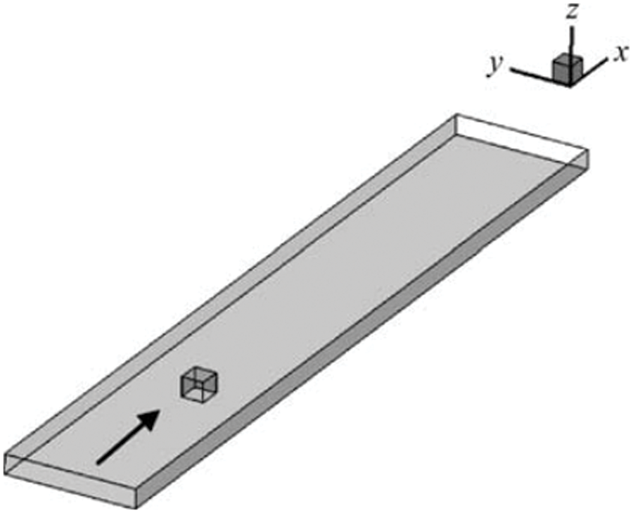
Figure 1: Three-dimensional view of single pier geometric model

3.1 Simulation of the Standard k-ε Model

1)   Criterion k−ε simulates the change of free water surface. When the flow rate is 144 m3/h, and the outlet water depth is 15 cm, the contour map of the free surface water level is shown in Fig. 2a. There was stagnant water upstream of the bridge pier, and the maximum inactive water height was 0.35 cm. It appears within the range of 10 cm × 10 cm directly upstream of the bridge pier [7]. The height of the backwater in most areas upstream of the piers is in the range of 0.1∼0.2 cm. The water level decreases on both sides and downstream of the bridge piers, and the maximum decrease is 0.3 cm. It is located near both sides of the bridge pier, with a range of 10 cm × 10 cm.

Figure 2: Standard simulated free surface water level contour

In addition, a significant drop in the water level can also be observed in the corresponding range of the downstream rear end of the bridge pier, and the drop in the water level is generally in the range of 0.1 cm. When the flow rate is 288 m3/h, and the outlet water depth is 15 cm, the contour map of the free surface water level is shown in Fig. 2b. Retention water is also common upstream of the bridge pier, and the maximum height of the backwater is about 0.9 cm. It appears in the middle and upper reaches of the bridge piers, with an area of 10 cm × 10 cm. The height of stagnant water upstream of the bridge piers is generally between 0.1 and 0.5 cm. This is a significant increase compared to the flow rate of 144 m3/h under the same model. The water level decreases downstream and on both sides of the pier, and the maximum decrease is 0.9 cm. Under this condition, the water level decrease in most areas downstream of the pier exceeding 0.3 cm.

2)   The change of the average flow rate: In the case of a flow rate of 144 m3/h and an outlet depth of 15 cm, the vertical average flow velocity contour diagram is shown in Fig. 3a. The flow velocity in a local upstream area of the bridge pier is reduced due to the backwater, and the maximum value of the reduction is 0.17 m/s. The affected area is located in the range of 10 cm × 10 cm upstream of the middle pier. The flow velocity increases on both sides of the pier due to the squeezing water flow [8]. The maximum increase in velocity is 0.038 m/s. Due to the water blocking effect of the pier, the flow velocity decreases in a larger area downstream of the pier. The maximum reduction is 0.21 m/s. When the flow rate is 288 m3/h, and the outlet water depth is 15 cm, the vertical average flow velocity contour diagram is shown in Fig. 3b. The maximum value of the flow velocity reduction in front of the pier is 0.34 m/s. The velocity reduction range upstream of the pier is between 0.04 and 0.34 m/s. The decrease in the flow velocity is greater than the case of the flow rate of 144 m3/h under the same model [9]. The flow velocity on both sides of the bridge pier increased significantly, and the maximum increase was 0.1 m/s. The flow velocity downstream of the bridge pier has a large decrease, and the maximum value of the decrease is 0.41 m/s.

Figure 3: Schematic diagram of standard k−ε simulated vertical average velocity

3.2 Simulation of RNG k-ε Model

1)   Free surface water level analysis: When the flow rate is 144 m3/h, and the outlet water depth is 15 cm, the contour map of the free surface water level is shown in Fig. 4a. Upstream of the bridge, piers all appear with backwater, and the height of the backwater is symmetrical. The maximum value of backwater is 0.2 cm. It is located at the upstream front end on both sides of the bridge pier. In addition, the obvious high-water level can also be observed in the corresponding range of the upstream front end of the middle and upstream of the bridge piers. The height of the backwater is between 0.1∼0.2 cm. The water level drops on both sides and downstream of the bridge piers. The maximum reduction value is 0.3 cm near the piers on both sides [10]. The range is 10 cm × 10 cm, respectively. In addition, a significant drop in water level can also be observed in the corresponding range of the downstream rear end of the bridge pier. The range of the water level droppage is generally between 0.1 and 0.2 cm. When the flow rate is 288 m3/h, and the outlet water depth is 15 cm, the contour map of the free surface water level is shown in Fig. 4b. The upstream backwater range is between 0.2∼0.8 cm, and the maximum backwater value appears directly upstream of the pier. It appears in the area of 10 cm × 10 cm. The height of the upstream backwater is higher than the upstream backwater height with the flow rate of 144 m3/h under the same model [11]. Large-scale water drops occurred on both sides and downstream of the bridge piers. In most downstream areas, the water level decreased in the range of 0.2 to 0.8 cm, and the maximum water level decrease was 1.1 cm and appeared downstream of the bridge pier.

Figure 4: RNG k−ε simulated free surface water level contour

2)   Analysis of average flow rate: When the flow rate is 144 m3/h, and the outlet water depth is 15 cm, the vertical average flow velocity contour diagram is shown in Fig. 5a. The flow velocity in a local upstream area of the bridge pier is reduced due to stagnant water, and the maximum value of the reduction is 0.17 m/s. This are is located within the range of 10 cm × 10 cm upstream of the pier. As the water flow area decreases on both sides of the bridge piers and between the bridge piers, the flow velocity increases [12]. The maximum increase in flow velocity is 0.065 m/s. The flow velocity decreases downstream of the pier, and the maximum value of the decrease is 0.2 m/s. The reduced area is mainly at the end of the pier. When the flow rate is 288 m3/h, and the outlet water depth is 15 cm, the vertical average flow velocity contour diagram is shown in Fig. 5b. The flow velocity upstream of the bridge pier shows the same law as the flow rate of 144 m3/h under the same model, but the maximum value of the flow velocity reduction reaches 0.34 m/s. This is greater than the flow rate of 144 m3/h under the same model. When the maximum increase in flow velocity is 0.11 m/s, it appears in the downstream area on both sides of the pier. The maximum reduction is 0.42 m/s. This are is mainly located at the end of the middle pier. The velocity reduction value in other areas is between 0.04 and 0.39 m/s.

Figure 5: Schematic diagram of RNG k−ε simulated vertical average velocity

3.3 k-ε Model Can be Simulated

1)   Free surface water level analysis: When the flow rate is 144 m3/h, and the outlet water depth is 15 cm, the contour map of the free surface water level is shown in Fig. 6a. There is backwater upstream of the bridge pier, and the maximum value of backwater is 0.2 cm. In addition, there was a drop in the water level downstream of the pier [13]. The maximum water level drop was 0.4 cm and appeared in the range of 10 cm × 10 cm on the right side of the pier. The downstream water level generally decreases in the range of 0.1∼0.3 cm. When the flow rate is 288 m3/h, and the outlet water depth is 15 cm, the contour map of the free surface water level is shown in Fig. 6b. The backwater phenomenon appeared upstream of the pier, and the maximum height of the backwater reached 0.9 cm and appeared in the area of 5 cm × 5 cm upstream of the pier. This is significantly higher than the flow rate of 144 m3/h under the same model. The water level downstream of the bridge piers generally decreases, and the decrease range is between 0.2∼0.9 cm.

Figure 6: k−ε simulated free surface water level contour can be realized

2)   Analysis of average flow rate: When the flow rate is 144 m3/h, and the outlet water depth is 15 cm, the vertical average flow velocity contour diagram is shown in Fig. 7a. The flow velocity in a local upstream area of the bridge pier is reduced due to stagnant water. The reduction range is between 0.02∼0.17 m/s. The water flow area decreases on both sides of the pier, increasing flow velocity [14]. The maximum increase in flow velocity is 0.08 m/s. The flow velocity decreases downstream of the pier, and the maximum value of the decrease is 0.21 m/s. The reduced area is within a larger range at the end of the pier. When the flow rate is 288 m3/h, and the outlet water depth is 15 cm, the vertical average flow velocity contour diagram is shown in Fig. 7b. The upstream flow velocity generally decreases, and the maximum value of the decrease is 0.31 m/s. It is located directly upstream of the pier. The area with the largest increase in velocity is located downstream on both sides of the pier, and the maximum increase is 0.15 m/s. At the same time, the flow velocity is greatly reduced downstream of the pier, and the maximum reduction is 0.42 m/s.

Figure 7: Schematic diagram of k−ε simulation of average vertical velocity

3.4 Comparison and Analysis between the Results of Mathematical Simulations of Three Turbulence Models and the Measured Results

Based on some hydraulic characteristics of the water movement near the bridge piers, we compared the calculation results mainly from the free surface water level change, the average flow velocity, the wake vortex shape, and the upstream cross-sectional water level change with the measured data [15].

Fig. 8 shows the experiment with two cross-sections taken at the distance of 4.8 m and 4.9 m from the inlet, respectively, when the flow rate is 144 m3/s. We use three turbulence models to simulate the water level of the cross-section near the single pier and the comparison chart of the measured water level. It can be seen from Fig. 8 that there is a big difference between the simulation results of the standard k−ε model and the measured results when the water surface is simulated. Both the RNG k−ε model and the achievable k−ε model can simulate the free water surface well.

Figure 8: Cross-sectional water level comparison when the flow rate is 144 m3/h

Fig. 9 is a comparison diagram of the vertical average velocity contours near a single pier simulated using three turbulence models at a flow rate of 144 m3/s and the actual measured velocity [16]. The points of different shapes in the figure represent the distribution of different flow velocity points. It can be seen from the figure that scheme 1 (standard k−ε ) has a large deviation from the measured data in the simulation of flow velocity. In contrast, scheme 2 (RNG k−ε ) and scheme 3 (achievable k−ε ) can better simulate the distribution of flow velocity.

Figure 9: Comparison of average flow velocity and measured flow velocity of 144 m3/s

3.5 Comparison of Mathematical Simulation Results of Three Turbulence Models

Under the same model, with the flow rate increase, the maximum value of the decrease of the flow velocity presents the same change law as the maximum height of the backwater. There is an unstable flow state at the end of the pier [17]. The boundary layer will be forcibly separated near the singularity. The vortex shedding occurs at the sharp corners of the square column surface and gradually develops into a more mature Karman vortex at the tail. From the comparison of the free surface water level, the average vertical velocity, and the experimental data, it can be seen that the RNG k−ε model and the achievable k−ε model are better than the standard k−ε model in the simulation of water surface and velocity near a single pier. All three models can achieve good results in the simulation of the tail flow field. Therefore, in general, the RNG k−ε model and the achievable model can better simulate the water flow near a single pier.

4  Conclusion

The flow rate of the stagnant water upstream of the bridge pier decreases. The squeezing water flow on both sides of the bridge piers and between the bridge piers causes the flow velocity to increase. Due to the water blocking effect of the bridge piers, the flow velocity at the end of the bridge piers decreases more. In the same model, with the flow rate increase, the maximum value of the flow rate decrease shows the same change law as the maximum height of the backwater.

Acknowledgement: The author would like to extend his(her) thanks to the learning and research platform, as well as the generous financial support provided by the company and the school.

Funding Statement: The author received no specific funding for this study.

Conflicts of Interest: The research topic of this article is independently completed by the author’s team, and does not involve any conflict of interest issues.

References

1. He, S., Yan, S., Deng, Y., Liu, W. (2019). Impact protection of bridge piers against rockfall. Bulletin of Engineering Geology and the Environment, 78(4), 2671–2680. DOI 10.1007/s10064-018-1250-5. [Google Scholar] [CrossRef]
2. Wang, C. (2021). Overview of integrated health monitoring system installed on cable-stayed bridge and preliminary analysis of results. Građevinar, 73(6), 591–604. [Google Scholar]
3. Liu, X., Gui, N., Wu, H., Yang, X., Tu, J. (2020). Numerical simulation of flow past stationary and oscillating deformable circles with fluid-structure interaction. Experimental and Computational Multiphase Flow, 2(3), 151–161. DOI 10.1007/s42757-019-0054-6. [Google Scholar] [CrossRef]
4. Elsaady, W., Ibrahim, A., Abdalla, A. (2019). Numerical simulation of flow field in coaxial tank gun recoil damper. Advances in Military Technology, 14(1), 139–150. DOI 10.3849/AiMT. [Google Scholar] [CrossRef]
5. Deng, Z., Wang, C., Yao, Y., Higuera, P. (2020). Numerical simulation of an oscillating water column device installed over a submerged breakwater. Journal of Marine Science and Technology, 25(1), 258–271. DOI 10.1007/s00773-019-00645-0. [Google Scholar] [CrossRef]
6. Karadimou, D. P., Papadopoulos, P. A., Markatos, N. C. (2019). Mathematical modelling and numerical simulation of two-phase gas-liquid flows in stirred-tank reactors. Journal of King Saud University-Science, 31(1), 33–41. DOI 10.1016/j.jksus.2017.05.015. [Google Scholar] [CrossRef]
7. Jin, X., Laima, S., Chen, W. L., Li, H. (2020). Time-resolved reconstruction of flow field around a circular cylinder by recurrent neural networks based on non-time-resolved particle image velocimetry measurements. Experiments in Fluids, 61(4), 1–23. DOI 10.1007/s00348-020-2928-6. [Google Scholar] [CrossRef]
8. Al-Obaidi, A. R. (2020). Investigation of the influence of various numbers of impeller blades on internal flow field analysis and the pressure pulsation of an axial pump based on transient flow behavior. Heat Transfer, 49(4), 2000–2024. DOI 10.1002/htj.21704. [Google Scholar] [CrossRef]
9. Yu, D., Tang, L., Chen, C. (2020). Three-dimensional numerical simulation of mud flow from a tailing dam failure across complex terrain. Natural Hazards and Earth System Sciences, 20(3), 727–741. DOI 10.5194/nhess-20-727-2020. [Google Scholar] [CrossRef]
10. Düzel, Ü., Schroeder, O. M., Zhang, H., Martin, A. (2020). Numerical simulation of an Arc Jet test section. Journal of Thermophysics and Heat Transfer, 34(2), 393–403. DOI 10.2514/1.T5722. [Google Scholar] [CrossRef]
11. Le, T. B., Khosronejad, A., Sotiropoulos, F., Bartelt, N., Woldeamlak, S. (2019). Large-eddy simulation of the Mississippi River under base-flow condition: Hydrodynamics of a natural diffluence-confluence region. Journal of Hydraulic Research, 57(6), 836–851. DOI 10.1080/00221686.2018.1534282. [Google Scholar] [CrossRef]
12. Harada, E., Ikari, H., Khayyer, A., Gotoh, H. (2019). Numerical simulation for swash morphodynamics by DEM–MPS coupling model. Coastal Engineering Journal, 61(1), 2–14. DOI 10.1080/21664250.2018.1554203. [Google Scholar] [CrossRef]
13. Sun, X. W., Liu, W., Chai, Z. X. (2019). Method of investigation for numerical simulation on aero-optical effect based on WCNS-E-5. AIAA Journal, 57(5), 2017–2029. DOI 10.2514/1.J057961. [Google Scholar] [CrossRef]
14. Ma, Y., Rashidi, M. M., Yang, Z. G. (2019). Numerical simulation of flow past a square cylinder with a circular bar upstream and a splitter plate downstream. Journal of Hydrodynamics, 31(5), 949–964. DOI 10.1007/s42241-018-0087-5. [Google Scholar] [CrossRef]
15. Ghalandari, M., Mirzadeh Koohshahi, E., Mohamadian, F., Shamshirband, S., Chau, K. W. (2019). Numerical simulation of nanofluid flow inside a root canal. Engineering Applications of Computational Fluid Mechanics, 13(1), 254–264. DOI 10.1080/19942060.2019.1578696. [Google Scholar] [CrossRef]
16. Liu, E., Guo, B., Lv, L., Qiao, W., Azimi, M. (2020). Numerical simulation and simplified calculation method for heat exchange performance of dry air cooler in natural gas pipeline compressor station. Energy Science & Engineering, 8(6), 2256–2270. DOI 10.1002/ese3.661. [Google Scholar] [CrossRef]
17. Issakhov, A., Zhandaulet, Y. (2019). Numerical simulation of thermal pollution zones’ formations in the water environment from the activities of the power plant. Engineering Applications of Computational Fluid Mechanics, 13(1), 279–299. DOI 10.1080/19942060.2019.1584126. [Google Scholar] [CrossRef]
Cite This Article
Copyright © 2023 The Author(s). Published by Tech Science Press.
This work is licensed under a Creative Commons Attribution 4.0 International License , which permits unrestricted use, distribution, and reproduction in any medium, provided the original work is properly cited.
Downloads
Citation Tools