Dynamic Analysis of Pipeline Lifting Operations for Different Current Velocities and Wave Heights

1  Introduction

With the further development of the offshore oil industry, offshore oil and gas transportation are becoming more and more prosperous as well [1,2]. The pipeline transportation system plays an increasingly prominent role in oil and gas transportation and has been widely used in developing offshore oil fields [3,4]. It is also the most practical type of deep-sea offshore oil system [5]. The pipeline system typically consists of a surface vessel, lifting pipe, lifting pump sets, buffer, lifting hose, and subsea collector [6,7]. In this system, the lifting pipe must be equipped with pump sets for lifting the mineral resources to the vessel and a buffer to regulate the density of the oil-water mixture.

The pipeline stress-strength analysis is an important stage in overall construction design [8]. In mechanical analysis, the deformation and stress analysis of pipelines in the process of laying, sinking, and lifting are the key problems. During the lifting or sinking stage, one end of the pipeline is placed on the seabed, the other is lifted and suspended, and the middle suspension span is long, as shown in Fig. 1. The stress of the pipeline is complex, and the bending deformation is great. Therefore, in order to ensure that the deformation of the pipeline during laying or lifting is controlled within the elastic deformation range, it is necessary to conduct stress analysis on the pipeline sections at different heights to determine the deformation of the pipeline itself or to change the construction parameters to ensure that the deformation of the pipeline is controlled within the elastic deformation range. Therefore, the analysis of the mechanical properties of the suspended pipeline is the key to the construction analysis of the pipeline.

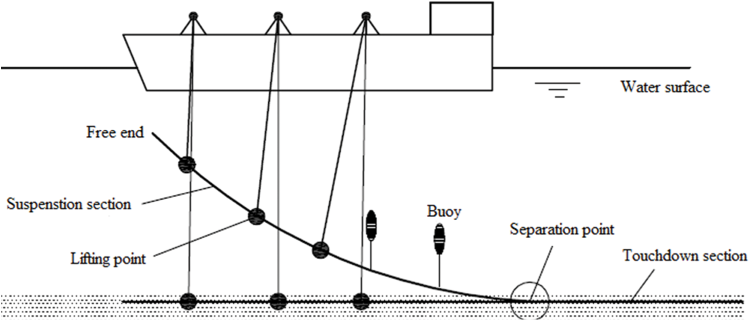
Figure 1: Pipeline lifting construction field [9]

Scholars have done a lot of research on the mechanical behavior of the pipeline already. For example, Preston et al. [10] reported and analyzed a new pipeline global buckling control method by laying a pipeline with a zig-zag shape to trigger controllable mitigatory lateral global buckling. Polak et al. [11] studied the influence of the curvature radius of the curved segment and pipeline stiffness on pipeline load. Cheng et al. [12] elaborated a theoretical model of the pull-back pipeline. Wu et al. [13] tested the pipeline’s mechanical behavior in the pipeline laying process through experimental methods, and the experiment test results are compared with the theoretical results. Guo et al. [9] used the continuous beam theory to analyze the mechanical behavior of pipelines during lifting construction and implemented the mechanical model of pipelines during the lifting construction process. The analysis showed that the lifting height varies linearly with the pipeline length. Liu et al. [14–16] carried out a series of research on pipe lifting projects in horizontal directional drilling. Their research has guiding significance for the actual engineering implementation of the pipeline lifting operation. Hong et al. [17] analyzed the feature of lifting deformation for a pipeline laid on a sleeper and studied nine influential factors of the variation in the lifting displacement. Zan et al. [18] proposed a coupled time-domain numerical model for the behavior study of pipeline laying. The model was solved by the Newmark method and verified with OrcaFlex software. Chung [19] conducted offshore tests of deep-sea mining systems to measure the response of full-scale pipelines. Guo et al. [20] studied the effect of pipeline surface roughness on the interaction between submarine landslides and pipelines. The effect of surface roughness is primarily reflected in the peak load of the impact forces on the pipelines. Puckett [21] used a new theoretical method to calculate the pull-back load in process of pull-back pipeline. Podbevsek et al. [22] proved that the pipeline has a large reaction force in the curved segment through a theoretical method. Erol [23] established the dynamic model of the stepped lifting pipe, and studied the longitudinal vibration characteristics of the lifting system with and without dynamic vibration absorber by using the method of separating variables. Prpíc-Ořsíc et al. [24] made a related study of the interaction between the submarine pipeline and construction vessel by nonlinear differential equations with the Runge-Kutta method, in which the extension of the general two dimensional formulations of pipeline dynamics was presented by accounting for the effects of wave excitation, cable/ship interaction and cable elasticity. Reda et al. [25] showed the process for the simulation of the pipeline laying tension and bending radius in OrcaFlex. Then the simulation models in OrcaFlex and compression test for compression limit state of HVAC submarine pipeline were made by Reda et al. [26].

As can be seen from the brief review of the most advanced research, the current research on the mechanical behavior of the pipeline focuses on modeling and simulation analysis of the whole deep-sea system cooperative operation, the dynamic characteristics analysis of the lifting pipe, and the process of laying from water surface to seabed [27–31]. However, there are few reports on the dynamic analysis of the pipeline lifting operation. In pipeline construction and maintenance, lifting the submerged pipeline to the sea surface is often necessary, weld and inspect the pipeline or riser joint for further laying or maintenance. At this stage, due to the large deflection deformation, the complex environment and working load such as wind and waves, the pipeline will produce great bending stress, which makes the pipeline vulnerable to serious damage. Therefore, the mechanical analysis at this stage is very important for the laying and construction of the pipeline.

In this paper, the pipeline lifting operation is modeled in OrcaFlex, and the hydrodynamic response in the process of pipe lifting is calculated by the time-domain coupling dynamic analysis method. To ensure the authenticity of the simulation to the greatest extent, the simulation time step must be less than the period of the shortest natural node. It should not exceed 1/10 of the shortest natural period of the model. Combined with the calculation results of hydrodynamic performance then, some guiding suggestions are given.

2  The Theoretical Model

When the lifting force is applied to a pipeline, the pipeline will deflect. In an actual engineering project, compared with the length of the pipe section to be lifted, the lifting height and angle change is minimal. Therefore, the small deflection linear theory can be used to calculate the deflection of the pipeline. The lifting process is a problem of moving boundaries in the pullback step, so a multipoint lifting model of the pipeline can be built using a polynomial interpolation function. To find the position of the moving boundary, the displacement correction methods, such as load concentration correction, horizontal spacing correction, and iterative calculation, are used to convert the large deformation geometric nonlinear problem of the pipeline to a piecewise linear problem [32].

2.1 Mechanical Model

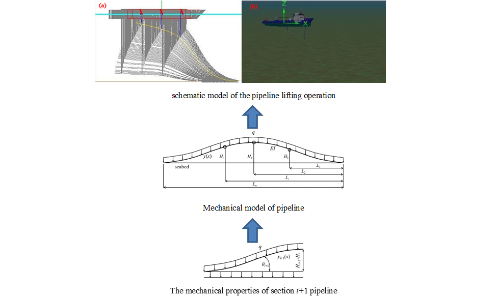
Fig. 2 shows the mechanical model. The uniform weight q is applied to the pipeline. Hi and Li represent each point’s vertical and horizontal displacements, respectively. If the pipeline is segmented according to the pipeline’s endpoints and lifting points, the bending deformation is small.

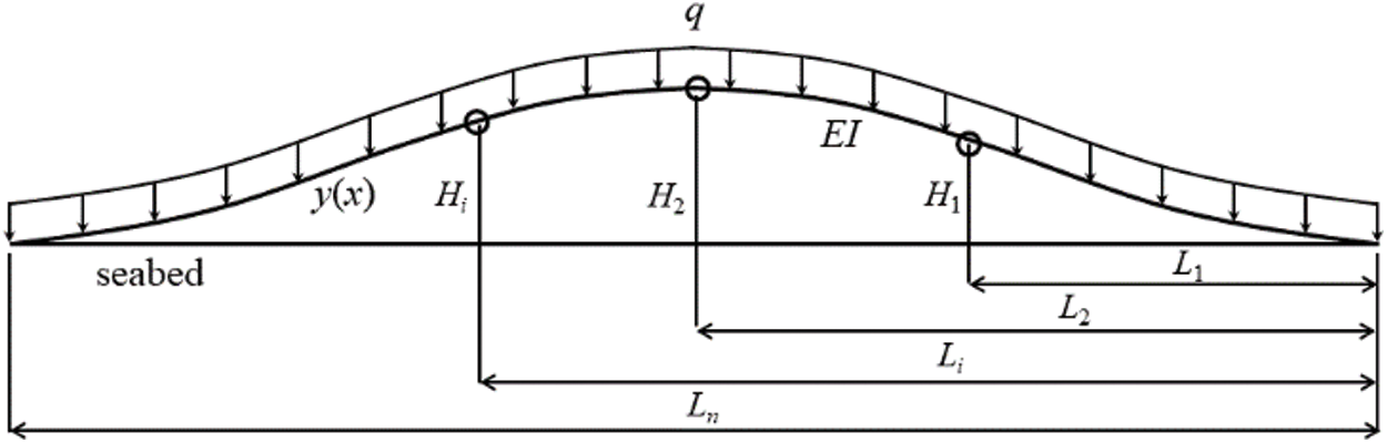
Figure 2: Mechanical model of pipeline

Based on the small deflection beam theory, the relationship among the physical parameters is as follows:

Corner:

θ=dydx (1)

Bending moment:

M=EId2ydx2 (2)

Uniform load:

q=EId4ydx4 (3)

Selecting the linear interpolation function as the calculation equation, the differential equation for bending deformation is as follows:

d4y1dx4=qEI (4)

The solution of the Eq. (4) is as follows:

y1(x)=a10+a11x+a12x2+a13x3−q1x424EI (5)

The interpolation function of section i + 1 is as follows:

yi+1(x)=yi(x)+ai+10+ai+11(x−Li)+ai+12(x−Li)2+ai+13(x−Li)3−qi+1(x−Li)424EI (6)

where, ai+10, ai+11, ai+12, ai+13 represent the unknown coefficients, Li represents the horizontal coordinate value of point x, yi+1(x) and yi(x) represent the boundary point of interpolation functions, qi+1 represents the weight increment of segment i + 1. At the same time, Fig. 3 shows the mechanical properties of the section, calculated as follows:

qi+1=qcosθ(i+1)−qcosθ(i),i=1,2,…,n (7)

where, θ(i + 1) represents the angle formed by the horizontal and oblique line calculated by points i and i + 1, as does θ(i).

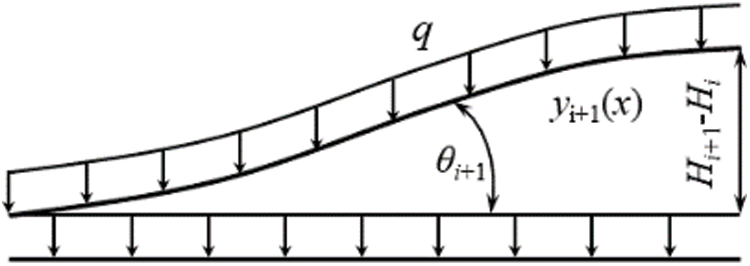
Figure 3: The mechanical properties of section i + 1 pipeline

According to the mechanics of materials, the deflection angle is 0, corner is 0, and bending moment is 0 at the ending point of the pipeline. Then the following equation can be gotten, y(0) = y′(0) = y′′(0) = 0. So the following equations can be written at the boundary points:

yi+1(Li)=yi(Li),yi+1′(Li)=yi′(Li),yi+1′′(Li)=yi′′(Li) (8)

The ai0, ai1, ai2 (i = 1, 2, …, n) can be gotten by solving these equations. Therefore, Eqs. (5) and (6) can be transformed as follows:

y1(x)=a3x3−q1x424EI (9)

yi(x)=yi−1(x)+ci(x−Li−1)3−qi(x−Li−1)424EI,i=1,2,…,n (10)

After the simplification, there are still some unknown coefficients which can be calculated according to the lifting height of each point and the pipeline ending point Hi. Since the pipeline is gimbaled at the end point of the pipeline which means the bending moment is 0, the additional condition is as follows:

Mn=EId2yndx2 (11)

The value of parameter Ai is as follows:

Ai=Hi−yi−1(Li)+qi(Li−Li−1)4/24EI(Li−Li−1)3 (12)

The interpolation function of each segment is as follows:

yi(x)=yi−1(x)+Hi−yi−1(LI)+qi(Li−Li−1)424EI(Li−Li−1)3(x−Li−1)3−qi(x−Li−1)424EI,i=2,3,…,n (13)

The angle and moment can be gotten by solving Eq. (13), and the distance L1 can be known according to the following equation:

yn′′(Ln)=yn−1′′(Ln)+6Hn−yn−1(Ln)+qn(Ln−Ln−1)4/24EI(Ln−Ln−1)2−qn(Ln−Ln−1)22EI=0 (14)

After calculating the deflection curve of the pipeline, the equations of the rotation angle, bending moment and shear force of each pipeline segment can be obtained according to the linear beam theory:

θi(x)=yi′(x) (15)

Mi(x)=EIyi′′(x) (16)

Qi(x)=Mi′(x)=EIyi′′′(x) (17)

After obtaining the interpolation function, the maximum stress can be calculated using the following equation:

σmax=MmaxW (18)

where, W represents the section bending modulus, W = I/ymax; I represents the moment of inertia, I = π(D4 − d4)/64; ymax represents the maximum deflection.

Using the deflection equation of the last segment yn and boundary conditions at the ending point then, the corresponding angle can be obtained:

θ=yn′(x)|x=Ln=yn′(Ln)=yn−1′(Ln)+3Hn−yn−1(Ln)+qn(Ln−Ln−1)4/24EI(Ln−Ln−1)−qn(Ln−Ln−1)36EI (19)

2.2 Marine Environmental Load

Due to the particularity of the marine environment, the load on the subsea pipeline system is relatively complex. For subsea pipelines, waves and currents are the most important external loads. Since the pipe lifting operation is rarely carried out under strong wind conditions, to save calculation time, the wind load is not considered in this paper.

When calculating and analyzing the pipeline, it is assumed that the pipeline is a flexible structure. The calculation and analysis mainly include the axial tension borne by the pipeline, the action of environmental load, and the coupling dynamic response of the whole system. The lump-mass method is used for modeling. The performance of the pipeline is equivalent to a nonlinear spring, which is discretized into the lump-mass model [33]. The pipeline is simulated as a combination of axial, rotating spring, and damper. The node concentrates half of the mass of two adjacent segments, and the force and moment act on the node, which is the mathematical basis for establishing the pipeline load calculation model in OrcaFlex.

The wave and current forces on the submarine pipeline can be calculated by the Morrison equation:

Normal component of current force:

Fnc=12CnρDνn2 (20)

Tangential component of current force:

Ftc=12CtρDνn2 (21)

Normal component of wave force:

Fnw=12CnρDun2+CmρπD24∂u∂t (22)

Tangential component of wave force:

Ftw=12CtρDut2 (23)

where, Cn is the normal drag coefficient, Ct is the tangential drag coefficient, the numerical value of the drag coefficient changes with Reynolds number; Cm is the inertia force coefficient, the numerical value is 2; vn = v⋅sinθ, vt = v⋅cosθ, they are the normal velocity and tangential velocity of the current, respectively; un = u⋅sinθ, ut = u⋅cosθ, they are the normal velocity and tangential velocity of the current, respectively.

As an important marine environment load, the submarine surface sediments will also affect the dynamic behavior of the pipeline lifting operation [34]. The undrained shear strength is the main characteristic of the submarine surface sediments. In pipeline lifting operation, the undrained shear strength of surficial marine clays is a significant parameter for engineering construction and geological disaster assessment [35]. In this paper, the submarine surface is considered non-smooth.

The hydrodynamic analysis includes static and dynamic analysis. Static analysis has two main functions: to analyze whether the system structure reaches static equilibrium under the action of gravity, buoyancy, and flow viscosity. The other is to provide an initial state for dynamic analysis.

The dynamic analysis starts from the steady-state provided by static analysis. It includes the self-construction stage and model maintenance analysis stage. The self-construction stage is where the wave and ship motion gradually increase from static to the given value. This stage generally requires a wavelength of time. After the self-construction stage, the model can enter the maintenance analysis stage. The dynamic simulation calculation adopts two sets of explicit and implicit calculation methods. Both calculate the system’s geometric shape at each time step and fully consider the nonlinear geometric factors, including the spatial variation of wave load and contact load. The equation of motion is solved by explicit forward Euler integration with a fixed step size. The initial model parameters are obtained through static analysis to calculate the forces and moments of each free body and node, including gravity, buoyancy, hydrodynamic and air resistance, hydrodynamic added mass, tension and shear force, bending moment, seabed friction, object contact force, the force exerted by hinge and winch, etc.

2.3 The Discrete Numerical Method

The numerical solution of the boundary problem for the pipeline is the discrete lumped mass method [36]. The basic idea of this model is to divide the pipeline into N segments, and the mass of each element is concentrated on one node, so that there are N + 1 nodes. The tension T and shear V acting at the ends of each segment can be concentrated on a node, and any external hydrodynamic load is concentrated on the node. The equation of motion of i-th node (i = 0, 1,…,N) is:

MAiR¨i=Tei−Tei−1+FdIi+Vi−Vi−1+wiΔs¯i (24)

Among them, R represents the node position of the pipeline.

MAi=Δs¯i(mi+π4Di2(Can−1))I−Δs¯iπ4Di2(Can−1)(τi⊗τi−1) is the mass matrix of a node, I is a 3 × 3 identity matrix; Tei=EAεi=EAΔs0iΔsεi , which stands for effective tension at a certain node; Δs0i=L0(N−1) , which represents the original length of each segment; Δsεi=|Ri+1−Ri| , the stretched length of each segment; EA, axial stiffness of the pipeline.

FdIi represents the external hydrodynamics of each node, which is calculated according to the Morison equation:

FdIi=12ρDi1+εiΔs¯i(Cdni|vni|vni+πCdti|vti|vti)+π4Di2ρCaniΔs¯i(awi−(awi⋅τi))τi (25)

where, ρ is the density of sea water, Di is the diameter of each cable, Cdni is the normal drag coefficient, Cdti is the tangential drag coefficient, Cani is the inertia coefficient. Vi=EIi+1τi×(τi×τi+1)ΔsεiΔsεi+1−EIiτi×(τi−1×τi)Δsεi2+Hi+1τi×τi+1Δsεi , V represents the shear force at the node, H is the torsion.

The lumped mass model is shown in Fig. 4.

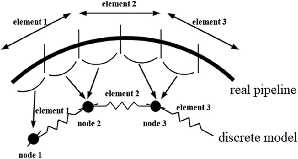
Figure 4: The lumped mass model

In OrcaFlex, there are two temporal discretization schemes, explicit and implicit integrations. The explicit time integration takes a constant time step to integrate forward. At the beginning of the simulation, after a preliminary static analysis, the initial positions and orientations of all nodes in the model are known. The forces and moments of all free bodies and nodes are calculated, including gravity, buoyancy, hydrodynamic force, hydrodynamic added mass, tension and shear, bending and moment, seabed friction, etc.

The motion control equation for each free body and node in the model is as follows:

M(s)a=F(s,v,t)−C(s,v)−K(s) (26)

where, s, v, a, t represent the displacement, velocity, acceleration and time, respectively. M, F, C, K represent the mass, load, drag force, and stiffness, respectively.

For implicit integration, the generalized-α method is used in OrcaFlex [37]. Forces, moments, damping, weight are calculated in the same way as explicit integration. Since the forces, displacements, velocities, and accelerations are unknown at the last time step, an iterative approach is required. To improve computational efficiency, a pre-simulation stage is usually preset in OrcaFlex. The simulation time at this stage is set to be no less than one wave period. In the modeling preparation stage, the wave dynamic parameters, ship motion and current parameters are increased from 0 to a fixed value. In this way, the simulation can have a smooth start, reduce transient response and avoid long simulation runs.

Although it is easy to achieve stability using implicit integration, the corresponding calculation results are often inaccurate. For rapidly changing physical phenomena, such as fast collisions, more attention should be paid to the accuracy of the calculation results. In this case, it is necessary to compare the calculation results of the implicit and explicit integration formats in order to study the sensitivity of the time step. Both methods recalculate the geometry of the system after each time step, so the numerical simulations are adequate for geometric nonlinearities, including spatial variations of wave loads and contact loads. The time domain simulation steps in this paper are shown in Fig. 5.

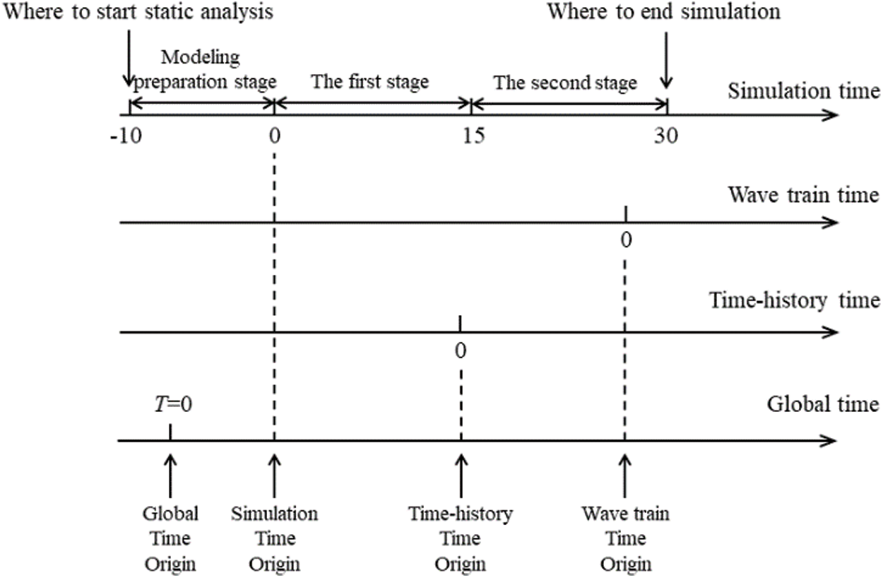
Figure 5: The time domain simulation steps

3  Numerical Model Set-Up

3.1 Coordinate System

The coordinate system can be divided into the global coordinate system and vessel coordinate system. Both use the right-hand coordinate system. The origin of the global coordinate system is set on the sea level, the Z direction is vertical upward, and the X and Y directions meet the right-hand rule. The coordinate vessel system is generally used when establishing the numerical model. When determining the position of the global model, the global coordinates are adopted. In this paper, the position of the whole model is determined regarding the global coordinates. The global and coordinate vessel system is shown in Fig. 6. The direction and headings of waves and currents is shown in Fig. 7.

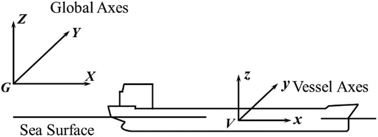
Figure 6: The global and vessel coordinate system

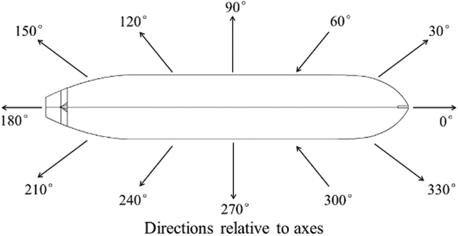
Figure 7: The direction and headings of waves and current

3.2 Model Set-Up in OrcaFlex

The upper boundary condition of the pipeline model mainly depends on the motion of the vessel to which it is connected. The motion of the vessel depends on RAOs. RAOs, known as response amplitude operators are a concept of engineering statistics in the field of ship or floating body designs, which can be used to calculate the behavior of ships working in sea conditions. Vessel RAOs can generally be obtained by model experiment or CFD (Computational Fluid Dynamics). It is usually necessary to calculate the motion of a floating body under various wave conditions. Its essence is a transfer function from wave excitation to vessel motion. In OrcaFlex, once the RAOs are determined, the vessel’s motion will be determined. The vessel length is 103 m, the width is 16 m, and the depth is 13.32 m. The design draft is 6.66 m, the transverse stability radius is 1.84 m, the longitudinal stability radius is 114 m, the displacement is 8800 T, the front projection on the water surface is 191 m2, and the side projection on the water surface is 927 m2. The square coefficient CB is 0.804, and the oment of inertia of head swing rotation is 5.83 × 109 kg.m2. The data of RAOs, wave drift force, added mass coefficient, and damping coefficient of the ship is from diffraction analysis of a 103 m long ship in a 400 m water depth pool.

The seabed has an important impact on the touchdown part of the pipeline. The seabed is non smooth. There is friction between the seabed and the pipeline touchdown area. The friction has a certain positive effect on the pipeline, which will hinder the low-frequency movement of the pipeline, that is, slow movement. However, how to accurately simulate the seabed friction is very difficult. We need the actual detection data of the seabed, which is generally unavailable. It is the seabed friction optimization model provided by OrcaFlex. The advantage of this model is straightforward. When the combined velocity V of the components in the X and Y directions of the landing cable section velocity is less than a critical value, the size of the seabed friction changes linearly. When the combined velocity V is equal to the critical value, the seabed friction reaches the maximum and then does not increase with the increase of the combined velocity.

In OrcaFlex, the parameters related to the pipeline are as follows [38]: the pipeline length is 300 m; the outer diameter is 0.4 m; the inner diameter is 0.36 m; the density is 7.85 t/m3; the unit length-weight is 0.187 t/m; the bending stiffness is 9.16 × 104 kN.m2; the axial stiffness 5.06 × 106 kN; the water depth is 100 m. The effects of current velocity and different wave heights are simulated, respectively. The range of current velocity is 0–4 m/s, and one current velocity is taken every 0.5 m/s. The wave height range is 0–3 m, and one wave height is taken every 0.5 m. The current direction and wave direction are taken as 0°.

The schematic model of the pipeline lifting operation is shown in Fig. 8.

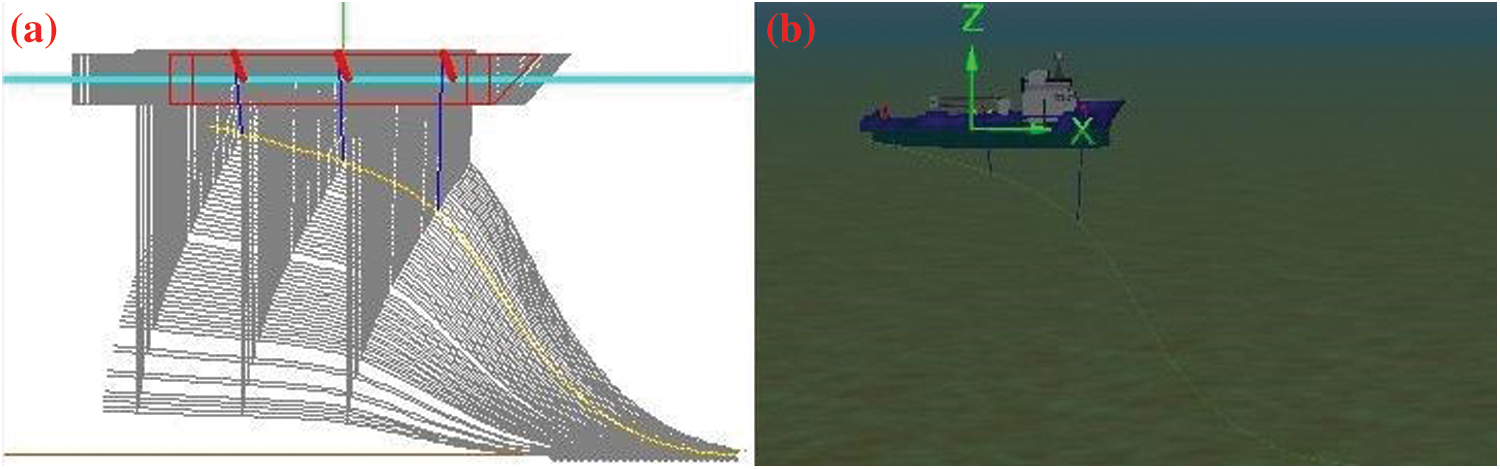
Figure 8: The schematic model of the pipeline lifting operation: (a) Simplified model in Orcaflex; (b) General schematic diagram

3.3 Validation for the Lumped Mass Method

In order to verify the correctness of the lumped mass method, a towed cable based on the mathematical formulation above is taken and let it move under the specified boundary condition [39]. The calculation results are compared with the previous results. The towed cable includes three sections: Cable, Array, Drogue. The properties of the towed cable are as shown in Table 1.

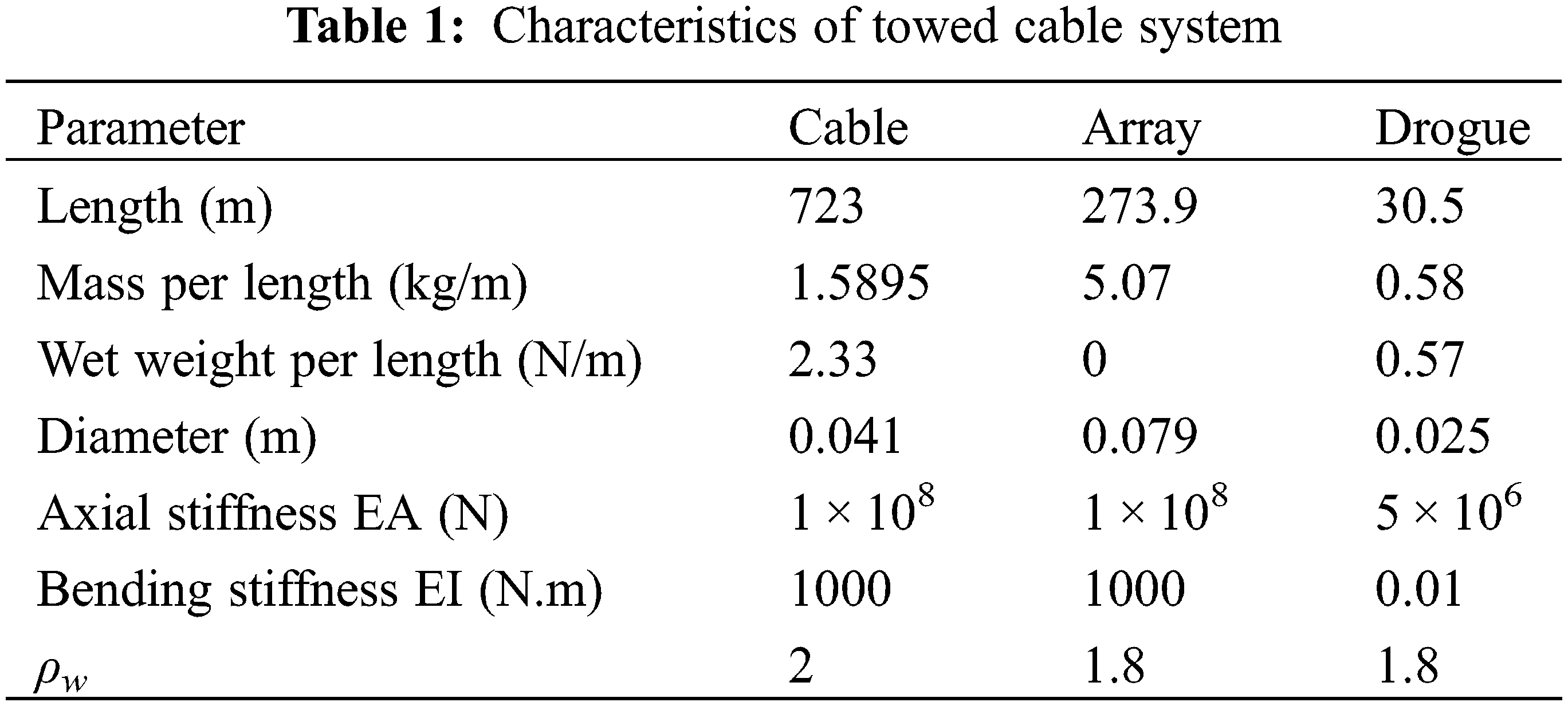
Point A which is located at 8.2 m of Array section is selected to make some comparisons between the lumped mass model and the previous research. The variations of depth of point A are compared to the results of Gobat et al. [40,41] and Ablow et al. [42]. Fig. 9 indicates that the results from the lumped mass model are consistent with the previous work, and the minimum depth of point A is closer to the measured depth. All the comparisons have validated the lumped mass method.

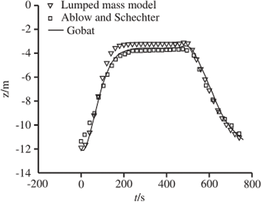
Figure 9: Validation for the lumped mass model

4  Results and Discussion

4.1 Different Wave Heights

Fig. 10 shows the changes of bending moment, curvature, and effective tension along the pipeline length at different wave heights. It is found that with the increase of wave height from 0 to 3 m, the bending moment along the length of the pipeline increases at different wave heights, but the change range is not obvious. The bending moment and curvature overlap to a large extent. As the wave height increases from 0 to 3 m, it is found in Fig. 10c that the effective tension along the length of the pipeline increases obviously with the increase of wave height.

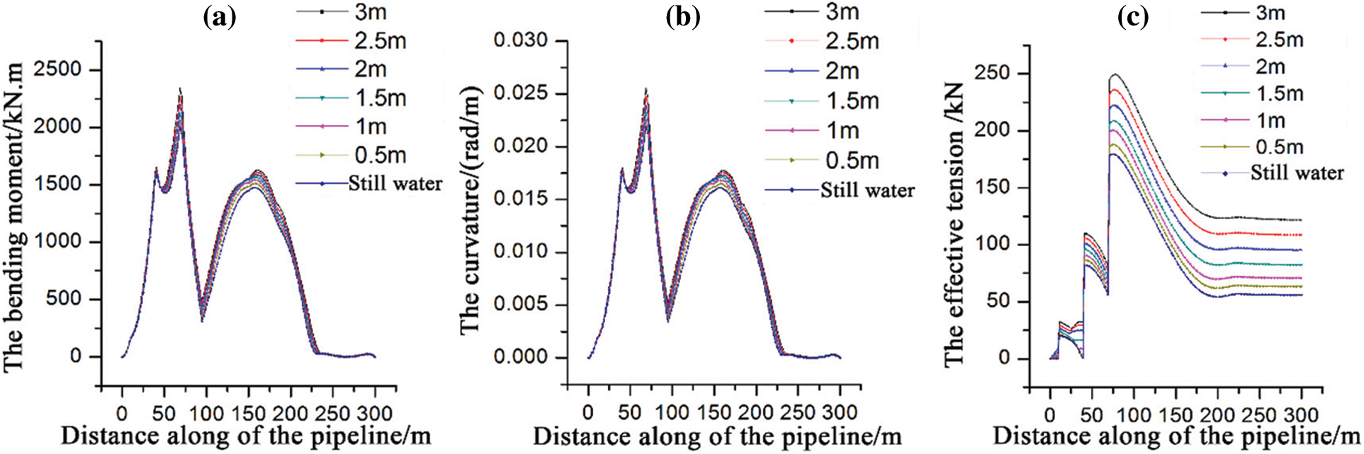
Figure 10: The results of different wave heights: (a) The bending moment; (b) The curvature; (c) Effective tension

Through observation, the bending moment, curvature, and effective tension all have sudden changes at the positions where the pipeline length is 20, 40, and 70 m. The trend is to increase sharply at first, then decrease, and then increase sharply at these three coordinate positions. Three lifting cables cause this phenomenon to facilitate operation and prevent damage to the pipeline due to the large arc bow of the pipeline during pipeline lifting. The contact position between the lifting cable and the pipeline is analyzed. The left and right of the contact point are affected by gravity and hydraulic damping. The tension along the pipeline direction increases gradually on the left of the 20 m contact point, and the tension increases sharply at the contact point due to the stress on both sides. In the section from 20 m contact point to 40 m contact point and from 40 m contact point to 70 m contact point, there is a small concave arc bow due to gravity. This arc bow is affected by the gravity component of the pipelines on both sides along the axial centerline, resulting in a compression effect, offsetting part of the tension and reducing the tension value. At the 70 m contact point, while being acted by the lifting cable and the left end pipeline, it is also acted by the gravity of the longer pipeline at the right end. Therefore, the tension and bending moment at this position are very large, which is easy to cause pipeline damage or fracture, especially when the pipeline is lifted to the highest position. At the 100 m position, the pipeline is in the transition position between the upper convex arc bow of the lifted pipeline and the lower concave arc bow of the not lifted pipeline. At this time, the pipeline becomes basically a straight segment at the critical point, and the bending moment decreases sharply. However, the tension at this position is still large due to the lifting force and the gravity of the not lifted pipeline.

4.2 Different Current Velocities

Fig. 11 shows the changes in the bending moment, curvature, and the effective tension along the length of the pipeline at different flow rates. The changes of tension and bending moment under different flow velocities are similar to the previous analysis, but there are also some special phenomena worthy of attention. In the bending moment diagram, before about 75 m along the pipeline length, the bending moment of the pipeline without flow and wave is much greater than that of the pipeline with the flow. Before the 20 m contact point, the increase of flow velocity has little effect on the effective tension of the pipeline, and the effective tension coincides within this length range. In the range of 20–70 m, the greater the velocity is, the smaller the effective tension is, showing a negative correlation phenomenon. After the 70 m contact point, there is a positive correlation between velocity and tension.

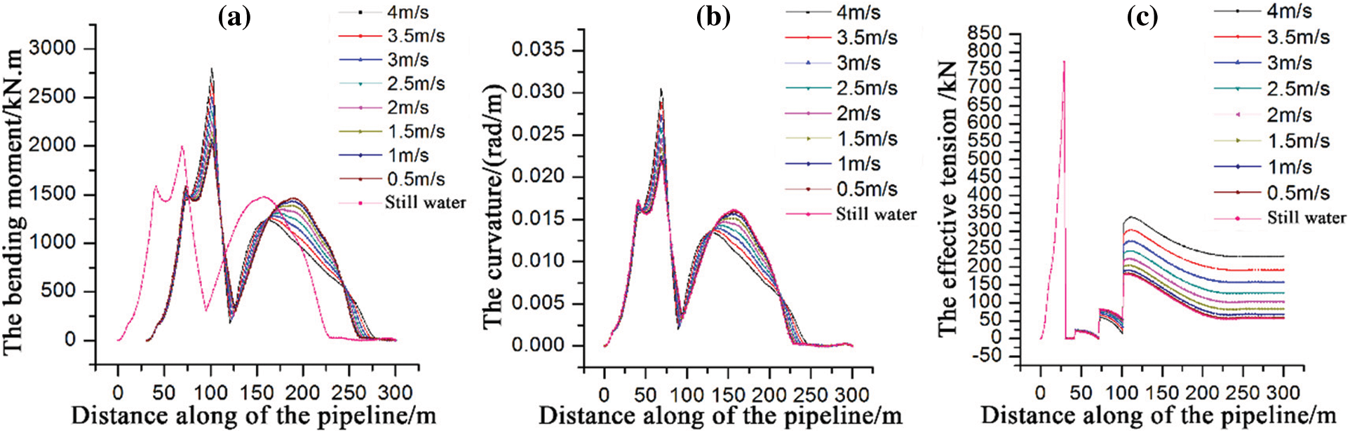
Figure 11: The results of different current velocities: (a) The bending moment; (b) The curvature; (c) Effective tension

It is not difficult to explain this phenomenon by analyzing the action process of ocean currents on pipelines. The pipeline is divided into two parts, with the 70 m contact point as the boundary. There is an upward convex arc bow in part before the 70 m contact point. After facing the current, the current generates lifting force on this section of the pipeline, balancing the tension formed by a part of the lifting cable opposite gravity’s direction the greater the flow velocity, the greater the lift that can be provided, and the better the balance effect. Therefore, the tension in this section is negatively correlated with the flow velocity. Similarly, the arc bow of this section after the 70 m contact point is concave, so the current will have a downward component on the pipeline after facing the current, which increases the tensile effect of pipe lifting operation on this section. Therefore, the greater the flow velocity, the greater the tension. This is also verified on the bending moment diagram and curvature diagram. The bending moment before and after the convex and concave transition points also has a similar trend. Still, it is opposite to the trend of tension. Before the transition point, due to the action of lift, the degree of convexity on the arc bow is deepened, and the greater the flow velocity, the greater the bending moment. After the transition point, the flow direction of the current faces the concave arc bow, which makes the alignment of this section of the pipeline close to the seabed more straight, so the bending moment decreases with the increase of velocity.

5  Conclusion

In this paper, based on the basic parameters of a certain pipeline and the specific work environment parameters, combined with the specific operation, the model of the pipeline lifting operation has been implemented by OrcaFlex. The hydrodynamic analysis under different current velocities and wave heights has been researched. This study demonstrates the following:

(1)   The changes of tension and bending moment in the process of pipe lifting obviously show the difference in the front and rear sections from the position of the bow lifting cable (the position of the 70 m contact point in the example) to the bending transition point. Therefore, before construction, it is necessary to reasonably set the lifting point in combination with the pipeline’s length and the lifting device’s position on the construction vessel.

(2)   The effect on the pipeline before and after the contact point is always one favorable and one harmful. Therefore, during construction, it is necessary to pay attention not to let the tension or bending moment of a certain section break through the safety limit.

(3)   The effects of wave heights and current velocities on the dynamic characteristics of pipeline lifting operation is mainly reflected in the effective tension. The greater the wave height and current velocity, the greater the effective tension. Although the wave in these cases has limited impact on the pipeline, considering the complexity and difficulty of the pipe lifting operation procedure, the operation in case of strong wind and waves should be avoided as far as possible.

Funding Statement: This study was financially supported by the Program for Scientific Research Start-Up Funds of Guangdong Ocean University (060302072101), Comparative Study, and Optimization of Horizontal Lifting of Subsea Pipeline (2021E05011).

Conflicts of Interest: The authors declare that they have no conflicts of interest to report regarding the present study.

References

 1.  Rui, Z., Li, C., Peng, F., Ling, K., Chen, G. et al. (2017). Development of industry performance metrics for offshore oil and gas project. Journal of Natural Gas Science and Engineering, 39, 44–53. DOI 10.1016/j.jngse.2017.01.022. [Google Scholar] [CrossRef]

 2.  Sommer, B., Fowler, A. M., Macreadie, P. I., Palandro, D. A., Aziz, A. C. et al. (2019). Decommissioning of offshore oil and gas structures-environmental opportunities and challenges. Science of the Total Environment, 658, 973–981. DOI 10.1016/j.scitotenv.2018.12.193. [Google Scholar] [CrossRef]

 3.  Zhang, S. W., Shang, L. Y., Zhou, L., Lv, Z. B. (2022). Hydrate deposition model and flow assurance technology in gas-dominant pipeline transportation systems: A review. Energy & Fuels, 36(4), 1747–1775. DOI 10.1021/acs.energyfuels.1c03812. [Google Scholar] [CrossRef]

 4.  Pourahmadi, M., Saybani, M. (2022). Reliability analysis with corrosion defects in submarine pipeline case study: Oil pipeline in Ab-khark Island. Ocean Engineering, 249, 110885. DOI 10.1016/j.oceaneng.2022.110885. [Google Scholar] [CrossRef]

 5.  Dai, Y., Zhang, Y., Li, X. (2021). Numerical and experimental investigations on pipeline internal solid-liquid mixed fluid for deep ocean mining. Ocean Engineering, 220, 108411. DOI 10.1016/j.oceaneng.2020.108411. [Google Scholar] [CrossRef]

 6.  Kim, S., Cho, S. G., Lee, M., Kim, J., Lee, T. H. et al. (2019). Reliability-based design optimization of a pick-up device of a manganese nodule pilot mining robot using the Coandă effect. Journal of Mechanical Science and Technology, 33(8), 3665–3672. DOI 10.1007/s12206-019-0707-1. [Google Scholar] [CrossRef]

 7.  Dai, Y., Li, X., Yin, W., Huang, Z., Xie, Y. (2021). Dynamics analysis of deep-sea mining pipeline system considering both internal and external flow. Marine Georesources & Geotechnology, 39(4), 408–418. DOI 10.1080/1064119X.2019.1708517. [Google Scholar] [CrossRef]

 8.  Zhang, P., Su, L., Long, X., Duan, Y. (2012). Numerical simulation analysis on residual stress pipeline girth welding joint strength in operation conditions. 2012 International Conference on Quality, Reliability, Risk, Maintenance, and Safety Engineering, IEEE, Chengdu, China. [Google Scholar]

 9.  Guo, Z., Xie, S., Ren, L., Gong, Y., Dong, C. (2020). Pipeline lifting mechanics research of horizontal directional drilling. Mathematical Problems in Engineering, vol. 2020, 5038532. DOI 10.1155/2020/5038532. [Google Scholar] [CrossRef]

10. Preston, R., Drennan, F., Cameron, C. (1999). Controlled lateral buckling of large diameter pipeline by snaked lay. The Ninth International Offshore and Polar Engineering Conference, Brest, France. [Google Scholar]

11. Polak, M. A., Chu, D. (2005). Pulling loads for polyethylene pipes in horizontal directional drilling: Theoretical modeling and parametric study. Journal of Infrastructure Systems, 11(2), 142–150. DOI 10.1061/(ASCE)1076-0342(2005)11:2(142). [Google Scholar] [CrossRef]

12. Cheng, E., Polak, M. A. (2007). Theoretical model for calculating pulling loads for pipes in horizontal directional drilling. Tunnelling and Underground Space Technology, 22(5–6), 633–643. DOI 10.1016/j.tust.2007.05.009. [Google Scholar] [CrossRef]

13. Wu, C., Wen, G., Wu, X., Han, L., Xu, J. et al. (2015). Calculation method of the pull-back force for cable laying of the trenchless completed power pipeline. Journal of Coastal Research, 73(sp1), 681–686. DOI 10.2112/SI73-117.1. [Google Scholar] [CrossRef]

14. Fu, B., Ai, Z., Liu, X., Wang, S., Qin, H. et al. (2016). The research of pipeline lifting model in horizontal directional drilling. Journal of Vibroengineering, 18(6), 3435–3450. DOI 10.21595/jve.2016.16052. [Google Scholar] [CrossRef]

15. Liu, X., Ai, Z., Qi, J., Wang, S., Qin, H. et al. (2016). Mechanics analysis of pipe lifting in horizontal directional drilling. Journal of Natural Gas Science and Engineering, 31, 272–282. DOI 10.1016/j.jngse.2016.03.016. [Google Scholar] [CrossRef]

16. Liu, X., Ai, Z., Fu, H., Qian, H., Ai, Y. (2017). Optimal parameters selection of pipe lifting project in horizontal directional drilling. Structural and Multidisciplinary Optimization, 55(4), 1251–1259. DOI 10.1007/s00158-016-1566-3. [Google Scholar] [CrossRef]

17. Hong, Z., Liu, W. (2020). Modelling the vertical lifting deformation for a deep-water pipeline laid on a sleeper. Ocean Engineering, 199, 107042. DOI 10.1016/j.oceaneng.2020.107042. [Google Scholar] [CrossRef]

18. Zan, Y., Yuan, L., Huang, K., Ding, S., Wu, Z. (2018). Numerical simulations of dynamic pipeline-vessel response on a deepwater S-laying vessel. Processes, 6(12), 261. DOI 10.3390/pr6120261. [Google Scholar] [CrossRef]

19. Chung, J. S. (2010). Full-scale, coupled ship and pipe motions measured in North Pacific Ocean: The hughes glomar explorer with a 5,000-m-long heavy-lift pipe deployed. International Journal of Offshore and Polar Engineering, 20(1), 1–6. [Google Scholar]

20. Guo, X., Stoesser, T., Nian, T., Jia, Y., Liu, X. (2022). Effect of pipeline surface roughness on peak impact forces caused by hydrodynamic submarine mudflow. Ocean Engineering, 243, 110184. DOI 10.1016/j.oceaneng.2021.110184. [Google Scholar] [CrossRef]

21. Puckett, J. S. (2003). Analysis of theoretical versus actual HDD pulling loads. Pipeline Engineering and Construction International Conference, Baltimore, Maryland, USA. [Google Scholar]

22. Podbevsek, F., Brink, H. J., Spiekhout, J. (2009). Horizontal directional drilling: The influence of uplift and downlift during the pull-back operation. Journal of Pipeline Engineering, 8(4), 283–287. [Google Scholar]

23. Erol, H. (2005). Vibration analysis of stepped-pipe strings for mining from deep-sea floors. Ocean Engineering, 32(1), 37–55. DOI 10.1016/j.oceaneng.2004.04.009. [Google Scholar] [CrossRef]

24. Prpić-Oršić, J., Nabergoj, R. (2005). Nonlinear dynamics of an elastic cable during laying operations in rough sea. Applied Ocean Research, 27(6), 255–264. DOI 10.1016/j.apor.2006.03.002. [Google Scholar] [CrossRef]

25. Reda, A. M., Al-Yafei, A. M. S., Howard, I. M., Forbes, G. L., McKee, K. K. (2016). Simulated in-line deployment of offshore rigid field joint-A testing concept. Ocean Engineering, 112, 153–172. DOI 10.1016/j.oceaneng.2015.12.019. [Google Scholar] [CrossRef]

26. Reda, A. M., Forbes, G. L., Al-Mahmoud, F., Howard, I. M., McKee, K. K. et al. (2016). Compression limit state of HVAC submarine cables. Applied Ocean Research, 56, 12–34. DOI 10.1016/j.apor.2016.01.002. [Google Scholar] [CrossRef]

27. Kim, S., Lee, H. J., Yeon, J. H. (2011). Characteristics of parameters for local scour depth around submarine pipelines in waves. Marine Georesources and Geotechnology, 29(2), 162–176. DOI 10.1080/1064119X.2011.554967. [Google Scholar] [CrossRef]

28. Kutanaei, S. S., Choobbasti, A. J. (2019). Prediction of liquefaction potential of sandy soil around a submarine pipeline under earthquake loading. Journal of Pipeline Systems Engineering and Practice, 10(2), 04019002. DOI 10.1061/(ASCE)PS.1949-1204.0000349. [Google Scholar] [CrossRef]

29. de Lucena, R. R., Baioco, J. S., de Lima, B. S. L. P., Albrecht, C. H., Jacob, B. P. (2014). Optimal design of submarine pipeline routes by genetic algorithm with different constraint handling techniques. Advances in Engineering Software, 76, 110–124. DOI 10.1016/j.advengsoft.2014.06.003. [Google Scholar] [CrossRef]

30. Zakikhani, K., Nasiri, F., Zayed, T. (2020). A review of failure prediction models for oil and gas pipelines. Journal of Pipeline Systems Engineering and Practice, 11(1), 03119001. DOI 10.1061/(ASCE)PS.1949-1204.0000407. [Google Scholar] [CrossRef]

31. Archibong-Eso, A., Aliyu, A. M., Yan, W., Okeke, N. E., Baba, Y. D. et al. (2020). Experimental study on sand transport characteristics in horizontal and inclined two-phase solid-liquid pipe flow. Journal of Pipeline Systems Engineering and Practice, 11(1), 04019050. DOI 10.1061/(ASCE)PS.1949-1204.0000427. [Google Scholar] [CrossRef]

32. Cui, Y. (2007). Analysis of the mechanics and program designing for lifting pipes in the extreme shallow water (Master Thesis). Tianjin University, Tianjin (in Chinese). [Google Scholar]

33. Zhang, D., Zhao, B., Zhu, K. (2022). Hydrodynamic response of ocean-towed cable-array system under different munk moment coefficients. Sustainability, 14(3), 1932. DOI 10.3390/su14031932. [Google Scholar] [CrossRef]

34. Guo, X., Nian, T., Zhao, W., Gu, Z., Liu, C. et al. (2022). Centrifuge experiment on the penetration test for evaluating undrained strength of deep-sea surface soils. International Journal of Mining Science and Technology, 32(2), 363–373. DOI 10.1016/j.ijmst.2021.12.005. [Google Scholar] [CrossRef]

35. Guo, X. S., Nian, T. K., Wang, D., Gu, Z. D. (2022). Evaluation of undrained shear strength of surficial marine clays using ball penetration-based CFD modelling. Acta Geotechnica, 17(5), 1627–1643. DOI 10.1007/s11440-021-01347-x. [Google Scholar] [CrossRef]

36. Bai, Y., Zhang, D., Zhu, K., Zhang, T. (2018). Dynamic analysis of umbilical cable under interference with riser. Ships and Offshore Structures, 13(8), 809–821. DOI 10.1080/17445302.2018.1460082. [Google Scholar] [CrossRef]

37. Orcina. OrcaFlex manual (2015). http://www.orcina.com/SoftwareProducts/OrcaFlex/Validation/index/.pdf. [Google Scholar]

38. Zhang, D. P., Zhu, K. Q., Niu, T. X., Zhu, Y. J., Chen, K. et al. (2016). Dynamic response in the process of umbilical cable pull-in main platform through J-tube under different wave directions. Journal of Marine Sciences, 32(1), 67–75 (in Chinese). [Google Scholar]

39. Zhu, K. Q., Zhu, H. Y., Zhang, Y. S., Jie, G. A. O., Miao, G. P. (2008). A multi-body space-coupled motion simulation for a deep-sea tethered remotely operated vehicle. Journal of Hydrodynamics, 20(2), 210–215. [Google Scholar]

40. Gobat, J. I., Grosenbaugh, M. A. (2001). Dynamics in the touchdown region of catenary moorings. International Journal of Offshore and Polar Engineering, 11(4), 273–281. [Google Scholar]

41. Gobat, J. I., Grosenbaugh, M. A. (2001). Time-domain numerical simulation of ocean cable structures. Ocean Engineering, 33(10), 1373–1400. DOI 10.1016/j.oceaneng.2005.07.012. [Google Scholar] [CrossRef]

42. Ablow, C. M., Schechter, S. (1983). Numerical simulation of undersea cable dynamics. Ocean Engineering, 10(6), 443–457. DOI 10.1016/0029-8018(83)90046-X. [Google Scholar] [CrossRef]