
 Submit a Paper
 Propose a Special lssue
 Open Access
ARTICLE

Numerical Simulation of 3D Flow Field and Flow-Induced Noise Characteristics in a T-Shaped Reducing Tee Junction
1 Shandong Engineering Laboratory for High-Efficiency Energy Conservation and Energy Storage Technology & Equipment, School of Energy and Power Engineering, Shandong University, Jinan, 250061, China
2 Jinan Motor Vehicle Pollution Control Center, Jinan, 250099, China
3 School of Energy and Power Engineering, Qilu University of Technology, Jinan, 250306, China
* Corresponding Author: Ming Gao. Email:
Fluid Dynamics & Materials Processing 2023, 19(6), 1463-1478. https://doi.org/10.32604/fdmp.2023.024259
Received 28 May 2022; Accepted 09 August 2022; Issue published 30 January 2023
 View Full Text
 Download PDF
Abstract
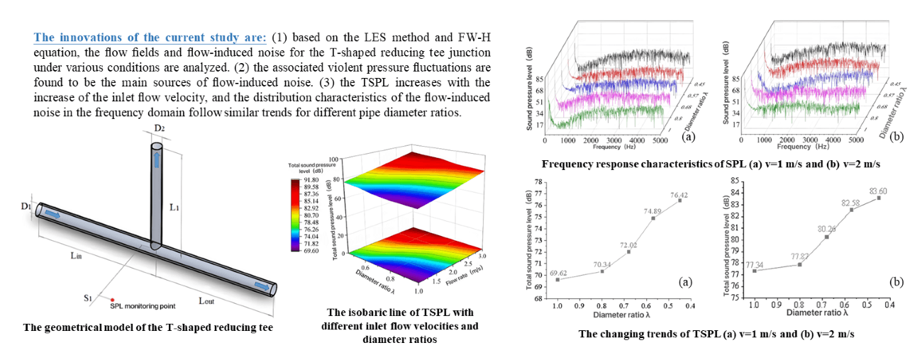
The so-called T-shaped reducing tees are typically used to divide, change and control (to a certain extent) the flow direction in pipe networks. In this study, the Ffowcs Williams–Hawkings (FW-H) equation and the Large Eddy Simulation (LES) methods are used to simulate the flow-induced noise related to T-shaped reducing tees under different inlet flow velocities and for different pipe diameter ratios. The results show that the maximum flow velocity, average flow velocity, and vorticity in the branch pipe increase gradually as the related diameter decreases. Strong vorticity and secondary flows are also observed in the branch pipe, and the associated violent pressure fluctuations are found to be the main sources of flow-induced noise. In particular, as the pipe diameter ratio decreases from 1 to 0.45, the Total Sound Pressure Level (TSPL) increases by 6.8, 6.26, and 7.43 dB for values of the inlet flow velocity of 1, 2, and 3 m/s, respectively. The distribution characteristics of the flow-induced noise in the frequency domain follow similar trends for different pipe diameter ratios.Graphic Abstract
Keywords
As an important part of the piping system, the T-shaped reducing tee junction is widely used in residential life and industrial production. When the fluid flows through the T-shaped reducing tee junction, the pressure and flow velocity change rapidly, causing the appearance of flow-induced noise. The noise of tee junction can damage the stability of the equipment and human health, so an in-depth study of the generation mechanism and noise characteristics is necessary.
Flow field characteristics are the basis of acoustic studies, and several researchers have performed a number of experiments and numerical simulations [1–3] on tee junctions. Beneš et al. [4] explored the laminar and turbulent flow characteristics of Newtonian and non-Newtonian fluids based on numerical simulation, and the results showed that the explicit algebraic Reynolds stress turbulence model [5] could capture the secondary flow in the branch pipe. Chen et al. [6] analyzed the influence of flow velocity, pipe diameter ratio and split ratio on the local loss coefficient of the tee. They revealed that the pipe diameter ratio had little effect on the loss coefficient in the branch pipe. Gao et al. [7] researched the air-conditioning duct tee through experiments and computational fluid dynamics (CFD) simulations, and proposed to reduce the turbulent energy dissipation and deformation by installing the guide vane.
In addition to the study of flow characteristics, some researchers have made significant contributions to the study of flow-induced noise of pipes [8]. Li et al. [9] used the Large Eddy Simulation (LES) method and Ffowcs Williams–Hawkings (FW-H) equation to simulate the noise induced by natural gas tee pipeline, and the aerodynamic noise [10] characteristics with different inlet and outlet combinations were obtained.
Han et al. [11] researched the flow-induced noise of natural gas manifolds by adopting LES and FW-H methods and obtained the best section area ratio of distribution pipe to outlet pipes for reducing noise. Mori et al. [12] studied flow-induced noise characteristics of T-shaped pipe with a square cross-section. The results showed that the aerodynamic sound pressure depends on the inlet velocity, while the flow velocity affects little on the directivity and frequency characteristics of the sound pressure.
According to the literature review, the studies on the tee junction focused on the flow velocity, local loss coefficient, split ratio, aerodynamic noise, etc. [13–15]. Furthermore, previous research mainly focused on the noise of the equal-diameter tee. However, little research discusses the flow-induced noise of reducing tees. Therefore, the flow and acoustic characteristics of the T-shaped reducing tee junction for variable pipe diameter ratios were investigated with numerical simulations in this research. The numerical simulation on the 3D flow field and flow-induced noise characteristics for the T-shaped reducing tee junction can guide the cooperative research of pipe selection and noise control.
2 Numerical Models and Methods
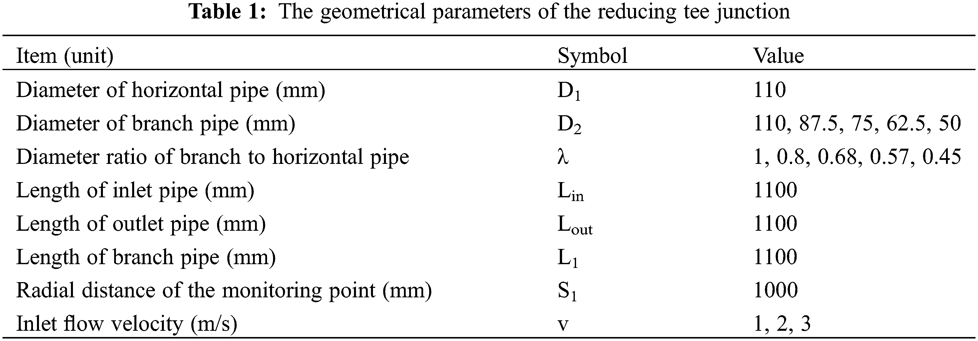
The geometrical model and parameters of the T-shaped reducing tee pipe are shown in Fig. 1 and Table 1, respectively. The horizontal pipe diameter (D1) is 110 mm, and the branch pipe diameter (D2) is 110, 87.5, 75, 62.5, and 50 mm, respectively. For convenience’s sake, this study uses the λ to represent D2/D1, and the pipe diameter ratio (λ) is 1, 0.8, 0.68, 0.57, and 0.45, respectively. In order to ensure the fluid flow in a fully developed, the pipe length of the inlet and outlet pipelines is ten times the size of the inlet diameter, respectively. To obtain the distribution characteristics of noise outside the pipe, the monitoring point S1 is set as shown in Fig. 1, and the radial distance of monitoring point S1 is 1000 mm.
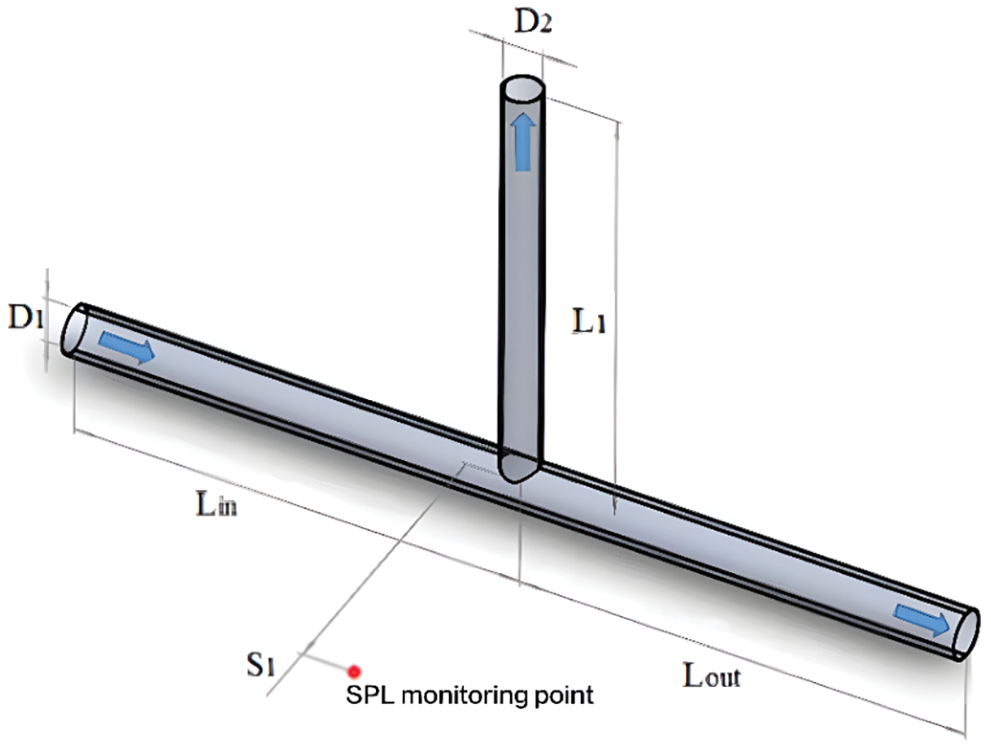
Figure 1: The geometrical model of the T-shaped reducing tee
In this research, using the water as the medium, and the flow in the T-shaped reducing tee can be considered as incompressible. Besides, the flow and noise characteristics under five different pipe diameter ratios and three different flow velocity conditions are discussed.
The LES model simulates the transient flow field [16–19]. In the LES, based on the eddy scale, the vortex is divided into two parts, namely large and small eddies. The N-S equations are filtered to establish the governing equations for LES in the physical space. The basic idea is to identify the cut-off scale with a filter function, and above the cut-off scale large eddies are calculated directly, below the cut-off scale the small eddies are closed with a numerical model [20,21], while the small-scale eddies are simulated with an appropriate sub-grid scale (SGS) model. The continuity equation and the N-S equation for filtration can be expressed as [22]
where
The Smagorinsky-Lilly model is used in the study, and the subgrid-scale stress
where
The commercial software ANASYS FLUENT is used to simulate the flow fields. The inlet boundary is defined as the velocity inlet, and the inner walls are set as the no-slip wall. The simulation results of steady flow fields are used as the initial condition for the simulation of transient flow fields. The PISO algorithm is ued to solve the pressure-velocity coupling equation. The time step is set as 10−4 s, and more than 10000 steps are used to calculate turbulent flows.
After the steady and transient flow field simulations, the FW-H method can calculate the flow-induced noise characteristics [23]. Based on the Fast Fourier Transform (FFT), the time-domain signal can be converted to the frequency-domain signal, then the frequency response characteristics of noise is obtained.
The FW-H acoustic model is based on Lighthill’s acoustic analogy theory. It properly describes the sound problem resulting from the interaction of fluids and moving objects. The key of this method is to transform the N-S equation into a non-homogeneous wave equation. The FW-H equation can be expressed as [24]
where
In the Eq. (4), the first term on the right side represents a quadrupole source caused by surface acceleration or displacement distribution; the second term represents a dipole acoustic source caused by surface pressure fluctuations; and the third term represents a monopole acoustic source caused by flow turbulence. The inner walls can be seen as completely rigid walls. Therefore, the diploe sources are considered for the noise calculation. In this study, the transient flow field is obtained based on the LES method and the flow-induced noise is calculated using the FW-H equation.
3.1 Grid Independence Analysis
The grid system with hexahedral elements is generated for the simulation of flow field. To obtain more accurate calculation results, the mesh for the near-wall region is refined and the height of the layer mesh is determined by [25]
where
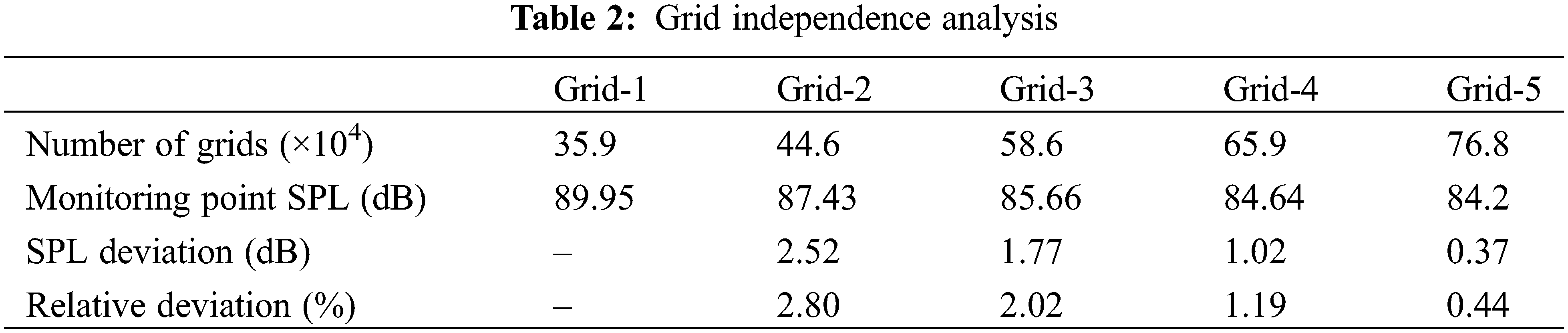
To conduct the grid independence analysis, the Sound Pressure Levels (SPL) at the monitoring point with five different grid systems are compared. As shown in Table 2, there is no obvious difference in the SPL for grid-5 compared with that obtained from grid-1 to grid-4. The results indicate that both grid-4 and grid-5 are suitable for numerical simulations, the grid is suitable for numerical simulation when the grid number is more than 6.59 × 10⁵. To improve the accuracy while reducing the computational costs, the grid-5 is adopted for the simulation in the following sections.
To confirm the feasibility of the numerical model, the frequency response characteristics of SPL and the Total Sound Pressure Level (TSPL) are calculated, and the results are compared with the experimental results of the previous research [26]. The structural diagram of the experimental model is shown in Fig. 2, and two monitoring points are set. Figs. 3a and 3b depict the comparison results of the frequency response characteristics of SPL obtained by simulation and experiment for monitoring points 1 and 2, respectively.

Figure 2: Structural diagram of the verification model

Figure 3: Comparison of SPL obtained by simulation and experiment at different monitoring points
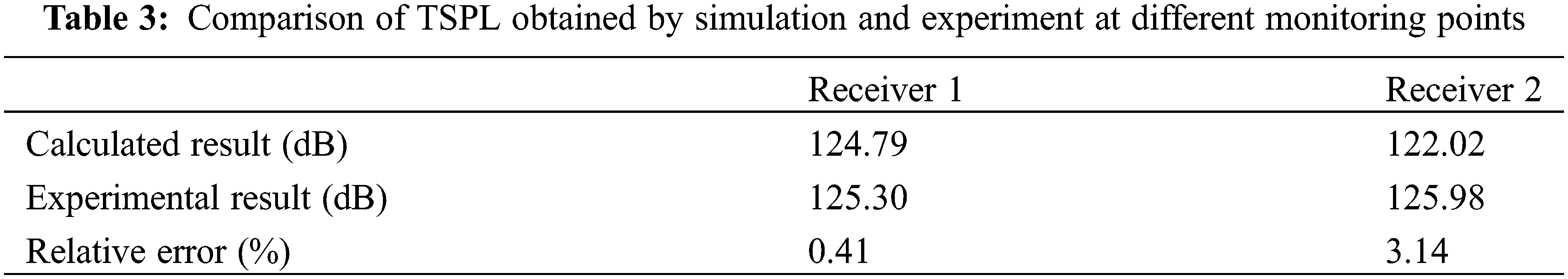
It can be seen that the changing trends of SPL obtained by simulation is similar to the results obtained by experiments. Additionally, the comparison of TSPL is listed in Table 3, the maximum value of relative error is 3.14%, and the average relative error is 1.78%. It can be concluded that the simulation method proposed in this study is reliable for the following work.
4 Simulation Results and Analysis
In order to analyze the influence of different pipe diameter ratios on the flow field and flow-induced noise, the distribution characteristics of pressure, velocity and vorticity with different velocities are analyzed.
4.1 The Distribution Characteristics of Flow Field with Different Pipe Diameter Ratios
When the inlet flow velocity is 3 m/s, the pressure distribution characteristics with different pipe diameter ratios are shown in Fig. 4. It can be found that the pipe diameter ratio has little effect on the pressure of inlet and outlet sections, while it mainly affects the pressure of the branch pipe. The low-pressure zone is located at the intersection of the main and branch pipe. As the pipe diameter ratio decreases, the average and minimum pressure of the branch pipe decrease gradually, and the low-pressure zone moves downstream of the branch pipe. When the pipe diameter ratio decreases from 1 to 0.45, the average pressure of the branch pipe decreases from −2303 to −45217 Pa, respectively, and the minimum pressure decreases from −8058 to −72427 Pa, respectively.
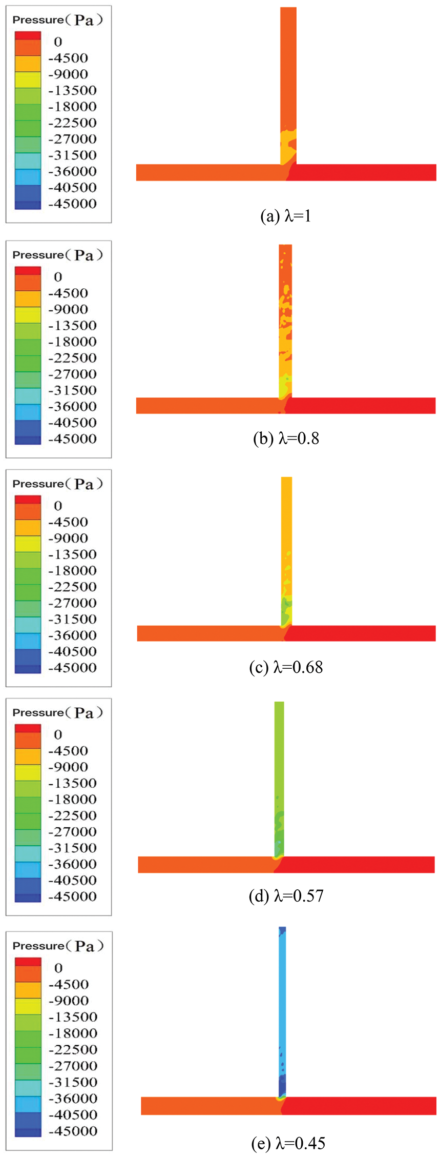
Figure 4: The pressure distribution characteristics for different pipe diameter ratios at v = 3 m/s
The velocity distribution characteristics with different pipe diameter ratios under 3 m/s are shown in Fig. 5. The pipe diameter ratio has little effect on the average flow velocity at the horizontal pipe outlet section, while it mainly affects the flow velocity in the branch pipe. When the pipe diameter ratio decreases from 1 to 0.45, there is a low-velocity zone on the side of the branch pipe wall close to the inlet. Besides, strong vortex and secondary flow appear in the low-velocity zone. There is an obvious dividing line between the high-velocity and low-velocity zones. As the pipe diameter ratio decreases, the average flow velocity in the branch pipe increases from 1.52 to 7.27 m/s, respectively, and the maximum flow velocity increases from 5.46 to 11.28 m/s, respectively.
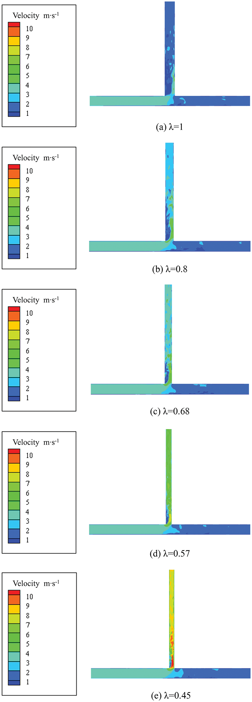
Figure 5: The velocity distribution characteristics for different pipe diameter ratios at v = 3 m/s
As shown in Figs. 6 and 7, the flow characteristics with three inlet flow velocities and five pipe diameter ratios are compared. When the inlet flow velocity is constant, the average and minimum pressure in the branch pipe decrease with the increase of the pipe diameter ratio. The smaller the pipe diameter ratio is, the greater the average and minimum pressure drop is. When the pipe diameter ratio keeps unchanged, the average and minimum pressure in the branch pipe decrease with the increase of the inlet flow, when the pipe diameter ratio decreases from 1 to 0.45, the average pressure in the branch pipe with the inlet flow velocity of (1, 2, and 3 m/s) decreases by 4943, 19182, and 42914 Pa, respectively, the minimum pressure decreases by 7670, 29849, and 64369 Pa, respectively. Therefore, when the pipe diameter ratio decreases, the average and minimum pressure drop increases with the increase of flow velocity.
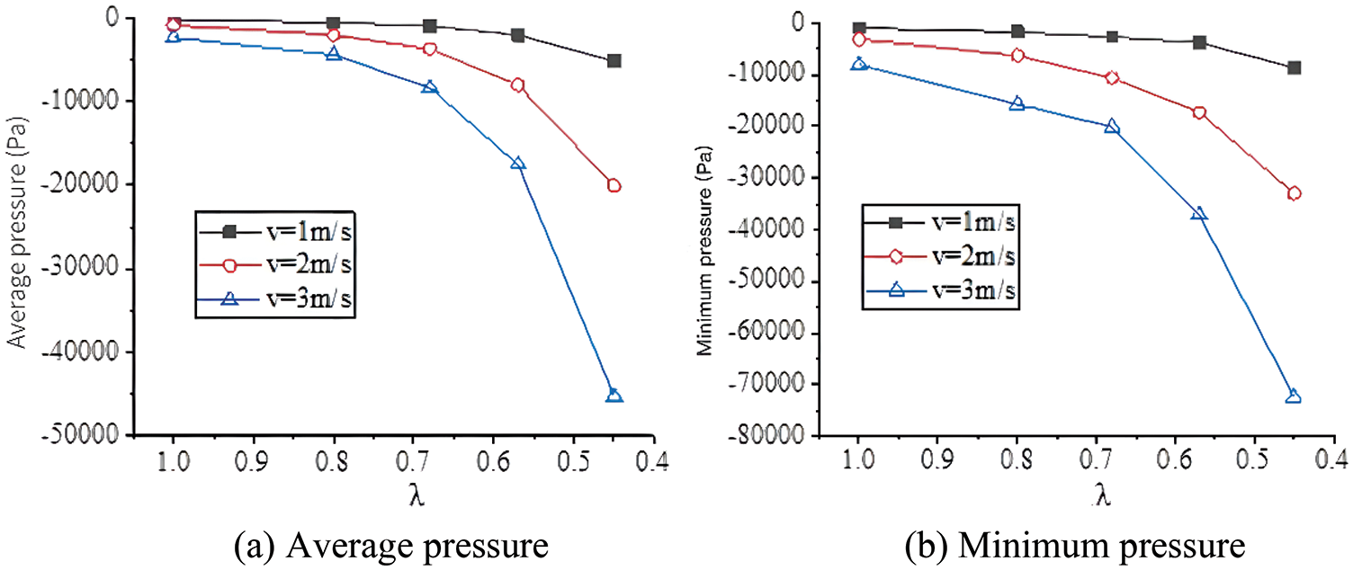
Figure 6: The changing trends of pressure under various conditions
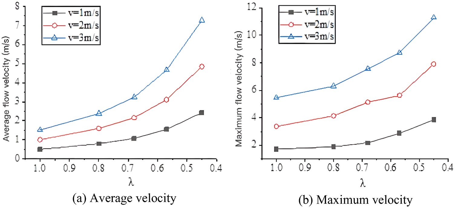
Figure 7: The changing trends of velocity under various conditions
The average and maximum flow velocity in the branch pipe increases with the increase of inlet flow velocity and the decrease of pipe diameter ratio. When the diameter ratio decreases from 1 to 0.45, the average flow velocity in the branch pipe with the inlet flow velocity of (1, 2, and 3 m/s) increases by 1.93, 3.84, and 5.75 m/s, respectively, and the maximum flow velocity in the branch pipe increases by 2.21, 4.54, and 5.82 m/s, respectively. When the pipe diameter ratio is constant, the greater the inlet flow velocity is, the greater the increase of the average and maximum velocity in the branch pipe is.
Fig. 8 shows the vorticity distribution characteristics in T-shaped reducing tee with different diameter ratios under 3 m/s. When the pipe diameter ratio is 1, the local maximum vorticity is 2473 s−1, which is located downstream of the recirculation and accelerating zone. When the pipe diameter ratio is 0.8 and 0.68, the maximum vorticity is 3663 and 4963 s−1, respectively. When the diameter ratio decreases to 0.57 and 0.45, the maximum vorticity increases to 8450 and 17071 s−1, respectively. In addition, the vorticity increases downstream of the recirculation and accelerating zone, and the influence distance of the vortex increases downstream of the accelerating zone.
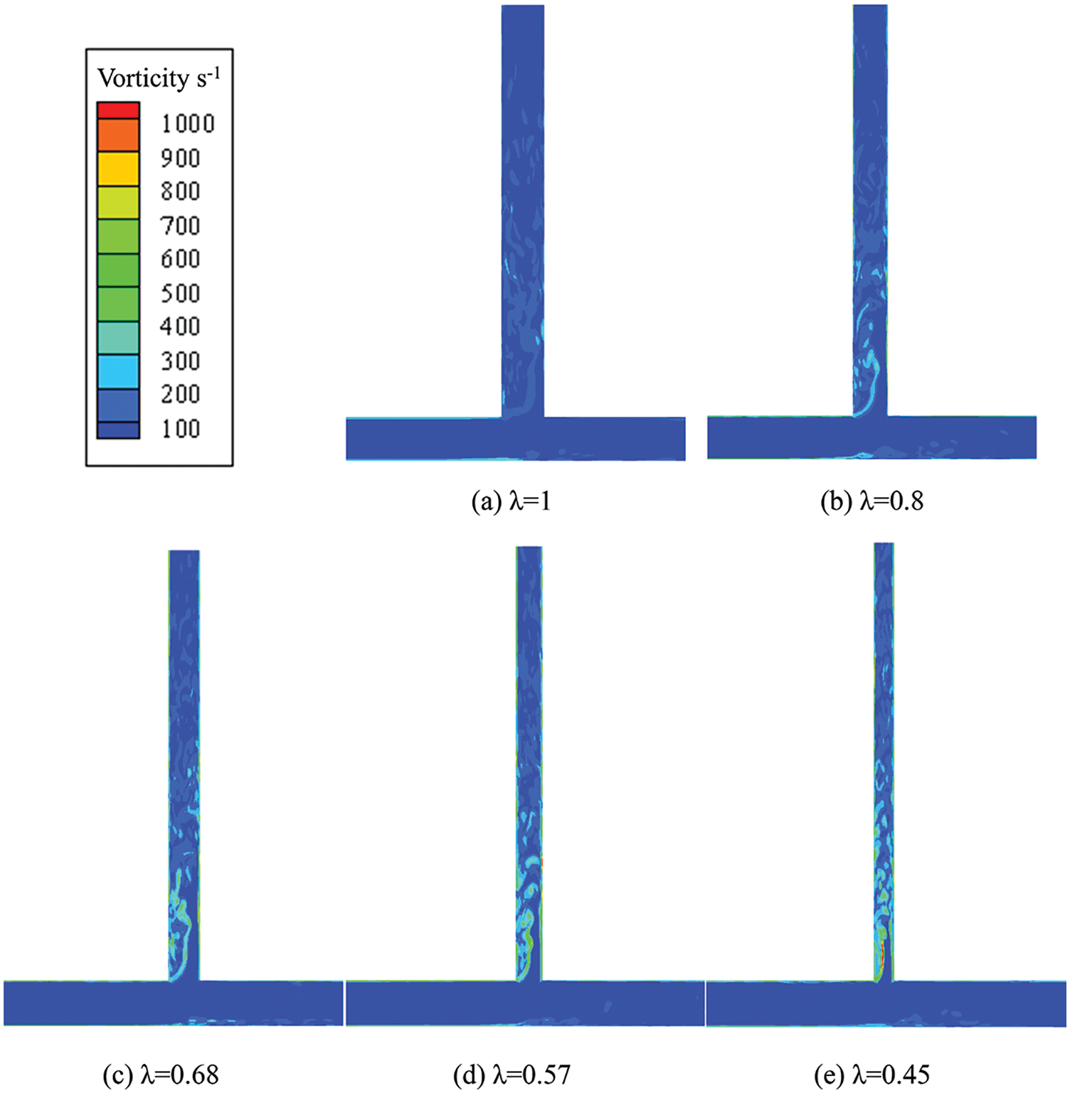
Figure 8: The distribution characteristics of vorticity with different pipe diameter ratios at v = 3 m/s
In addition, the pipe diameter ratio affects little on the vorticity in the main pipe, while it has a greater effect on the vorticity in the branch pipe. With decreasing the pipe diameter ratio, the vorticity in the branch pipe increases gradually. The vortex obviously increases in the recirculation zone and its downstream zone, and the development distance of the vortex in the downstream of the branch pipe also increases significantly.
4.2 The Flow-Induced Noise Characteristics with Different Diameter Ratios
The SPL spectra can be obtained by using FFT on the time-domain signal, then TSPL can be calculated as follows:
where
Fig. 9 presents the changing trends of flow-induced noise with different pipe diameter ratios under 1 m/s. It is observed that the frequency response characteristics of noise changes slightly with different pipe diameter ratios, specifically, the SPL in the range of 0–200 Hz is much higher than that in other ranges, while the minimum SPL appears in the frequency range of 300–400 Hz, then the SPL presents the fluctuation characteristics in the high-frequency range. As the pipe diameter ratio decreases, the SPL is in the range of 500–3000 Hz increases apparently. Moreover, the TSPL increases gradually with the decrease of pipe diameter ratio. When the pipe diameter ratio decreases from 1 to 0.45, the TSPL increases by about 9.77%.
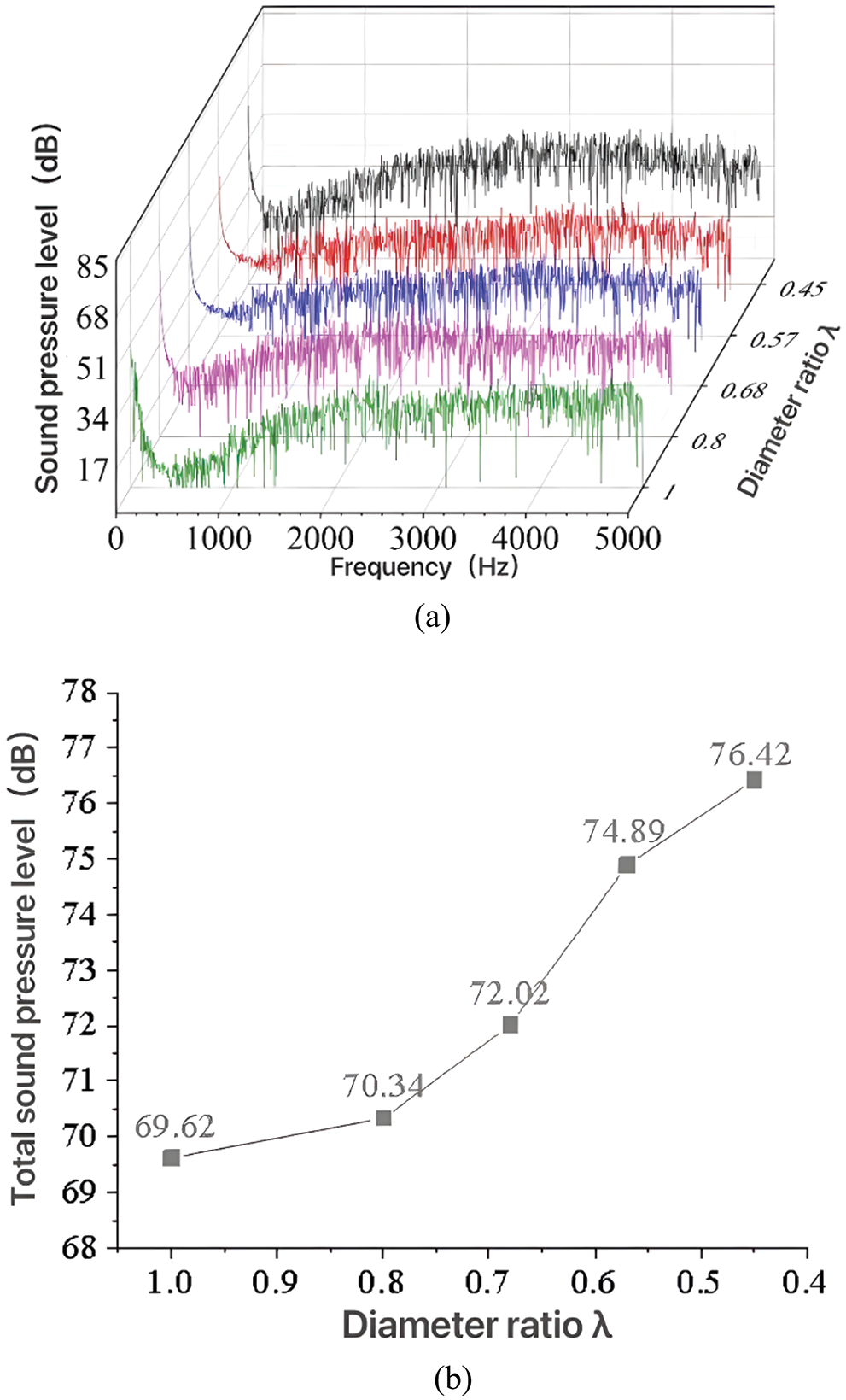
Figure 9: The changing trends of flow-induced noise with different pipe diameter ratios at v = 1 m/s. (a) Frequency response characteristics of SPL, (b) The changing trends of TSPL
The frequency characteristics of flow-induced noise with different diameter ratios under 2 m/s are shown in Fig. 10. It is observed that the frequency response characteristics of noise changes slightly with different pipe diameter ratios specifically, the SPL in the range of 0–200 Hz is much higher than that in other ranges. As the pipe diameter ratio decreases, the SPL is in the range of 1000–4500 Hz increases apparently. Moreover, the TSPL increases gradually with the decrease of pipe diameter ratio. When the pipe diameter ratio decreases from 1 to 0.45, the TSPL increases by about 8.09%.
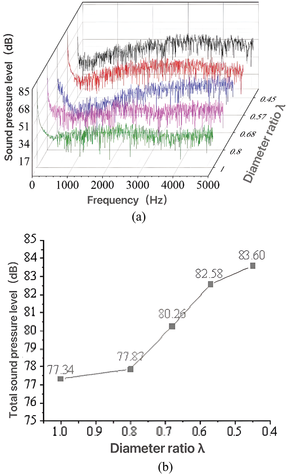
Figure 10: The changing trends of flow-induced noise with different pipe diameter ratios at v = 2 m/s. (a) Frequency response characteristics of SPL, (b) The changing trends of TSPL
Fig. 11 illustrates the changing trends of flow-induced noise at different pipe diameter ratios under 3 m/s. Similar to the distribution characteristics of noise under 1 and 2 m/s, the maximum value of SPL appears in the range from 0 to 200 Hz. However, the change of pipe diameter ratio affects the SPL in the high-frequency range significantly. As the pipe diameter ratio decreases, the SPL is in the range of 2500–5000 Hz increases apparently. Moreover, the TSPL increases with the decrease of pipe diameter ratio. When the pipe diameter ratio decreases from 1 to 0.45, the TSPL increases by about 8.82%.
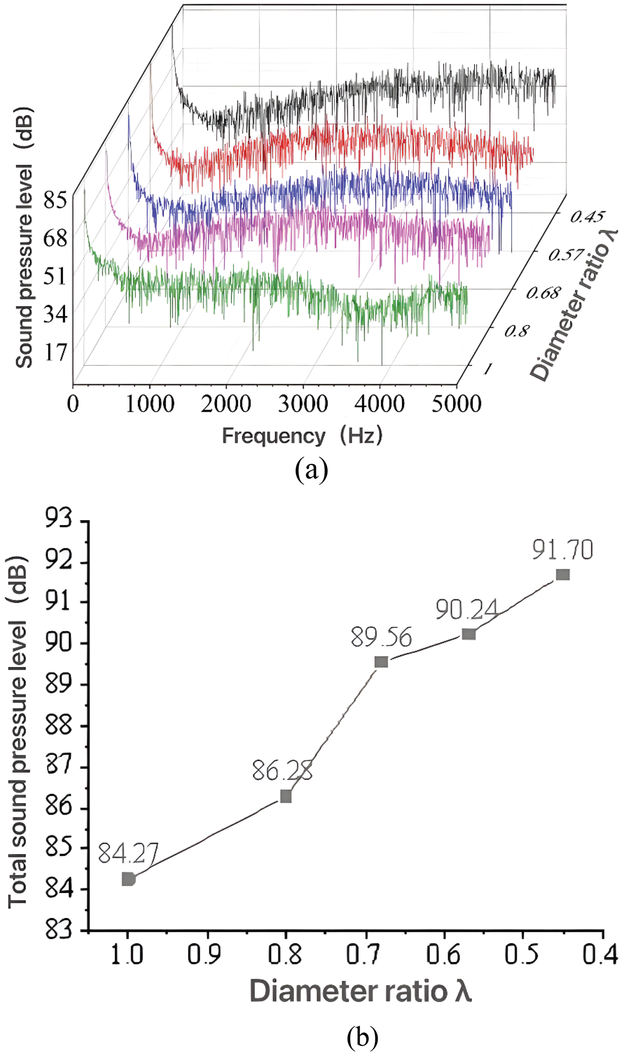
Figure 11: The changing trends of flow-induced noise with different pipe diameter ratios at v = 3 m/s. (a) Frequency response characteristics of SPL, (b) The changing trends of TSPL
Fig. 12 shows the isobaric line of TSPL with different inlet flow velocities and pipe diameter ratios. It can roughly predict the flow-induced noise level of T-shaped reducing tee under different working conditions. The inlet flow velocity and pipe diameter ratio have great influence on the flow-induced noise of the T-shaped reducing tee. The TSPL increases with the increase of inlet flow velocity and the decrease of pipe diameter ratio.

Figure 12: The isobaric line of TSPL with different inlet flow velocities and diameter ratios
4.3 Prediction of the Flow-Induced Noise
Since the TSPL of T-shaped reducing tee is mainly affected by the inlet flow velocity and pipe diameter ratio [27]. And to further predict the flow-induced noise characteristics of T-shaped reducing tee, the TSPL with different flow velocities and pipe diameter ratios are calculated, which is shown in Table 4.
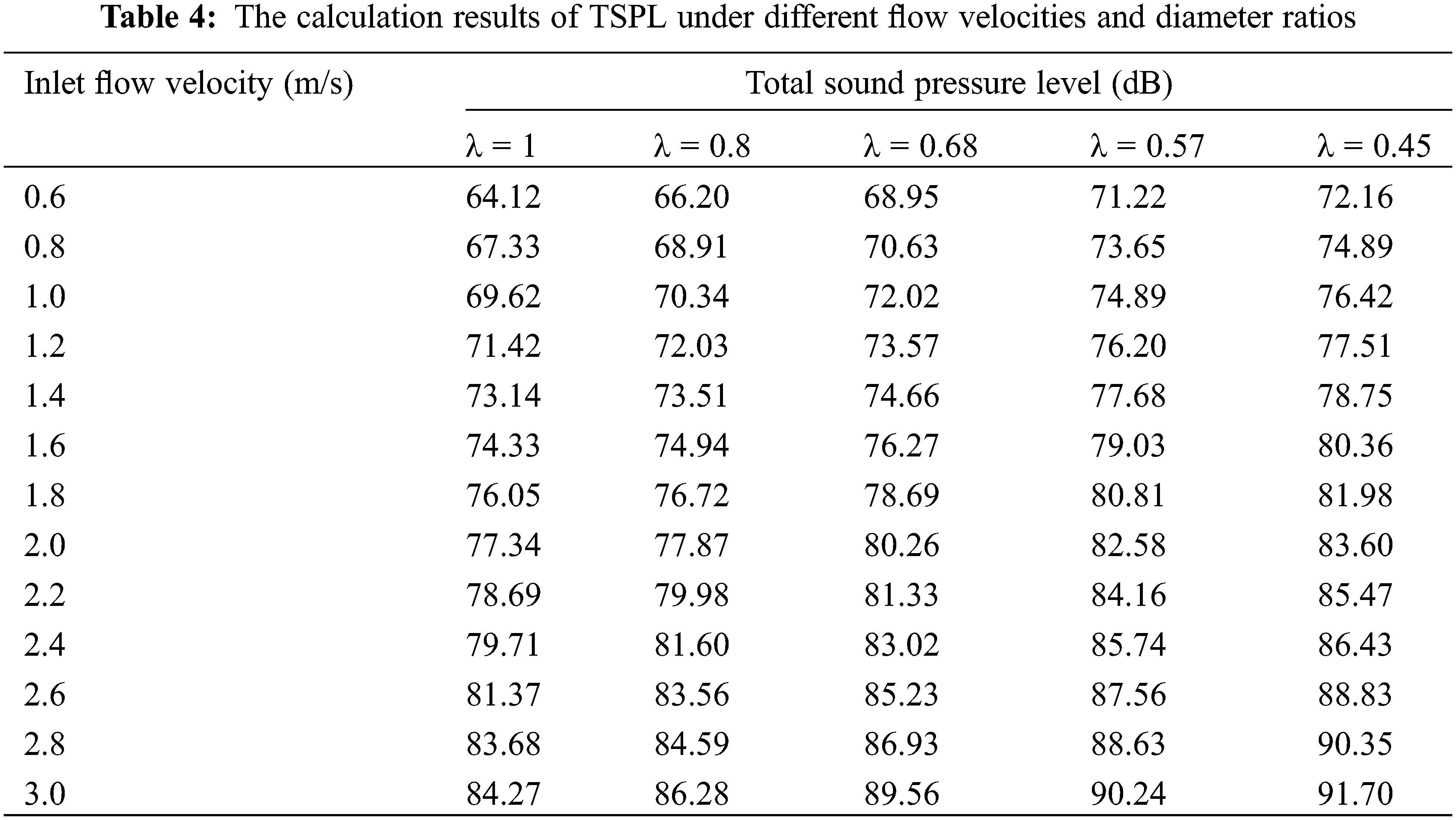
It is found from Table 4 that the TSPL has a linear relationship with the inlet velocity V and the pipe diameter ratio
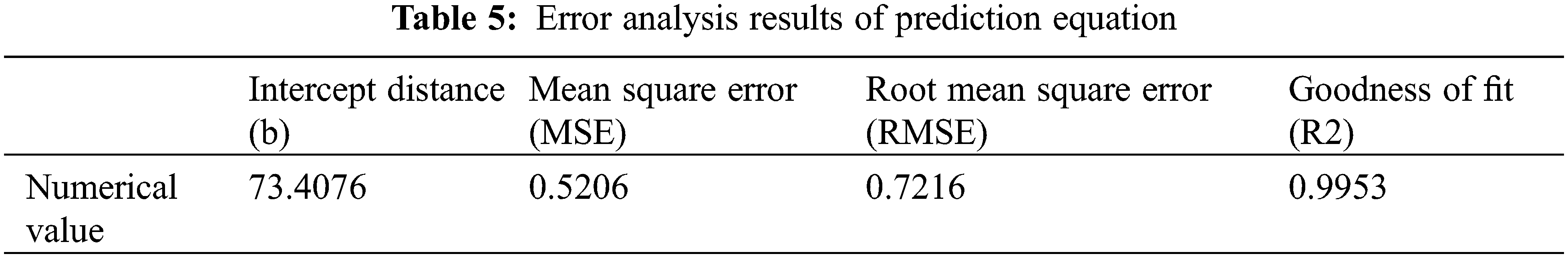
The error analysis results are listed in Table 5. As can be seen, the RMSE is only 0.7216 and the goodness of fit is 0.9953, which means that the Eq. (9) can predict the flow-induced noise of the T-shaped reducing tee accurately.
Based on the LES method and FW-H equation, the flow fields and flow-induced noise for the T-shaped reducing tee junction under various conditions are analyzed. The main conclusions are as follows:
(1) Under the influence of the pipe diameter ratio, the maximum flow velocity and average flow velocity in the branch pipe increase gradually as the related diameter decreases.
(2) Strong vorticity and secondary flows are observed in the branch pipe. As the diameter ratio decreases, the vorticity of the reflux zone and its downstream in the branch pipe gradually increases. Concurrently, the influence distance of the vortex in the downstream of the reflux area increases significantly.
(3) The associated violent pressure fluctuations are found to be the main sources of flow-induced noise. The TSPL increases with the increase of the inlet flow velocity, and the distribution characteristics of the flow-induced noise in the frequency domain follow similar trends for different pipe diameter ratios.
Funding Statement: This study is supported by the Shandong Engineering Laboratory for High-Efficiency Energy Conservation and Energy Storage Technology & Equipment.
Conflicts of Interest: The authors declare they have no conflicts of interest, financial or non-financial.
References
1. Yin, Y. T., Chen, K., Qiao, X. Y., Lin, M., Lin, Z. M. et al. (2017). Mean pressure distributions on the vanes and flow loss in the branch in a T pipe junction with different angles. Energy Procedia, 105(12), 3239–3244. DOI 10.1016/j.egypro.2017.03.718. [Google Scholar] [CrossRef]
2. Guo, C., Gao, M. (2020). Investigation on the flow-induced noise propagation mechanism of centrifugal pump based on flow and sound fields synergy concept. Physics of Fluids, 32(3), 035115. DOI 10.1063/5.0003937. [Google Scholar] [CrossRef]
3. Rao, A. R., Padmavathi, K. (1993). Pulsatile flow of a viscous fluid in elliptical pipe of variable cross-section. International Journal of Non-Linear Mechanics, 28(4), 455–466. DOI 10.1016/0020-7462(93)90019-H. [Google Scholar] [CrossRef]
4. Beneš, L., Louda, P., Kozel, K., Keslerová, R., Štigler, J. (2013). Numerical simulations of flow through channels with T-junction. Applied Mathematics and Computation, 219(13), 7225–7235. DOI 10.1016/j.amc.2011.04.074. [Google Scholar] [CrossRef]
5. Wallin, S., Johansson, A. (2000). An explicit algebraic Reynolds stress model for incompressible and compressible turbulent flows. Journal of Fluid Mechanics, 403, 89–132. DOI 10.1017/S0022112099007004. [Google Scholar] [CrossRef]
6. Chen, J. L., Lv, H. X., Shi, X., Zhu, D. L., Wang, W. E. (2012). Numerical simulation and experimental study on hydrodynamic characteristics of T-type pipes. Transactions of the Chinese Society of Agricultural Engineering, 28(5), 73–77. [Google Scholar]
7. Gao, R., Liu, K. K., Li, A. G., Fang, Z. Y., Yang, Z. G. et al. (2018). Study of the shape optimization of a tee guide vane in a ventilation and air-conditioning duct. Building and Environment, 132(3), 345–356. DOI 10.1016/j.buildenv.2018.02.006. [Google Scholar] [CrossRef]
8. Hambric, S. A., Boger, D. A., Fahnline, J. B., Campbell, R. L. (2010). Structure- and fluid-borne acoustic power sources induced by turbulent flow in 90° piping elbows. Journal of Fluids and Structures, 26(1), 121–147. DOI 10.1016/j.jfluidstructs.2009.10.001. [Google Scholar] [CrossRef]
9. Li, C. J., Yan, S. K., Wen, D. D., Huang, Q., Lin, Y. (2018). CFD analysis of flow noise at tees at natural gas station. Noise Control Engineering Journal, 66(1), 1–10. DOI 10.3397/1/37661. [Google Scholar] [CrossRef]
10. Weinmann, M., Sandberg, R. D., Doolan, C. (2014). Tandem cylinder flow and noise predictions using a hybrid RANS/LES approach. International Journal of Heat and Fluid Flow, 50(4), 263–278. DOI 10.1016/j.ijheatfluidflow.2014.08.011. [Google Scholar] [CrossRef]
11. Han, T., Wang, L., Cen, K., Song, B., Shen, R. Q. et al. (2020). Flow-induced noise analysis for natural gas manifolds using LES and FW-H hybrid method. Applied Acoustics, 159(10), 107101. DOI 10.1016/j.apacoust.2019.107101. [Google Scholar] [CrossRef]
12. Mori, M., Masumoto, T., Ishihara, K. (2017). Study on acoustic and flow induced noise characteristics of T-shaped pipe with square cross-section. Advances in Applied, 120(5), 137–147. DOI 10.1016/j.apacoust.2017.01.022. [Google Scholar] [CrossRef]
13. Aladwani, A., Almandeel, A., Nouh, M. (2019). Fluid-structural coupling in metamaterial plates for vibration and noise mitigation in acoustic cavities. International Journal of Mechanical Sciences, 152(5), 151–166. DOI 10.1016/j.ijmecsci.2018.12.048. [Google Scholar] [CrossRef]
14. Kojima, T., Inaba, K. (2020). Numerical analysis of wave propagation across solid-fluid interface with fluid-structure interaction in circular tube. International Journal of Pressure Vessels and Piping, 183, 104099. DOI 10.1016/j.ijpvp.2020.104099. [Google Scholar] [CrossRef]
15. Li, A. G., Chen, X., Chen, L., Gao, R. (2014). Study on local drag reduction effects of wedge-shaped components in elbow and T-junction close-coupled pipes. Building Simulation, 7(2), 175–184. DOI 10.1007/s12273-013-0113-z. [Google Scholar] [CrossRef]
16. Liu, E. B., Yan, S. K., Wang, D., Huang, L. Y. (2015). Large eddy simulation and FW-H acoustic analogy of flow-induced noise in elbow pipe. Journal of Computational and Theoretical Nanoscience, 12(9), 2866–2873. DOI 10.1166/jctn.2015.4191. [Google Scholar] [CrossRef]
17. Itoh, Y., Tamura, T. (2008). Large eddy simulation of turbulent flows around bluff bodies in overlaid grid systems. Journal of Wind Engineering and Industrial Aerodynamics, 96(10–11), 1938–1946. DOI 10.1016/j.jweia.2008.02.065. [Google Scholar] [CrossRef]
18. Es-Sahil, O., Sescu, A., Afsar, M. Z., Buxton, O. R. (2020). Investigation of wakes generated by fractal plates in the compressible flow regime using large-eddy simulations. Physics of Fluids, 32(10), 105106. DOI 10.1063/5.0018712. [Google Scholar] [CrossRef]
19. Queguineur, M., Bridel-Bertomeu, T., Gicquel, L. Y., Staffelbach, G. (2019). Large eddy simulations and global stability analyses of an annular and cylindrical rotor/stator cavity limit cycles. Physics of Fluids, 31(10), 104109. DOI 10.1063/1.5118322. [Google Scholar] [CrossRef]
20. Cheng, H. Y., Bai, X. R., Long, X. P., Ji, B., Peng, X. X. et al. (2020). Large eddy simulation of the tip-leakage cavitating flow with an insight on how cavitation influences vorticity and turbulence. Applied Mathematical Modelling, 77(1), 788–809. DOI 10.1016/j.apm.2019.08.005. [Google Scholar] [CrossRef]
21. Li, Z. W., Huai, W. X., Han, J. (2011). Large eddy simulation of the interaction between wall jet and offset jet. Journal of Hydrodynamics, 23(5), 544–553. DOI 10.1016/S1001-6058(10)60148-5. [Google Scholar] [CrossRef]
22. Zhang, Y. O., Zhang, T., Ouyang, T., Li, Y. (2014). Flow-induced noise analysis for 3D trash rack based on LES/Lighthill hybrid method. Applied Acoustics, 79, 141–152. DOI 10.1016/j.apacoust.2013.12.016. [Google Scholar] [CrossRef]
23. Kim, H., Lee, S., Son, E., Lee, S., Lee, S. (2012). Aerodynamic noise analysis of large horizontal axis wind turbines considering fluid-structure interaction. Renewable Energy, 42, 46–53. DOI 10.1016/j.renene.2011.09.019. [Google Scholar] [CrossRef]
24. Williams, J. E., Hawkings, D. L. (1969). Sound generation by turbulence and surfaces in arbitrary motion. Philosophical Transactions of the Royal Society of London Series A–Mathematical and Physical Sciences, 264, 321–342. [Google Scholar]
25. Jiang, J. W., Wang, W. Q., Chen, K., Huang, W. X. (2022). Large-eddy simulation of three-dimensional aerofoil tip-gap flow. Ocean Engineering, 243(2), 110315. DOI 10.1016/j.oceaneng.2021.110315. [Google Scholar] [CrossRef]
26. Lv, J., Ji, X. (2010). Study on prediction and experimental measurment of flow noise in pipes with variable cross-section area. Noise and Vibration Control, 31, 166–167. [Google Scholar]
27. Shi, J. W., Ge, S., Sheng, X. Z. (2022). Numerical investigation on the aerodynamic noise generated by a simplified double-strip pantograph. Fluid Dynamics & Materials Processing, 18(2), 463–480. DOI 10.32604/fdmp.2022.017508. [Google Scholar] [CrossRef]
Cite This Article
 Copyright © 2023 The Author(s). Published by Tech Science Press.
This work is licensed under a Creative Commons Attribution 4.0 International License , which permits unrestricted use, distribution, and reproduction in any medium, provided the original work is properly cited.
 Downloads
 Citation Tools