
 Submit a Paper
 Propose a Special lssue
 Open Access
ARTICLE

Computational Analysis of Surface Pressure Distribution over a 2D Wedge in the Supersonic and Hypersonic Flow Regimes
1 MIT School of Engineering, MIT ADT University, Pune, 412201, India
2 Trinity College of Engineering and Research, Pune, 411048, India
3 Department of Mechanical Engineering, International Islamic University Malaysia, Kuala Lumpur, 53100, Malaysia
* Corresponding Author: Javed S. Shaikh. Email:
Fluid Dynamics & Materials Processing 2023, 19(6), 1637-1653. https://doi.org/10.32604/fdmp.2023.025113
Received 23 June 2022; Accepted 27 September 2022; Issue published 30 January 2023
 View Full Text
 Download PDF
Abstract
The complex fluid-dynamic instabilities and shock waves occurring along the surface of a two-dimensional wedge at high values of the Mach number are studied here through numerical solution of the governing equations. Moreover, a regression model is implemented to determine the pressure distribution for various Mach numbers and angles of incidence. The Mach number spans the interval from 1.5 to 12. The wedge angles (θ) are from 5° to 25°. The pressure ratio (P2/P1) is reported at various locations (x/L) along the 2D wedge. The results of the numerical simulations are compared with the regression model showing good agreement.Keywords
Nomenclature
| Mp | Piston Mach number |
| M∞ | Freestream Mach number |
| α | angle of attack |
| q | pitch rate |
| a∞ | freestream velocity |
| P2 | pressure on the windward surface |
| P1 | freestream pressure |
| γ | specific heat ratio of the gas |
| M | Mach number |
| θ | angle of incidence |
| L | x/L ratio |
| u | instantaneous velocity |
| V | velocity modulus |
| ρ | gas density |
| P | gas pressure |
| qj | heat flux |
| τij | viscous stress tensor |
In space investigation, supersonic/hypersonic study is an absolute requisite and vital part. Tsien [1] revealed the concept similarity rule for irrotational and unsteady hypersonic flow. The outcome derived by him shows a good concurrence with the experimental results. Over a thin aerofoil, Hayes [2] studied the unsteady flow with high Mach numbers. The potential theory has been used to study unsteady supersonic flows. Zartarian et al. [3] have studied the unsteady hypersonic flow using the tangent-wedge approximation method and shock expansion theory. Carrier [4] gave the exact solution of an oscillating wedge for two-dimensional flow. Hui [5] derived a solution that is consistently applied for all supersonic Mach numbers and wedge angles in the case of an attached shock wave for an oscillating flat plate with a two-dimensional flow. Hui et al. [6] theory continued by Lui et al. [7] in pitch with an attached shock in the delta wing. Piston theory forecasts surface pressure on wings and panels in high-speed flows. Lighthill [8] originally developed the piston theory at a large scale of Mach number for the oscillating airfoils. Lighthill [8] introduces the term “Piston Analogy” by connecting the two-dimensional unsteady problem with the gas flow in a tube driven by a piston. Ghosh et al. [9] combined the piston theory of Lighthill [8] and shock expansion theory Mile’s [10] for the concept of order Ø2, where Ø the angle between the plane approximates the windward surface and the shock with the case of attached shock. Ghosh [11] evolved the similitude in the case of oscillating delta wings at hypersonic Mach number with high incidence for attached shock. Crasta et al. [12] have studied the variation in surface pressure distribution with the angle of incidence and Mach numbers for supersonic and hypersonic flow with a curved leading edge for the delta wing. The computational and analytical investigation of aerodynamic derivatives in the case of the oscillating Wedge is being studied by Musavir et al. [13]. Khan et al. [14] have revealed the CFD simulation with analytical and theoretical validation of different flow parameters for the Wedge at supersonic Mach number. Kalimuthu et al. [15] studied and measured aerodynamic coefficients at Mach 6 for the blunt body in consideration of without and with a spike. The trailing edge geometry effect on the aerodynamics of low-speed BWB aerial vehicles has been studied by Zuhair et al. [16]. Meng et al. [17] referred to the study of a double-cone missile by the combined spike and multi-jet. The analytical and computational analysis of pressure at the nose of a 2D wedge has been studied by Shaikh et al. [18].
In the present analysis, the main objective is to obtain the pressure distribution along the edge of the two-dimensional Wedge. Based on the CFD results, the regression model has been developed. The CFD analysis results of pressure with various Mach numbers and wedge angles are compared with the regression model for different flow parameters for the 2D planar Wedge. The CFD analysis is used together with a parametric study using ANSYS. The scale of Mach number is from 1.5 to 12, and the range of the wedge angle (θ) is from angles 5° to degree 25°. The geometry of plane wedge transfer of pivot position is shown in Fig. 1.
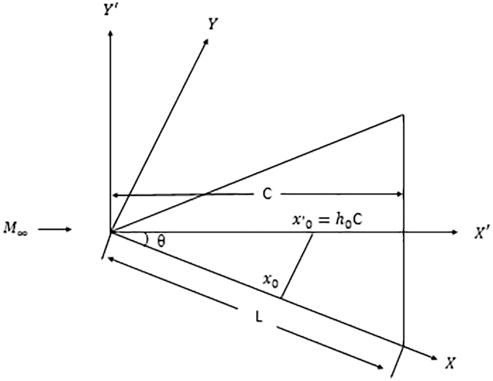
Figure 1: Geometry of plane wedge transfer of pivot position from x0 to x’0
Let the flat plate aerofoil of length (L) with the wedge angle (θ) oscillate with a minimal amplitude about the pivot position in pitch. The x0 is the distance from the apex. At any instant, the piston velocity at a distance x with the angle of attack α is given by Eq. (1),
The piston Mach number is given by Eq. (2),
The exact isentropic expression for the pressure on a piston as in the power series with its velocity to link the piston velocity and pressure on the piston surface was explored by Lighthill [8]. To fulfill the isentropic condition, the piston velocity is less than or equal to the free stream sound velocity condition. This theory is consistent with the theory of small disturbance on which the Lighthill [8] Piston theory is based.
As in the z-direction, the velocity component is minimum; then, along the z-direction, the strip of the wedge parallel to the centerline can be considered independent. That was revealed by Ghosh [11]. It merges the strip theory with the notable incidence similitude of Ghosh [11], resulting in ‘Piston analogy’, and it directly connects with the corresponding Mach number ‘MP’. In the present case, the piston Mach number and angle of incidence are admissible to a large extent. Thus, Lighthill’s [8] piston theory or strong shock expansion theory of Mile’s [10] is not used, but Ghosh piston theory is applied. The surface pressure P can directly give rise to inertia level at the piston on the wing’s surface. The pressure distribution expression is given by Eq. (3),
where,
Strips are assumed to be separate from each other at different span locations. The angle of the Wedge is the same as that of the wing. In different span locations, strips are considered separate from each other. The wedge angle is the same as that of the wing. In the present situation, both ‘Mp’ and flow deflection are allowed to be high.
Pathan et al. [19] have studied the boat tail helmets to reduce drag and found that the aerodynamic drag reduces when the helmet shape is streamlined. At Mach 1.5, the experimental research of wall pressure distribution and the effect of the microjet was revealed by Azami et al. [20]. Pathan et al. [21] the base pressure variation in external and internal flows using CFD analysis and found that the flow field in the base region of internal and external suddenly expanded flows are almost the same. Khan et al. [22] revealed that the microjets could work as active base pressure controllers. Pathan et al. [23–26] and Khan et al. [27] have studied various methods to control base pressure.
Based on the literature, it has been found that the pressure variation along the length of the Wedge has not been studied. In the present research work, the variation of the pressure along the edge at a combination of parameters has been studied.
The Computational Fluid Dynamics (CFD) was adopted for the analysis using Academic licensed ANSYS Workbench and Fluent. The modeling and meshing are completed in the ANSYS workbench, and the Fluent is used for analysis. The range of Mach numbers 1.5, 2.0, 2.5, 3.0, 3.5, 4.0, 6.0, 8.0, 10.0, and 12.0 are taken into consideration for the analysis along with the wedge angles 5°, 10°, 15°, 20° and 25°. All possible combinations of parameters are used for CFD analysis for the weak solutions where the shockwave is attached [28]. For the CFD analysis, air as ideal gas is considered a fluid. Fig. 2 shows the boundary conditions used for CFD analysis.
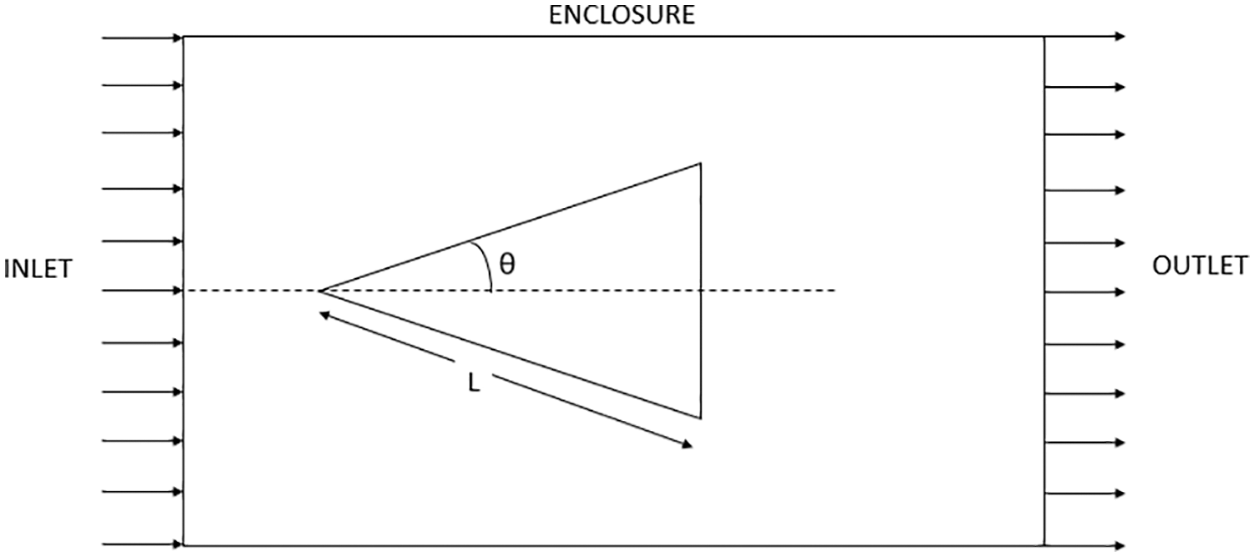
Figure 2: Geometry of 2D Wedge and enclosure for CFD analysis
The ANSYS design modeler is used for modeling all geometries by varying the wedge angle. The geometry of the 2D Wedge and enclosure are shown in Fig. 2. All the geometries are modeled by considering the range of wedge angle (θ) from 5° to 25°. The length (L) = 10 mm for all the geometry is considered. For the CFD analysis, the enclosure is created with three times the length (L) front side, five times the length (L) on the rear side, and five times the length (L) on the top and bottom sides. The inlet and outlet names are given to the front and rear edges, as shown in Fig. 2
The grid independence test is performed before proceeding with the meshing to find the optimum size of the mesh elements. The grid independence test was done for wedge angle 10° and Mach number 1.5 by varying mesh size from 1 to 40 mm. Table 1 shows the number of elements and nodes for mesh sizes from 40 to 1 mm.
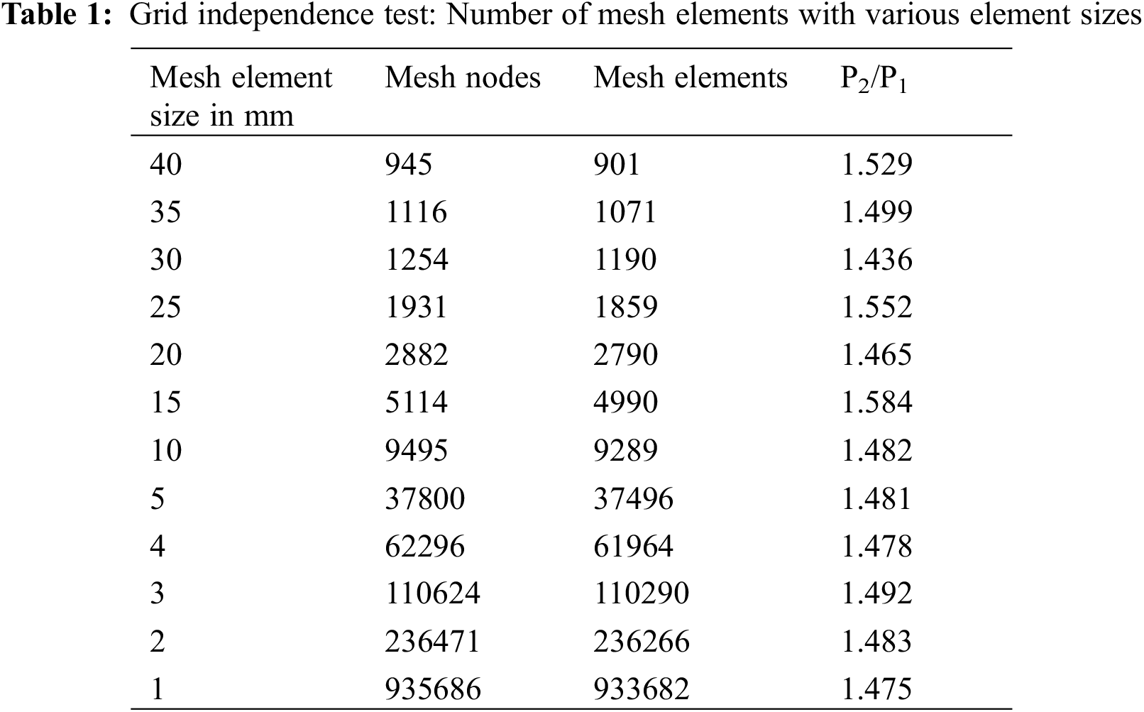
Table 1 shows the results of the grid independence test. The results show that the change in the results is negligible at 10 mm of the mesh element size. The 10 mm mesh element size can be considered for further CFD analysis. Fig. 3a reveals the entire meshed model and the expanded view of the wedge geometry shown in Fig. 3b. The Hexahedral mesh elements are considered for meshing.
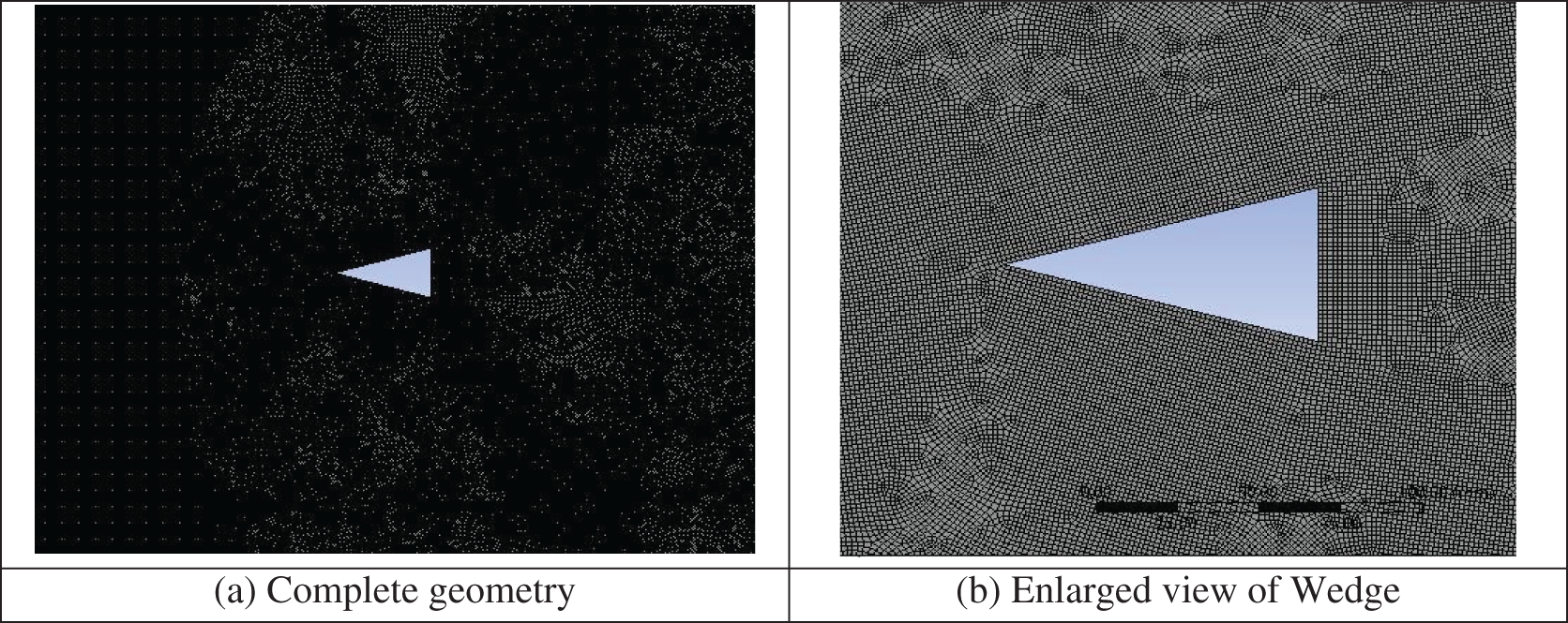
Figure 3: 2D meshed geometry for Mach = 12 and θ = 10° and mesh element size 3 mm
The entire CFD analysis is performed by using all the possible combinations of parameters. Pathan et al. [29] have studied enlarged duct length optimization in the case of suddenly expanded flows. The solution is started by setting a boundary condition and runs for at least 10000 iterations. In many cases, the solution converges after 1000 iterations.
For the analysis, the viscous k-epsilon turbulent model is adopted. The boundary conditions are specified by inlet as velocity inlet and outlet as pressure outlet. According to the Mach number, the velocity is calculated and set at inlet velocity. The pressure at the outlet is set to zero atmosphere. The SIMPLE approach is used during the analysis. The central differences in spatial numerical schemes are adopted for the analysis, and a first-order accuracy is considered. As the flow is supersonic and compressible, the problem density-based solver is considered for the analysis. The equations considered for a fluid flow analysis are continuity equation, momentum equation, and energy equation are written in Eqs. (4)–(6), respectively.
2.4 Validation of Present Work with Literature
The results obtained from CFD analysis have been validated with the results available in the literature and shown in Fig. 4. Crasta et al. [30] have analytically studied and computed pressure on the nose of the 2D Wedge at Mach number = 10. Fig. 4 shows an excellent agreement between the results of pressure variation with the analytical study and the present research work.
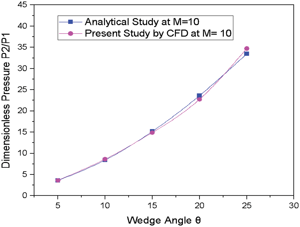
Figure 4: Comparison between the analytical study of Variation of dimensionless pressure and the Variation of dimensionless pressure at M = 10
2.5 Results of Pressure Contours
Fig. 5 shows the pressure contours for various Mach numbers at the angle of incidence 10°. Based on the results, it can be seen that the Mach cone angle reduces when the Mach number increases.
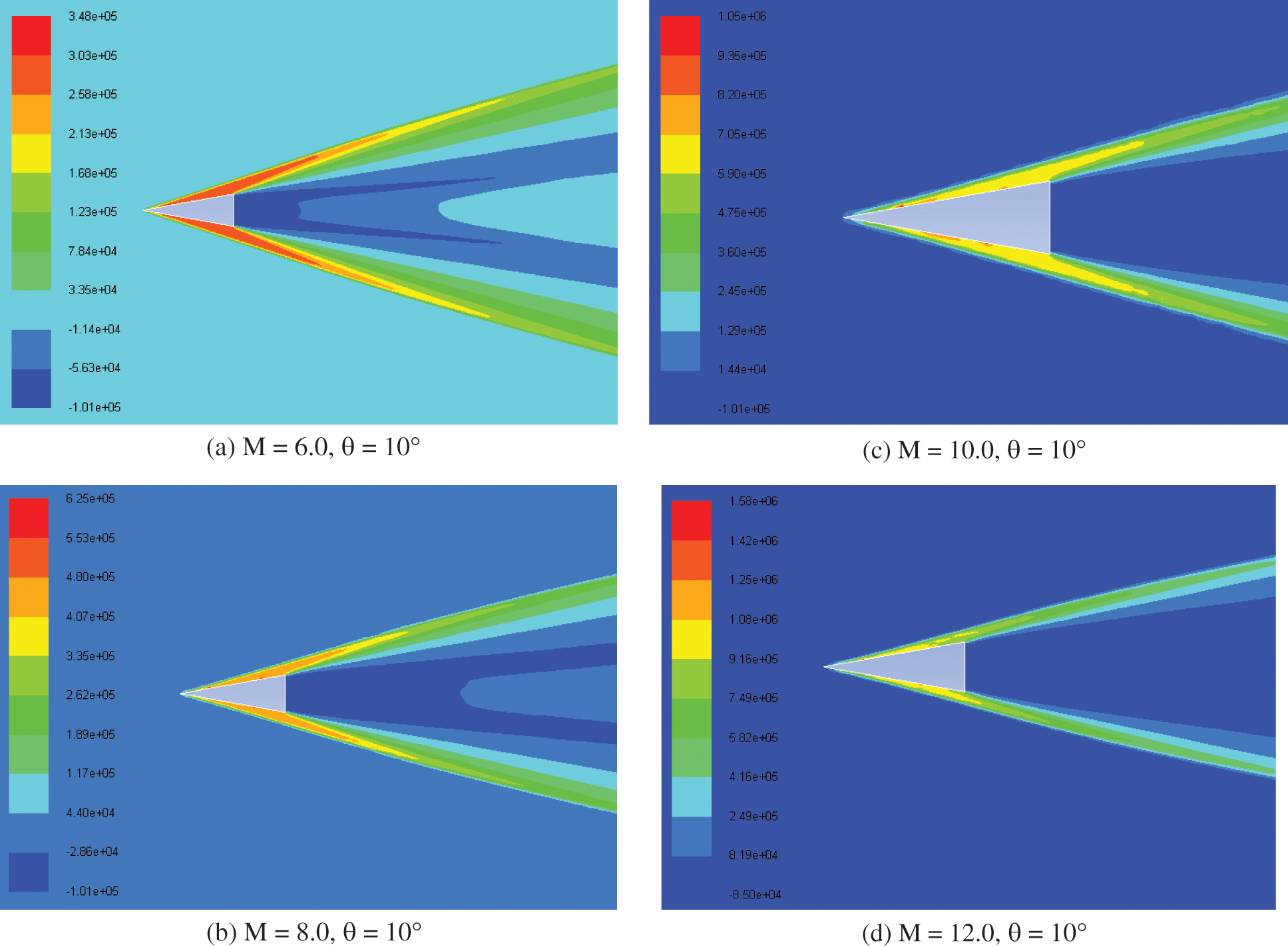
Figure 5: Contours of static pressure for various Mach numbers and angle of incidence θ = 10°
2.6 Results of Mach Number Contours
Fig. 6 shows the contours of Mach numbers at a constant angle of incidence 10° for various inlet Mach numbers from 6.0 to 12. Based on the results, it can be seen that the Mach cone angle reduces when the Mach number increases.
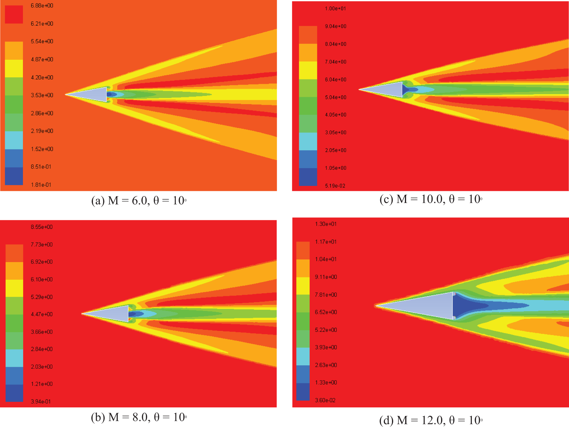
Figure 6: Contours of Mach number at the angle of incidence 10° and various inlet Mach numbers
2.7 CFD Results of Pressure at Various Locations along the Length of the Wedge for a Constant Mach Number
The CFD analysis results for the pressure along the edge of wedge length (x/L) at constant Mach numbers have been extracted from ANSYS Fluent software and plotted in Figs. 7–16. The static pressure values are converted into dimensionless pressure by dividing it by atmospheric pressure.
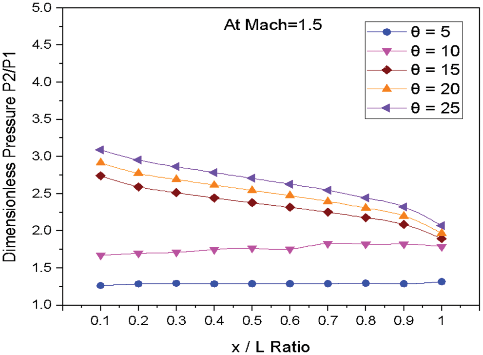
Figure 7: Variation of dimensionless pressure vs. x/L ratio at M = 1.5
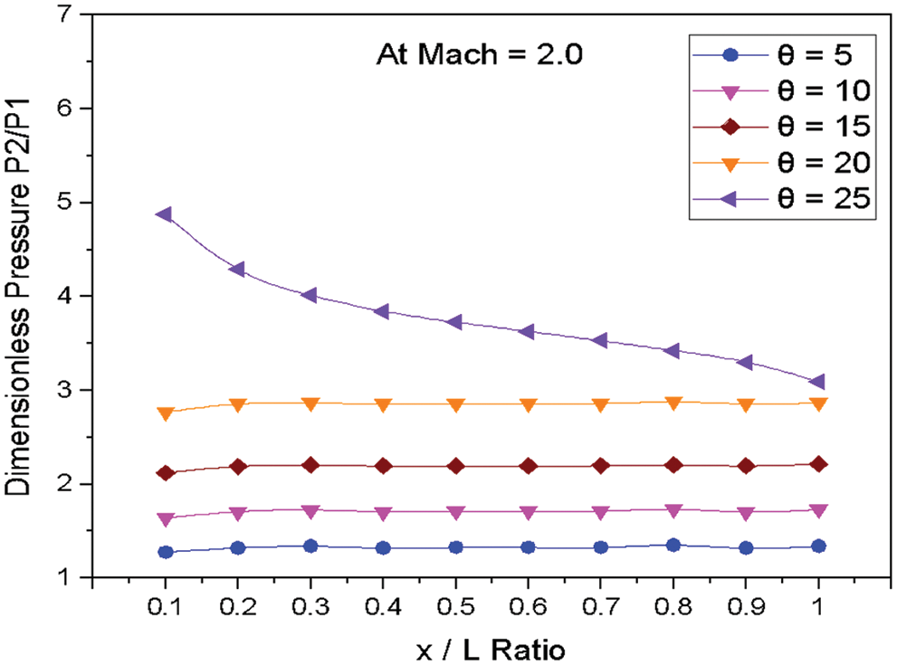
Figure 8: Variation of dimensionless pressure vs. x/L ratio at M = 2.0
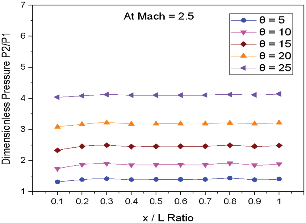
Figure 9: Variation of dimensionless pressure vs. x/L ratio at M = 2.5
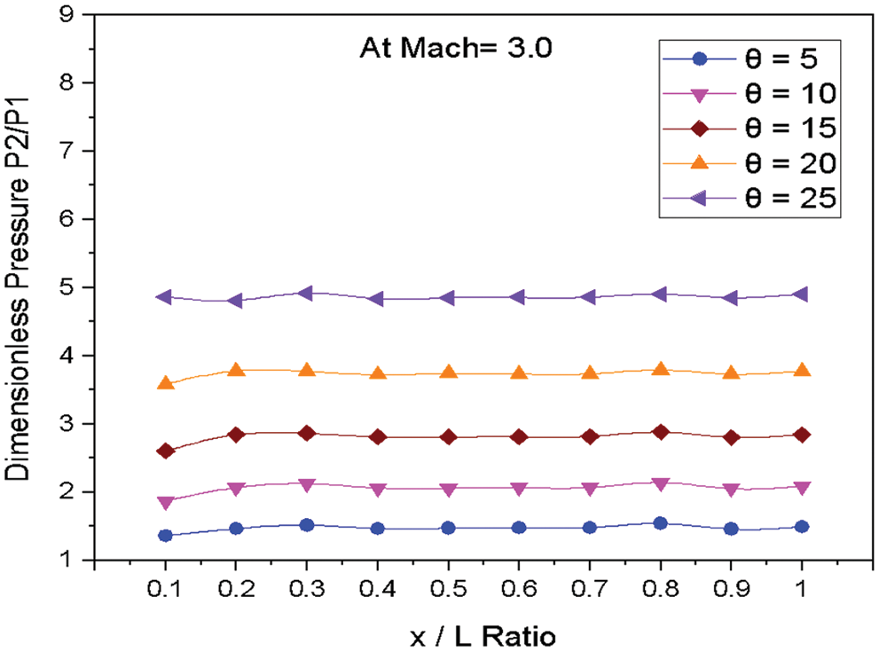
Figure 10: Variation of dimensionless pressure vs. x/L ratio at M = 3.0
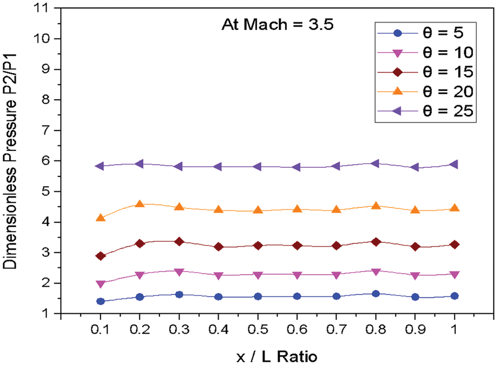
Figure 11: Variation of dimensionless pressure vs. x/L ratio at M = 3.5
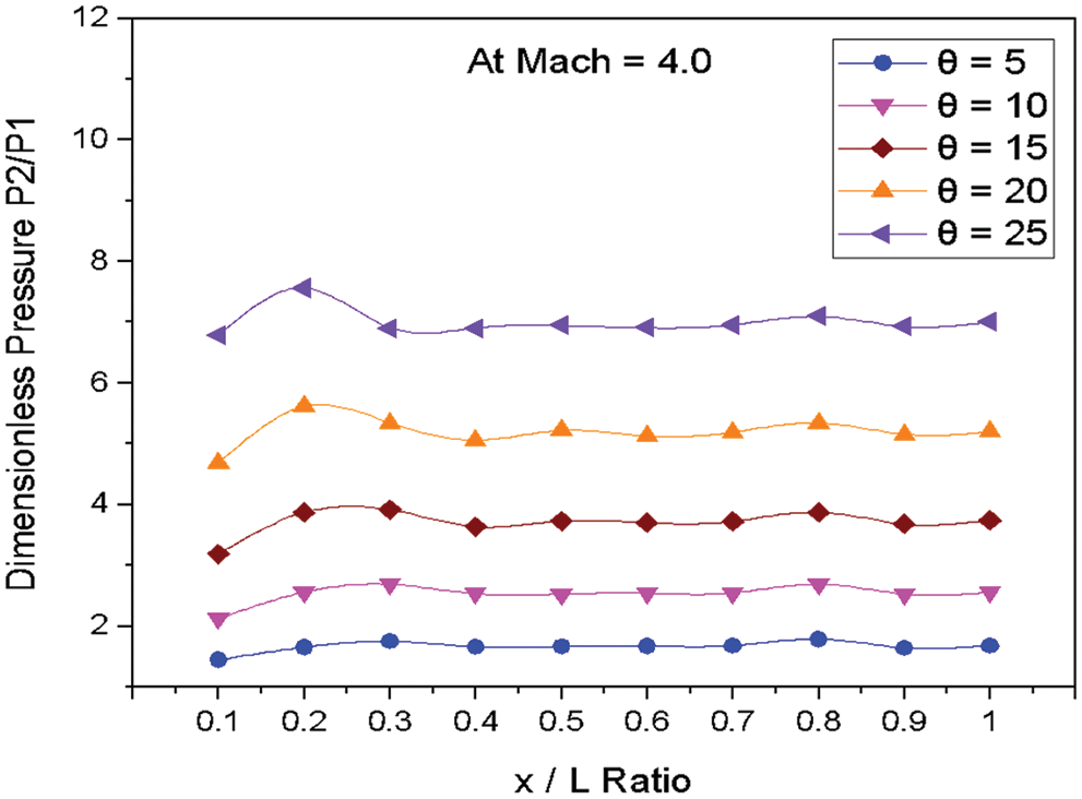
Figure 12: Variation of dimensionless pressure vs. x/L ratio at M = 4
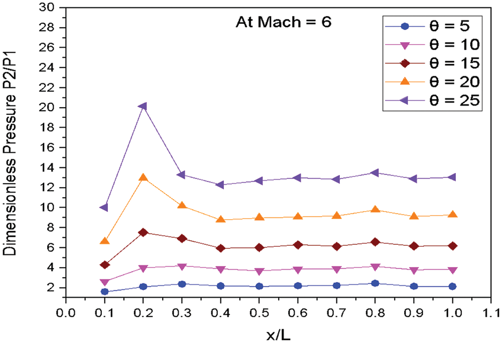
Figure 13: Variation of dimensionless pressure vs. x/L ratio at M = 6
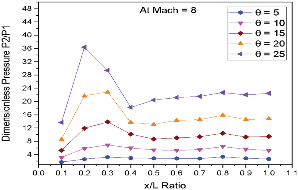
Figure 14: Variation of dimensionless pressure vs. x/L ratio at M = 8.0
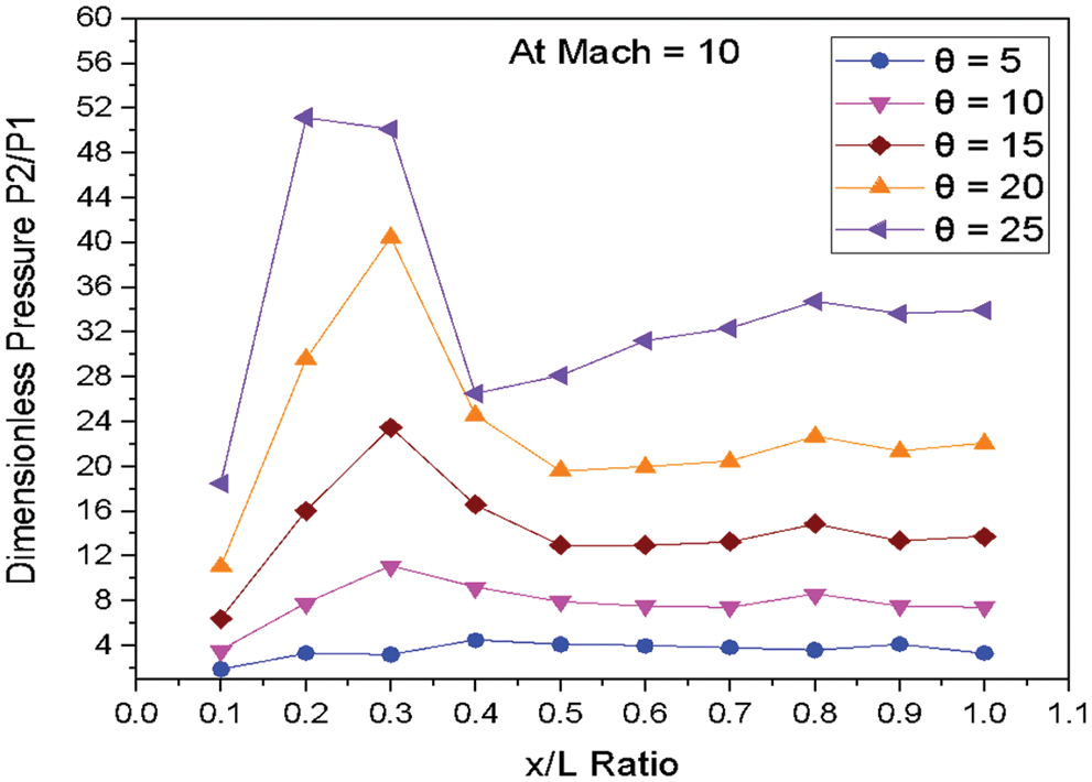
Figure 15: Variation of dimensionless pressure vs. x/L ratio at M = 10
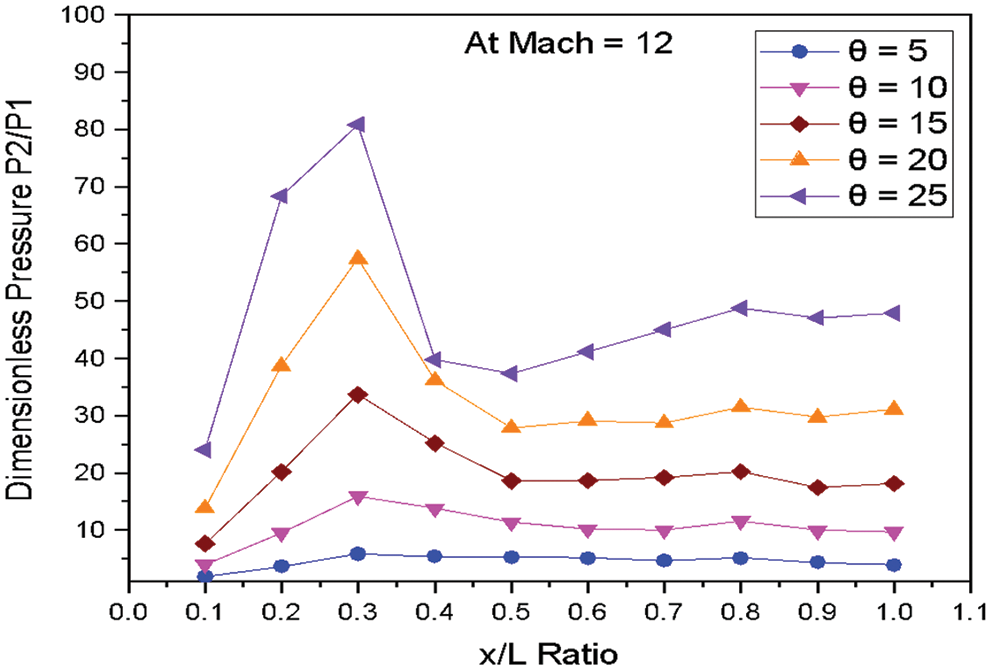
Figure 16: Variation of dimensionless pressure vs. x/L ratio at M = 12.0
Fig. 7 shows the variations of dimensionless static pressure vs. the location along the edge of wedge length (x/L) at constant Mach number M = 1.5 for various angles of incidences. From the results, it is clear that as the angle of incidence increases, the static pressure increases at the nose of the Wedge. Along the edge of the 2D Wedge, the pressure decreases for the wedge angle from 15° to 25°. The change in the pressure is negligible along the wedge length for the wedge angle from 5° to 10°.
Fig. 8 shows the variations of dimensionless static pressure vs. along the edge of wedge length (x/L) at constant Mach number M = 2.0 for various angles of incidences. From the results, it is clear that as the angle of incidence increases, the pressure increases at the nose of the Wedge. Then afterward, there is an insignificant change in pressure along the edge of the wedge length for the angle of 5° to 20°. The sudden change in pressure is observed as the angle of incidence changes from 20° to 25° at the nose of the Wedge. The pressure decreases along the wedge length for the angle of 25°.
Fig. 9 shows the variations of dimensionless static pressure vs. along the edge of wedge length (x/L) at constant Mach number M = 2.5 for various angles of incidences. From the results, it is clear that as the angle of incidence increases, the pressure increases at the nose of the Wedge. The marginal variation in pressure is observed along the edge of the wedge length for the angle of 5° to 25°.
Fig. 10 shows the variations of dimensionless static pressure vs. along the edge of wedge length (x/L) at constant Mach number M = 2.5 for various angles of incidences. From the results, it is clear that as the angle of incidence increases, the pressure increases at the nose of the Wedge. There are marginal variations observed in pressure along the edge of the wedge length for the angle of 5° to 25°.
Fig. 11 shows the variations of dimensionless static pressure vs. along the edge of wedge length (x/L) at constant Mach number M = 3.5 for various angles of incidences. It is seen that the pressure increases at the nose of the Wedge as the angle of incidence increases. The pressure increases at the location x/L = 0.2 for the wedge angle of 15° to 25°.The marginal changes in pressure along the edge of the wedge length for the angle of 5° to 25°.
Fig. 12 shows the variations of dimensionless static pressure vs. along the edge of wedge length (x/L) at constant Mach number M = 4.0 for various angles of incidences. The pressure increases at the nose of the Wedge as the angle of incidence increases. A further increase in pressure is observed at the location x/L = 0.2 for the wedge angle of 5° to 25°. The pressure is decreased from location 0.2 to 0.3 for the wedge angle 5° to 25°. The marginal changes in pressure are observed from the location 0.3 to 1.0 along the edge of the wedge length for the angle of 5° to 25°.
Fig. 13 shows the variations of dimensionless static pressure vs. along the edge of wedge length (x/L) at constant Mach number M = 6.0 for various angles of incidences. The pressure increases at the nose of the Wedge as the angle of incidence increases. The sudden increase in pressure is observed at the location x/L = 0.2 for the wedge angle of 5° to 25°. The pressure is decreased from location 0.2 to 0.3 for the wedge angle 5° to 25°. The marginal changes in pressure from the location 0.3 to 1.0 along the edge of the wedge length for the angle of 5° to 25°.
Fig. 14 shows the variations of dimensionless static pressure vs. along the edge of wedge length (x/L) at constant Mach number M = 8.0 for various angles of incidences. The pressure increases at the nose of the Wedge as the angle of incidence increases. A sudden increase in pressure is observed at the location x/L = 0.1 to 0.3 for the wedge angle 5° to 20°. The pressure decreases at the location from x/L = 0.3 to 0.4 for the wedge angle 5° to 20°. The marginal changes in pressure from the location 0.4 to 1.0 along the edge of the wedge length for the angle of 5° to 25°.
Fig. 15 shows the variations of dimensionless static pressure vs. along the edge of wedge length (x/L) at constant Mach number M = 10.0 for various angles of incidences. The pressure increases at the nose of the Wedge as the angle of incidence increases. The sudden increase in pressure is observed at the location x/L = 0.1 to 0.3 for the wedge angle 5° to 20°. The pressure decreases at the location from x/L = 0.3 to 0.5 for the wedge angle 5° to 20°. The marginal fluctuation in pressure from the location is 0.4 to 1.0 along the edge of the wedge length for the angle of 5° to 25°.
Fig. 16 shows the variations of dimensionless static pressure vs. along the edge of wedge length (x/L) at constant Mach number M = 12.0 for various angles of incidences. The pressure increases at the nose of the Wedge as the angle of incidence increases. The sudden increase in pressure is observed at the location x/L = 0.1 to 0.3 for the wedge angle 5° to 25°. The pressure decreases at the location from x/L = 0.3 to 0.5 for the wedge angle 5° to 25°. The marginal fluctuation in pressure from the location is 0.5 to 1.0 along the edge of the wedge length for the angles from 5° to 25°.
2.8 CFD Results of Pressure at Various Locations along the Length of the Wedge for a Constant Angle of Incidence
The CFD analysis results for the pressure along the edge of wedge length (x/L) at constant Mach numbers have been extracted from ANSYS Fluent software and plotted in Figs. 17–21. The static pressure values are converted into dimensionless pressure by dividing it by atmospheric pressure.
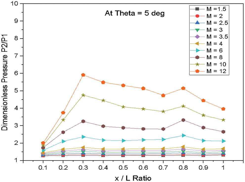
Figure 17: Variation of dimensionless pressure vs. x/L ratio at θ = 5°
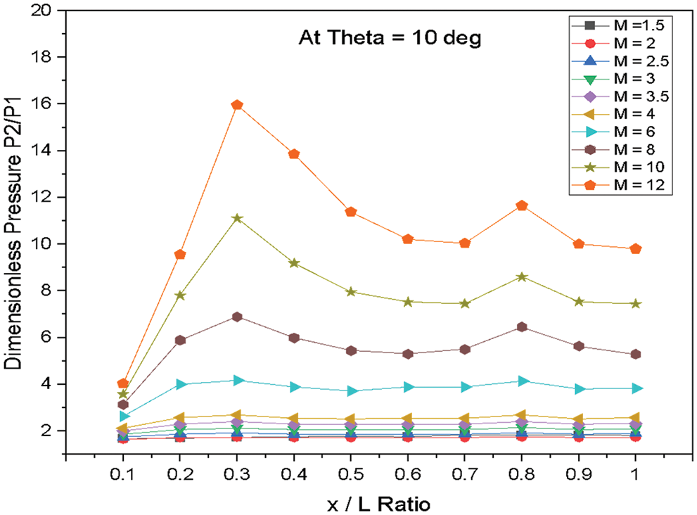
Figure 18: Variation of dimensionless pressure vs. x/L ratio at θ = 10°
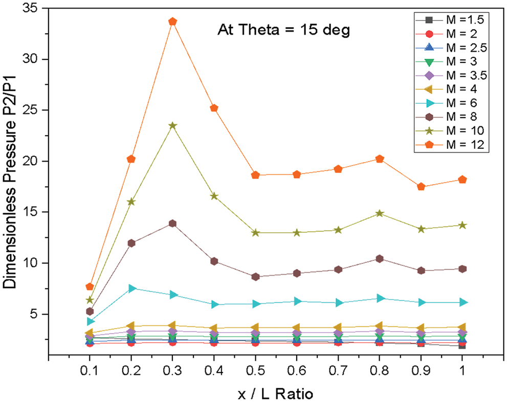
Figure 19: Variation of dimensionless pressure vs. x/L ratio at θ = 15°

Figure 20: Variation of dimensionless pressure vs. x/L ratio at θ = 20°
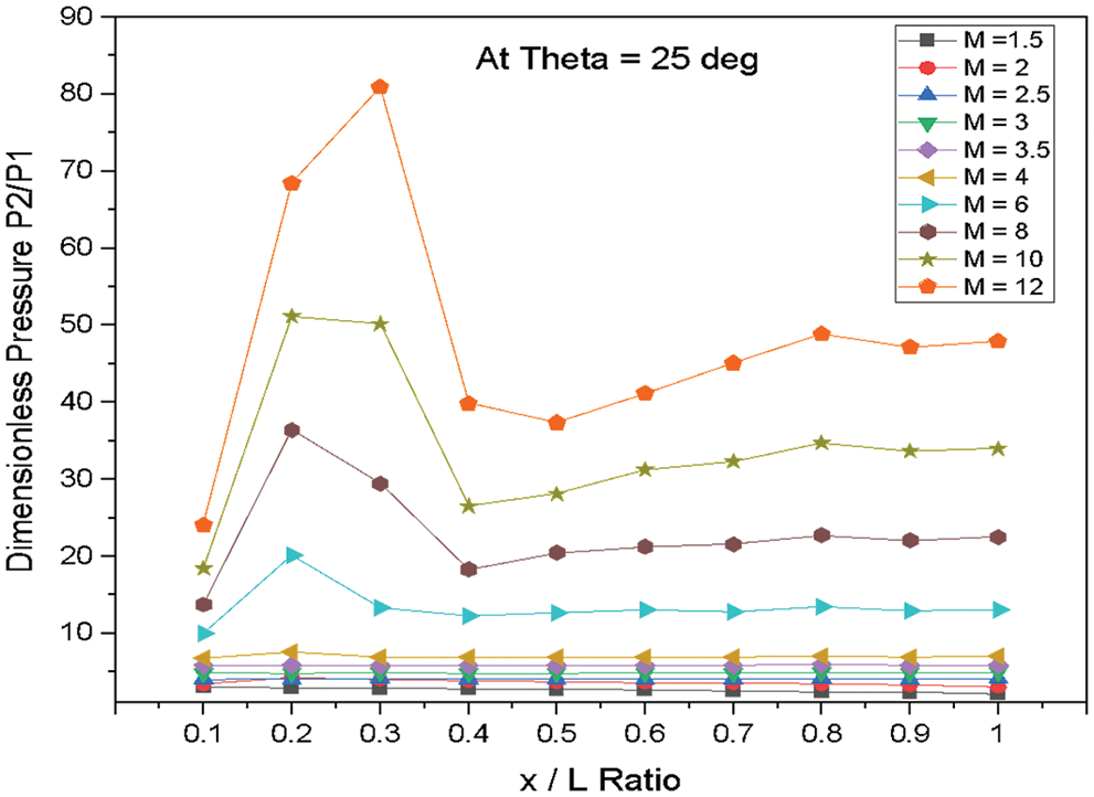
Figure 21: Variation of dimensionless pressure vs. x/L ratio at θ = 25°
Fig. 17 shows the variations of dimensionless static pressure vs. along the edge of wedge length (x/L) at a constant angle of incidence θ = 5° for various Mach numbers. The results show that the pressure increases from the nose of the Wedge to the location x/L = 0.3 for the higher Mach numbers from M = 4 to 12, and then the pressure reduces and fluctuates after the location x/L = 0.3. For the lower Mach number from M = 1.5 to 3.5, there is a marginal change in the pressure along the edge of the wedge length.
Fig. 18 shows the variations of dimensionless static pressure vs. along the edge of wedge length (x/L) at a constant angle of incidence θ = 10° for various Mach numbers. From the results, it is observed that there is a continuous increase in pressure from the nose of the Wedge to the location x/L = 0.3 for the higher Mach numbers from M = 4 to 12. Then the pressure gets reduced and fluctuates after the location x/L = 0.3. For the Mach number from M = 1.5 to 3.5 change in the pressure along the edge of the Wedge, length is observed as marginal change.
Fig. 19 shows the variations of dimensionless static pressure vs. along the edge of wedge length (x/L) at a constant angle of incidence θ = 15° for various Mach numbers. From the results, it is observed that there is a continuous increase in pressure from the nose of the Wedge to the location x/L = 0.3 for the higher Mach numbers from M = 4 to12. Then the pressure reduces and fluctuates after the location at x/L = 0.3.
Fig. 20 shows the variations of dimensionless static pressure vs. along the edge of wedge length (x/L) at a constant angle of incidence θ = 20° for various Mach numbers. From the results, it is observed that there is a continuous increase in pressure from the nose of the Wedge to the location x/L = 0.3 mm for the higher Mach numbers from M = 4 to 12. Then the pressure decreases and fluctuates after the location x/L = 0.3. The change in the surface pressure along the edge of the wedge length is observed as a marginal change for lower Mach numbers.
Fig. 21 shows the variations of dimensionless static pressure vs. along the edge of wedge length (x/L) at a constant angle of incidence θ = 25° for various Mach numbers. From the results, it is clear that there is a continuous increase in pressure from the nose of the Wedge to the location at x/L = 0.3 for the higher Mach numbers from M = 4 to 12, and then the pressure gets reduced and fluctuates after the place at x/L = 0.3. The only marginal change was observed in the pressure for the Mach number from M = 1.5 to 3.5.
The regression formula is developed using the Minitab software, and the results for dimensionless static pressure are evaluated for the parameters Mach number (M), angle of incidence (T), and x/L ratio (L). The regression model for dimensionless static pressure is given by Eq. (7).
Fig. 22 shows the variations of dimensionless static pressure vs. along the edge of the wedge length (x/L) for various Mach numbers and angles of incidence. The results clearly show excellent agreement, and the CFD results and results were obtained using regression model pressure. The absolute static pressure is divided by atmospheric pressure to non-dimensionalized pressure; as the Mach number increases, the dimensionless pressure increases at the nose of the Wedge for all Mach numbers and all angles of incidence. The CFD results reveal that for the higher Mach numbers and the higher angle of incidence, i.e., for M = 4 to M = 12. From θ = 15° to θ = 25°, the pressure increases till up to the location x/L = 0.3, then it decreases and fluctuates with marginal variation in the pressure over the location from x/L = 0.3.
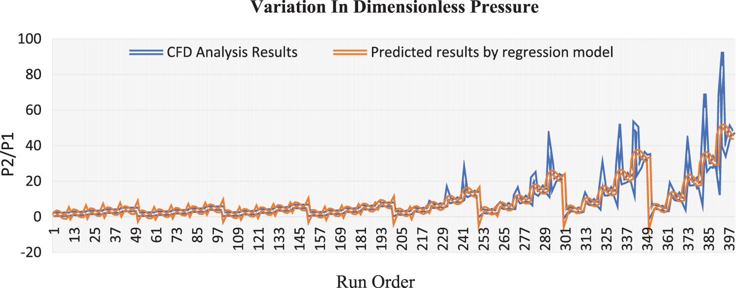
Figure 22: Variation of dimensionless pressure vs. x/L ratio for different flow parameters combinations
The above research work exhibits its extensive range of applications in the angle of incidence, Mach number, and edge of the Wedge. Based on the above results, it can be concluded that the dimensionless static pressure increases with the increase in Mach numbers and incidence angle at the Wedge’s nose. For the lower Mach numbers from M = 1.5 to 3.5, there is marginal variation in pressure in all locations of the edge of the wedge length. As the Mach number increases from M = 4.0 to 12, there is a continuous increase in pressure up to location x/L = 0.3. Then the pressure will decrease from the location x/L = 0.3 with fluctuation in the pressure value. It is also observed that for all the angles of incidence, the change in pressure value is very insignificant for the Mach number M = 1.5 to 3.5 in all the locations of the edge of the wedge length. As the Mach number increases from M = 4.0 to 12, there is a sudden increase in pressure value up to the location x/L = 0.3. After this location, there is a downfall in the pressure value with marginal fluctuation for all angles of incidence. The present study gives good results with incredible computational ease. These results are beneficial to optimizing the design stage of an aerospace vehicle. So, to optimize the design of aerospace vehicles, these results can be used as the cost involved in wind tunnel tests is very high.
Funding Statement: The authors received no specific funding for this study.
Conflicts of Interest: The authors declare they have no conflicts of interest to report regarding the present study.
References
1. Tsien, H. (1946). Similarity laws of hypersonic flows. Journal of Mathematics and Physics, 25(1), 247–251. DOI 10.1002/sapm1946251247. [Google Scholar] [CrossRef]
2. Hayes, W. D. (1947). On hypersonic similitude. Quarterly of Applied Mathematics, 5(1), 105–106. DOI 10.1090/qam/20904. [Google Scholar] [CrossRef]
3. Zartarian, G., Hsu, P. T., Ashley, H. (1961). Dynamic air loads and aeroelastic problems at entry mach numbers. Journal of the Aerospace Science, 28(3), 209–222. DOI 10.2514/8.8927. [Google Scholar] [CrossRef]
4. Carrier, G. F. (1949). The oscillating wedge in the supersonic stream. Journal of Aeronautical Sciences, 16(3), 150–152. DOI 10.2514/8.11755. [Google Scholar] [CrossRef]
5. Hui, W. H. (1971). Supersonic and hypersonic flow with attached shock waves over delta wings. Proceedings of The Royal Society A: Mathematical, Physical and Engineering Sciences, 325(1561), 251–268. [Google Scholar]
6. Hui, W. H., Hemdan, H. T. (1976). Unsteady hypersonic flow over delta wings with detached shock waves. American Institute of Aeronautics and Astronautics Journal, 14(4), 505–511. DOI 10.2514/3.7120. [Google Scholar] [CrossRef]
7. Lui, D. D., Hui, W. H. (1977). Oscillating delta wings with attached shock waves. American Institute of Aeronautics and Astronautics Journal, 15(6), 804–812. DOI 10.2514/3.7371. [Google Scholar] [CrossRef]
8. Lighthill, M. J. (1953). Oscillating aerofoil at high mach numbers. Journal of the Aeronautical Sciences, 20(6), 402–406. DOI 10.2514/8.2657. [Google Scholar] [CrossRef]
9. Ghosh, K., Mistry, B. K. (1980). Large incidence hypersonic similitude and oscillating non-planar wedges. American Institute of Aeronautics and Astronautics Journal, 18(8), 1004–1006. DOI 10.2514/3.7702. [Google Scholar] [CrossRef]
10. Miles, J. W. (1960). Unsteady flow at hypersonic speeds, hypersonic flow. London, UK: Butterworths Scientific Publications. [Google Scholar]
11. Ghosh, K. (1984). Hypersonic large deflection similitude for oscillating delta wings. The Aeronautical Journal, 88(878), 357–361. [Google Scholar]
12. Crasta, A., Pavitra, S., Khan, S. A. (2016). Estimation of surface pressure distribution on a delta wing with curved leading edges in hypersonic/supersonic flow. International Journal of Energy, Environment, and Economics, 2(1), 1–7. [Google Scholar]
13. Musavir, B., Khan, S. A., Azam, Q., Janvekar, A. A. (2017). Computational and analytical investigation of aerodynamic derivatives of similitude delta wing model at hypersonic speeds. International Journal of Technology, 3, 366–375. [Google Scholar]
14. Khan, S. A., Aabid, A., Saleel, C. A. (2019). CFD simulation with analytical and theoretical validation of different flow parameters for the wedge at supersonic mach number. International Journal of Mechanical and Mechatronics Engineering, 19(1), 170–177. [Google Scholar]
15. Kalimuthu, R., Mehta, R. C., Rathakrishnan, E. (2019). Measured aerodynamic coefficients without and with the blunt spiked body at Mach 6. Advances in Aircraft Spacecraft Science, 6(3), 225–238. [Google Scholar]
16. Zuhair, M. A. B., Mohammed, A. (2019). Trailing edge geometry effect on the aerodynamics of low-speed BWB aerial vehicles. Advances in Aircraft Spacecraft Science, 6(4), 283–296. [Google Scholar]
17. Meng, Y., Yan, L., Huang, W., Chen, J., Jie, L. (2021). Coupled investigation on drag reduction and thermal protection mechanism of a double-cone missile by the combined spike and multi-jet. Aerospace Science and Technology, 115(1). DOI 10.1016/j.ast.2021.106840. [Google Scholar] [CrossRef]
18. Shaikh, J. S., Kumar, K., Pathan, K. N., Khan, S. A. (2022). Analytical and computational analysis of pressure at the nose of a 2D wedge in high-speed flow. Advances in Aircraft Spacecraft Science, 9(2), 119–130. [Google Scholar]
19. Pathan, K. A., Khan, S. A., Shaikh, A. N., Pathan, A. A., Khan, S. A. (2021). An investigation of the boat-tail helmet to reduce drag. Advances in Aircraft Spacecraft Science, 8(1), 239–250. [Google Scholar]
20. Azami, M. H., Faheem, M., Aabid, A., Mokashi, I., Khan, S. A. (2019). Experimental research of wall pressure distribution and effect of micro jet at Mach 1.5. International Journal of Recent Technology and Engineering, 8(3), 1000–1003. [Google Scholar]
21. Pathan, K. A., Dabeer, P. S., Khan, S. A. (2019). Investigation of base pressure variations in internal and external suddenly expanded flows using CFD analysis. CFD Letters, 11(4), 32–40. [Google Scholar]
22. Khan, S. A., Rathakrishnan, E. (2006). Active control of base pressure in supersonic regime. Journal of the Institution of Engineers (IndiaAerospace Engineering Journal, 87, 3–11. [Google Scholar]
23. Pathan, K. A., Dabeer, P. S., Khan, S. A. (2020). An investigation of effect of control jets location and blowing pressure ratio to control base pressure in suddenly expanded flows. Journal of Thermal Engineering, 6(2), 15–23. DOI 10.18186/thermal.726106. [Google Scholar] [CrossRef]
24. Pathan, K. A., Ashfaq, S., Dabeer, P. S., Khan, S. A. (2019). Analysis of parameters affecting thrust and base pressure in suddenly expanded flow from nozzle. Journal of Advanced Research in Fluid Mechanics and Thermal Science, 64(1), 1–18. [Google Scholar]
25. Pathan, K. A., Dabeer, P. S., Khan, S. A. (2019). Influence of expansion level on base pressure and reattachment length. CFD Letters, 11(5), 22–36. [Google Scholar]
26. Pathan, K. A., Dabeer, P. S., Khan, S. A. (2019). Effect of nozzle pressure ratio and control jets location to control base pressure in suddenly expanded flows. Journal of Applied Fluid Mechanics, 12(4), 1127–1135. DOI 10.29252/jafm.12.04.29495. [Google Scholar] [CrossRef]
27. Khan, A., Mazlan, N. M., Ismail, M. A. (2019). Analysis of flow through a convergent nozzle at sonic mach number for area ratio 4. Journal of Advanced Research in Fluid Mechanics and Thermal Sciences, 62(1), 66–79. [Google Scholar]
28. Rathakrishnan, E. (2012). Gas dynamics. New Delhi: PHI Learning Private Limited. [Google Scholar]
29. Pathan, K. A., Dabeer, P., Khan, S. A. (2020). Enlarge duct length optimization for suddenly expanded flows. Advances in Aircraft Spacecraft Science, 7(3), 203–214. [Google Scholar]
30. Crasta, A., Pavitra, S., Khan, S. A. (2016). Estimation of surface pressure distribution on a delta wing with curved leading edges in hypersonic/supersonic flow. International Journal of Energy, Environment, and Economics, 24(1), 67–73. [Google Scholar]
Cite This Article
 Copyright © 2023 The Author(s). Published by Tech Science Press.
This work is licensed under a Creative Commons Attribution 4.0 International License , which permits unrestricted use, distribution, and reproduction in any medium, provided the original work is properly cited.
 Downloads
 Citation Tools