
 Submit a Paper
 Propose a Special lssue
 Open Access
ARTICLE

The Turbulent Schmidt Number for Transient Contaminant Dispersion in a Large Ventilated Room Using a Realizable k-ε Model
School of Environment and Architecture, University of Shanghai for Science and Technology, Shanghai, 200093, China
* Corresponding Author: Qianru Zhang. Email:
Fluid Dynamics & Materials Processing 2024, 20(4), 829-846. https://doi.org/10.32604/fdmp.2023.026917
Received 02 October 2022; Accepted 20 October 2023; Issue published 28 March 2024
 View Full Text
 Download PDF
Abstract
Buildings with large open spaces in which chemicals are handled are often exposed to the risk of explosions. Computational fluid dynamics is a useful and convenient way to investigate contaminant dispersion in such large spaces. The turbulent Schmidt number (Sct) concept has typically been used in this regard, and most studies have adopted a default value. We studied the concentration distribution for sulfur hexafluoride (SF6) assuming different emission rates and considering the effect of Sct. Then we examined the same problem for a light gas by assuming hydrogen gas (H2) as the contaminant. When SF6 was considered as the contaminant gas, a variation in the emission rate completely changed the concentration distribution. When the emission rate was low, the gravitational effect did not take place. For both low and high emission rates, an increase in Sct accelerated the transport rate of SF6. In contrast, for H2 as the contaminant gas, a larger Sct could induce a decrease in the H2 transport rate.Keywords
Nomenclature
| Sct | Turbulent Schmidt number |
| | Density of the fluid |
| | Scalar |
| t | Time |
| | Velocity vector |
| | Diffusion coefficient |
| | Source term |
| | Turbulent viscosity |
| | Turbulent diffusivity |
| ui | Velocity in the ith direction |
| | Dynamic viscosity |
| | Thermal conductivity |
| d | Diffusion coefficient for the species in the mixture |
| | Specific heat at constant pressure |
| T | Temperature |
| | Mass fraction of the ith species |
| P | Pressure |
| c | Concentration |
| Q | Thermal energy |
| | Source emission rate |
| g | Gravitational acceleration |
| k | Turbulence kinetic energy |
| | Rate of dissipation for turbulence kinetic energy |
| Gk | Generation of turbulence kinetic energy due to the mean velocity gradients |
| Gb | Generation of turbulence kinetic energy due to buoyancy |
| YM | Contribution of the fluctuating dilatation in compressible turbulence to the overall dissipation rate |
| | Constant |
| | Constant |
| | Constant |
| σk | Turbulent Prandtl number for k |
| | Turbulent Prandtl number for ε |
| Sk | User-defined source term |
| | user-defined source term |
| Cμ | Constant |
| C | The concentration of SF6 |
| C0 | Contaminant concentration when the room is fully mixed |
| q | Contaminant emission rate |
| Qv | Room ventilation rate |
Environmental risk assessment is often associated with open areas due to the accidents that occur in chemical processing installations, which are built in such areas. Many researchers have focused on dense gas dispersion in the atmospheric environment and have proposed theoretical models to solve the dense gas dispersion problem [1–4]. Nevertheless, there are still exist accidental release of a sustained, small, undetected leak of a dense toxic gas (chlorine) in an industrial indoor environment in which the risk posed by the indoor handling of chemicals must be assessed [5].
With the development of computational fluid dynamics (CFD), an increasing number of studies have used simulation [6]. The turbulent Schmidt number (Sct) is a necessary parameter in the simulation of gas dispersion in ventilated rooms. Sct was proposed to calculate turbulent diffusivity:
After comparing simulations with experimental data, Spalding [7] recommended an Sct value of 0.7. As Bady et al. [8] pointed out, however, Sct is not constant and varies from one location to another within the same calculation domain. Tahmooresi et al. [9] simulated seven scenarios with different values of Sct, and the results showed that changing the turbulent Schmidt number has significant consequences for mixing and geometrical parameters. Balestrin et al. [10] presented an alternative to better predict turbulent catalytic systems with surface reaction limited by mass transfer selecting an optimal turbulent Schmidt number (Sct varying from 0.2 to 1.1). Other researchers have conducted studies related to different Sct value [11–13].
When studying Sct, knowledge of the turbulent diffusivity is required. Based on the analogy between the exchange of mass and momentum, the turbulent viscosity (momentum) is usually used instead of the turbulent diffusivity of mass [14]. The specific Sct has a significant effect on the prediction results [15]. Most researchers have assumed Sct to be a constant.
Within the study of the atmosphere, it is recommended that Sct be determined by considering the dominant flow structure in each case, and Tominaga et al. [15] classified the literature into categories accordingly. In the jet-in-crossflow field, He et al. [16] gave the Sct expression along the jet and proved that Sct is a variable instead of a constant in a simulation based on Kamotani et al. [17] velocity and temperature trajectories. They also studied species spreading in jet-in-crossflow with different momentum ratios between the jet and the crossflow. An Sct of 0.2 was recommended for optimal agreement with the experimental data. However, as remarked in Tominaga et al. [15], the predicted turbulence intensity around the jet given by this computation is underestimated in comparison with the experiment, which can be compensated for in this case by the large Sct. If this assumption is correct, the optimum value of 0.2 recommended in that study is indeed very low. In the dispersion in boundary layers, the optimum Sct is widely distributed in the range of 0.2–1.3 in the atmospheric dispersion field [15]. Koeltzsch [14] conducted wind tunnel experiments of the flow above a plate and demonstrated that, within the boundary layer, Sct has a strong dependence on height. By fitting the experimental data, a power series was proposed to calculate the Sct in the boundary layer. In regard to plume dispersion in the boundary layer, a smaller Sct value is supposed to increase the turbulent diffusion near the ground. For concentrations around plumes in open country and around a single building, a smaller value of Sct such as 0.3 tends to provide more accurate predictions of concentration distribution. A smaller value of Sct can compensate for the underestimation of the turbulent diffusion for momentum. In Tominaga et al. [15], other types of flows were also investigated. For turbidity currents, for example, the authors recommend a higher value of Sct. As Gromke et al. [18] state, the Sct in a given flow field is spatially variable. It is a fitting parameter that depends on the mean and turbulent characteristics of a flow field, on the position(s) and type(s) of the pollutant source(s), and on the abundance and the heterogeneity of the distribution of the pollutant species in space. They used four normalized merits to judge the Sct for pollutant dispersion simulations in an urban neighborhood, with an Sct value of 0.5.
Few studies, however, have investigated Sct in the pollutant dispersion in indoor simulations. Moreover, most researchers use a constant Sct, as summarized in Table 1.
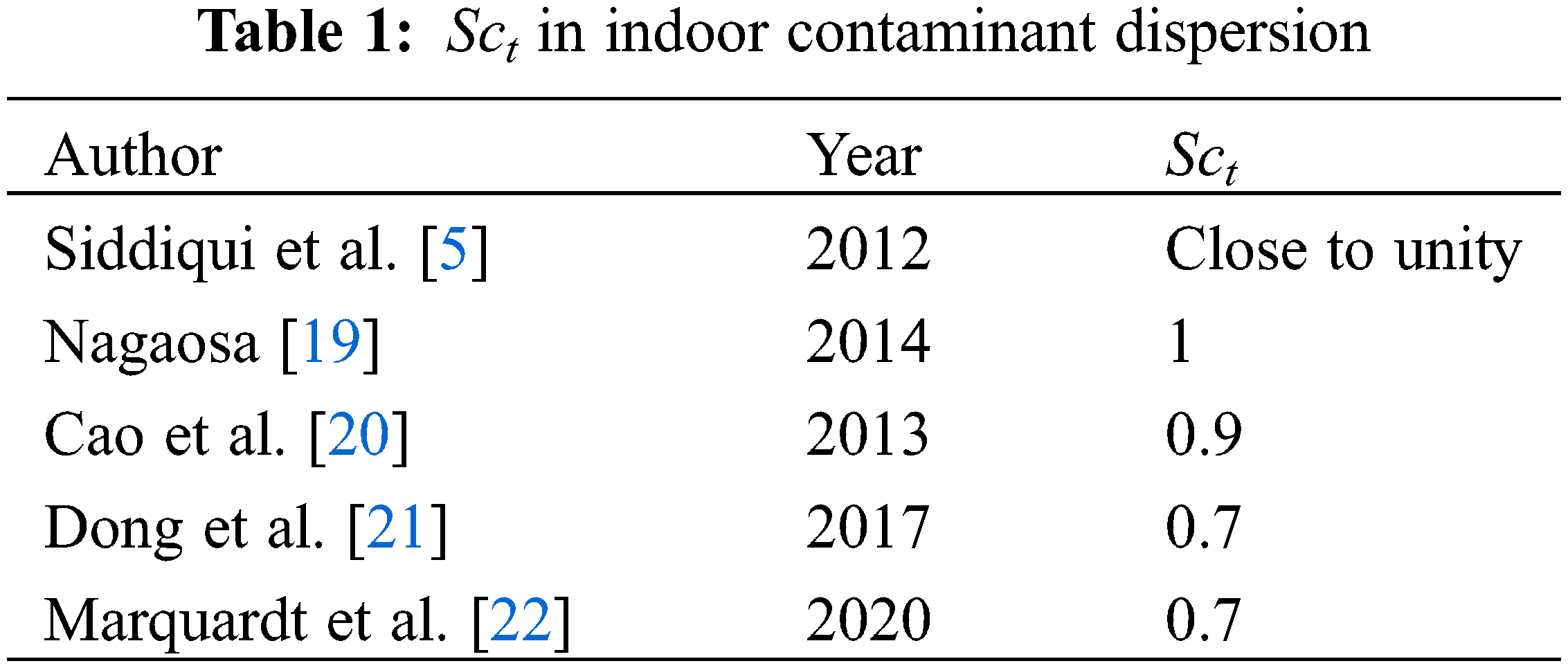
Table 1 shows that, when researchers modified the default value of Sct (0.7), they usually changed it to 1 or 0.9. Shi et al. [23] introduced a new dynamic Sct model for the simulation of stratified flows. Li et al. [24] proposed another Schmidt number model for contaminant dispersion in an indoor environment. These two studies share a similar procedure, namely to calibrate the models with two experimental conditions using two levels of the dimensionless numbers to obtain the constant values. The objects are different, however. In Shi et al. [23], the object is the stratified flow, and the dimensionless number is the Richardson number. In Li et al. [24], the researchers assumed that indoor contaminant dispersion is related to the vortex structures and thus the dimensionless number is the Okubo–Weiss Q value.
In summary, under indoor pollutant dispersion simulation, Sct is a necessary parameter for calculating turbulent diffusivity, and many researchers set it as a default value in the simulation, but this is not very rigorous, each pollutant has different effects on Sct, and modifying Sct arbitrarily may have a large impact on the simulation results. In this paper, SF6 with high density and H2 with low density are selected as research objects to explore their effects on Sct, and the conclusions can play a certain guiding role for the subsequent researchers to conduct numerical simulations.
A 5 × 6 × 6 (length, width, height in meters) chamber was constructed with a steel frame and glass, as shown in Fig. 1. Good airtightness was assumed.
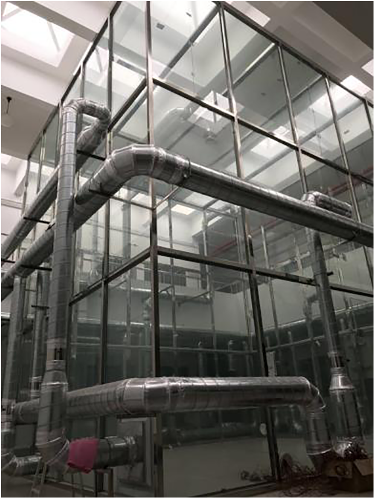
Figure 1: Overview of the chamber
Note: Figure source: Zhang et al. [25].
Two ventilation openings were chosen to perform the air distribution, as shown in Figs. 2a and 2b, which are located in the middle and bottom of the wall. Both grilles have a diameter of 165mm, and the effective area ratio is 53.3%. The grilles locations are illustrated in Fig. 2b.
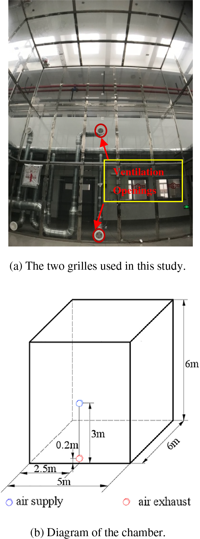
Figure 2: Diagram of the lab and positions of the ventilation openings
Note: Figure source: Zhang et al. [25].
The photoacoustic gas monitor (0–500 ppm ±3%, INNOVA 1412i) was connected to the pipes to record the test point concentration, and the contaminant gas was released at a set point. Anemometers (0.05–30 m/s ± 0.05 m/s) were used to record the velocity at several places. The samplers are depicted in Fig. 3.
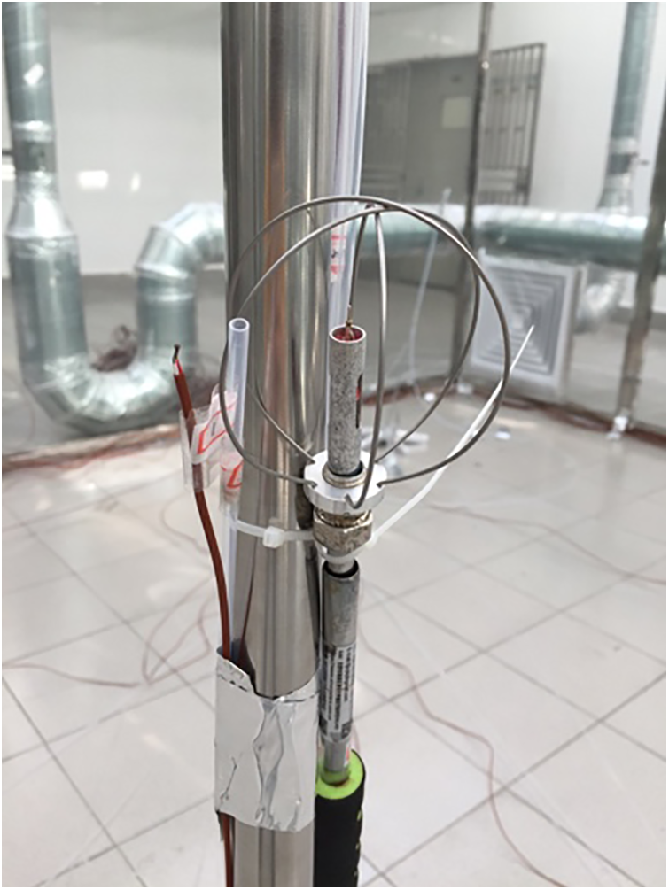
Figure 3: Contaminant sampler and anemometer head
Note: Figure source: Zhang et al. [25].
The contaminant source position and the measure point positions are presented in Fig. 4. In each of the experiments, the contaminant source is located at A or B (3 or 1 m from the floor).
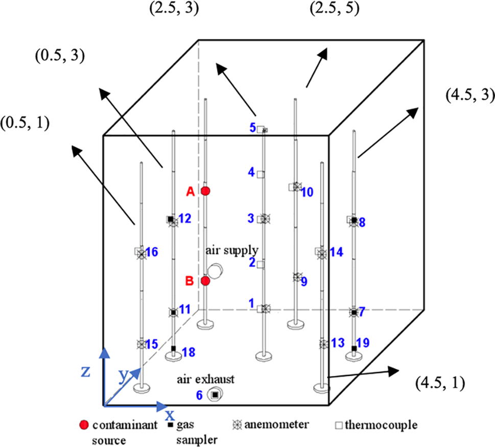
Figure 4: Measurement points in the experimental chamber
Note: Figure source: Zhang et al. [25].
The contaminant point source was modeled by a table tennis ball on which was uniformly distributed 288 holes of 0.5 mm diameter, as shown in Fig. 5. More details of the experiments can be found in Zhang et al. [25].
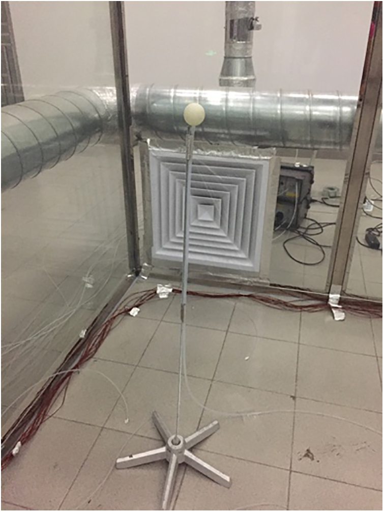
Figure 5: The contaminant point source
Note: Figure source: Zhang et al. [25].
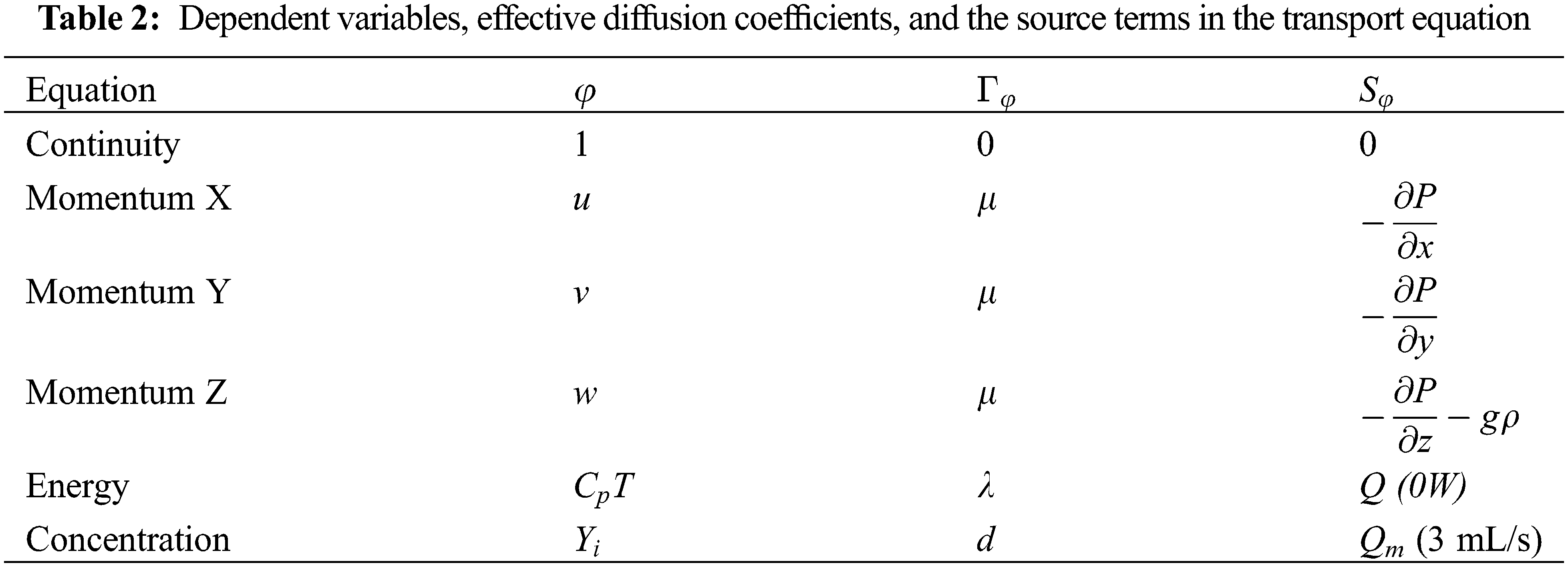
Several ventilation conditions were analyzed in Zhang et al. [25]. One of the experiments was chosen as the benchmark for this study, as shown in Table 2. In that experiment, the air was supplied from the middle opening and exhausted from the bottom. The air change rate was 3 h−1, and the contaminant source rate was 3 mL/s, which was located at A (3 m above the floor).
The ANSYS Fluent was used for the transient Reynolds-averaged Navier–Stokes (RANS) computations based on a control volume approach for solving flow and mass fraction equations. The Green–Gauss cell-based scheme was used for gradient discretization. The advection terms were discretized using a second-order upwind scheme. The semi-implicit method for the pressure-linked equation (SIMPLE) algorithm was used for the pressure-velocity coupling. The spatial discretization for the gradient was least squares cell-based by default and for pressure altered to standard. The rest of the spatial discretization was all set to second-order upwind.
The spatial distribution of airflow, temperature, and species in the zone is governed by the conservation laws of mass, momentum, and energy. The governing advection–diffusion equations of the fluid are all in the following form [26,27]:
The dependent variables, effective diffusion coefficients, and the source terms for each equation are presented in Table 2.
In ANSYS Fluent, the local mass fraction of the species, Yi, was calculated by solving a convection–diffusion equation for the species with the parameter in the last row of Table 2.
3.2 Domains and Computational Grid
The indoor airflow was generated by the jet at the inlet and the flow at the source. Because the chamber was large compared with the inlet opening, a large pressure gradient occurred. Near the jet, a large pressure gradient existed because of the high inlet velocity and the small environment velocity. Near the source, the source velocity was small compared with the environment velocity; the concentration gradient was substantial at the outlet. Thus, close to the air inlet and the contaminant source, fine grids were employed.
The general idea was to create three zones, denominated as JET_ZONE, SOURCE_ZONE, and BODY_ZONE, as shown in Fig. 6.
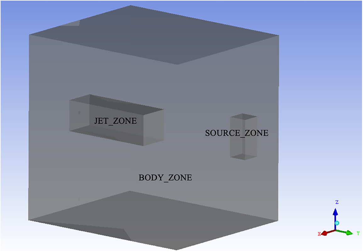
Figure 6: Subdivisions of the large space
The JET_ZONE was the area around the jet, which had a high velocity at the outlet and high gradient of velocity along the jet centerline and the radius of the jet cross-section. The SOURCE_ZONE is the area around the source. There were fine and high-quality mesh (all hexahedral) in this zone.
In the rest of the space, the velocity gradient and the contaminant gradient were both low, and the tetrahedral mesh was sufficient for this zone. The grids division can be seen in Fig. 7. Figs. 7a and 7b show the distribution of grids in parts JET_ZONE and SOURCE_ZONE, respectively.
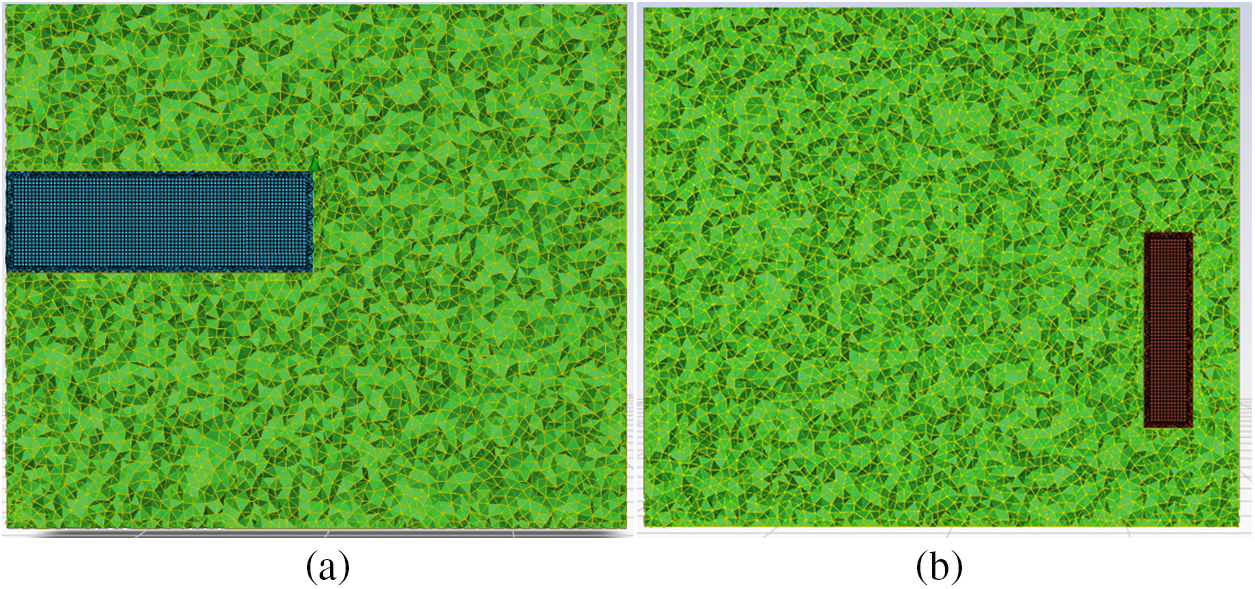
Figure 7: Grid division diagram
Four sets of grids were used to simulate the velocity field with the standard k-ε model and standard wall function. The grid numbers were 1.0 million, 1.5 million, 2.0million and 2.5 million. Fig. 8 shows the comparison of the velocity field for different grid numbers under test line of x = 2.5 m, y = 3 m and x = 2.5 m, y = 5 m.
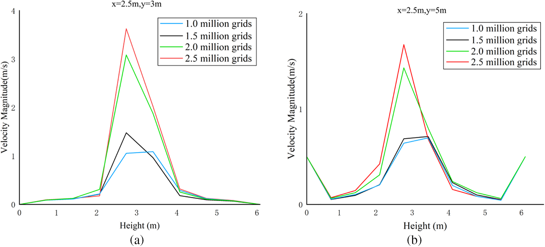
Figure 8: Comparison of velocity field for different grid numbers
As can be seen from Fig. 8, the overall trend of the velocity field of the four grid numbers are the same, indicating that the number of grids selected in this paper can meet the computational requirements. For 1.0 million grids and 1.5 million grids, due to the larger size of the grids, there are some differences in the results computed with the remaining two grids. The 2.0 million grid proved to be fine enough for the velocity field simulation. It was therefore used in the following simulations.
The turbulent Schmidt number is a necessary parameter used to calculate the turbulent diffusivity when simulation indoor gas dispersion; it is a fitting parameter that depends on the mean and turbulent characteristics of the flow field, the position and type of pollutant source, and so on. In RANS models, the variables in the instantaneous Navier–Stokes equations are decomposed into the mean and fluctuating components. For the velocity components,
For pressure and other scalar quantities,
Substituting expressions of this form for the flow variables into the instantaneous continuity and momentum equations and taking time (or ensemble) average (and dropping the overbar on the mean velocity,
The two equations above are called RANS equations. The Reynolds stresses,
A common method employs the Boussinesq hypothesis to relate the Reynolds stresses to the mean velocity gradients:
To model the turbulent viscosity,
and
The turbulent viscosity can be represented by k and ε:
Gb is generation of turbulence kinetic energy due to buoyancy, the formula is
The differences among the various k-ε models concern the values for
We adopted a standard wall function and ensured that most of the wall y star values lay in the region of 15–300.
In the validation case, the air change rate for the space was 3 h−1. For the contaminant source, the emission rate was 3 mL/s. The contaminant gas was SF6, an inorganic compound, is a colorless, odorless, non-toxic, non-flammable and stable gas at room temperature and pressure, with a density of 6.0886 kg/m3 at 20°C and 0.1 MPa, about 5 times the density of air. For the choice of time step, choosing 5-s time step for a 40-s transient simulation makes the solution speed, convergence and accuracy better. The Sct was set to 0.4, 0.7, and 1, respectively.
For comparison, we conducted a set of simulations with high emission rates. The SF6 was released at a rate of 265.5 mL/s while the air change rate for the space was still 3 h−1.
Moreover, a set of simulations with high emission rates and light gas was also conducted. The emission rate was 265.5 mL/s, and the contaminant gas was hydrogen (H2), is a colorless, odorless and highly flammable gas at room temperature and pressure, with a density of 0.089 g/L at 0°C and 101.325 kpa, which is only 1/14 of air and is the least dense gas known in the world.
4.1 Validation of the Simulation
In order to investigate which of standard k-ε model and realizable k-ε model predicts the velocity field more accurately, we conducted transient simulations of standard k-ε model and realizable k-ε model and compared them with the experimental data as shown in Fig. 9. Fig. 9 compares the vertical profiles of the velocity magnitudes for the standard k-ε model and realizable k-ε model with the experimental data. The turbulent intensities at the inlet were set to 40% for both models. The prediction results are similar and generally close to the experimental results. Fig. 9 shows the simulation data and experimental data on seven vertical lines, spatially distributed the same as the experiment measuring rigs.
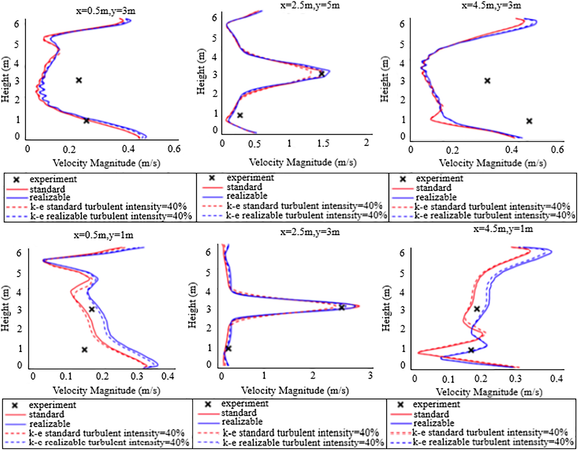
Figure 9: Vertical velocity profiles at different locations
The velocity profiles at the line which x = 2.5 m, y = 3 m and the line which x = 2.5 m, y = 5 m agree well with the experiment. For both the standard k-ε model and the realizable k-ε model, improving the intensity at the inlet can lower the velocity magnitude on the centreline of the jet. This effect is more notable for the standard k-ε model. The openings in the experiments are grilles, while in the model we simplified them to round openings of which the areas are equal to the effective area in the experiment. Improving the turbulent intensity can compensate for this simplification. When the turbulent intensity of the inlet is 40%, the realizable k-ε model shows a smaller decay on the jet, which is more in accordance with the experimental results.
For the measurement points at the line which x = 0.5 m, y = 3 m and the line which x = 4.5 m, y = 3 m, the velocity magnitudes are underestimated by both the standard k-ε model and the realizable k-ε model. The effect of the turbulent intensity at the inlet is not notable outside the jet. For the measurement points at the line which x = 0.5 m, y = 1 m and the line which x = 4.5 m, y = 1 m, the realizable k-ε model gives a higher prediction than the standard k-ε model. The realizable model fits better with the experimental data.
Generally, the realizable k-ε model and a turbulent intensity of 40% at the inlet predicts the velocity field most accurately.
Fig. 10 compares the simulated transient concentrations at several locations with the experimental data when Sct is set to the default of 0.7. For P1, P3, P6, P9, and P10, the simulation results fit the experimental data well. For P7, P8, P11, P12, P14, and P16, the predicted concentrations are higher than the experimental results. The positions where the concentration is overestimated in Fig. 10 are also where the velocity is underestimated in Fig. 9, which means that the concentration is related to the local velocity. It also shows that the realizable k-ε model with the species transport model can predict the concentration distribution well.
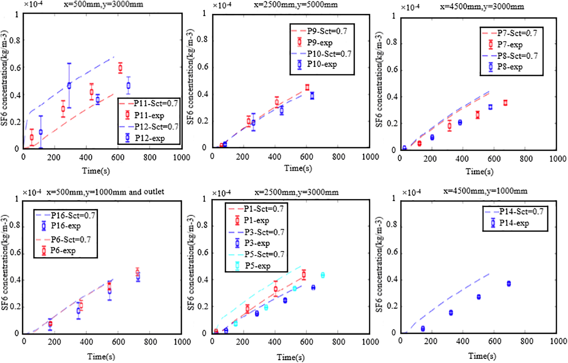
Figure 10: Transient concentration evolutions at different locations
4.2 Impact of Sct on Dimensionless Concentration Distribution
With the validated turbulence model and species transport model, we conducted three sets of simulations, as described in Section 3.4. As the emission rate changed in different simulation configurations, we needed a dimensionless concentration to judge the contaminant distribution. The dimensionless concentration Cstar is defined as
The dimensionless concentration is used in this section to judge the effect of Sct on the concentration distribution.
4.2.1 Contaminant Source of SF6 Released at 3 mL/s
Fig. 11 gives the dimensionless concentration at X = 0.5 m after 40 s of releasing SF6 at 3 mL/s. In this set of simulations, since the contaminant emission rate was low, the gravity seemed not affect the dispersion of SF6. The SF6 was influenced more by the flow in the space and moved upward. The area of iso-Cstar for each grade is the smallest when Sct = 0.4 and the largest when Sct = 1.
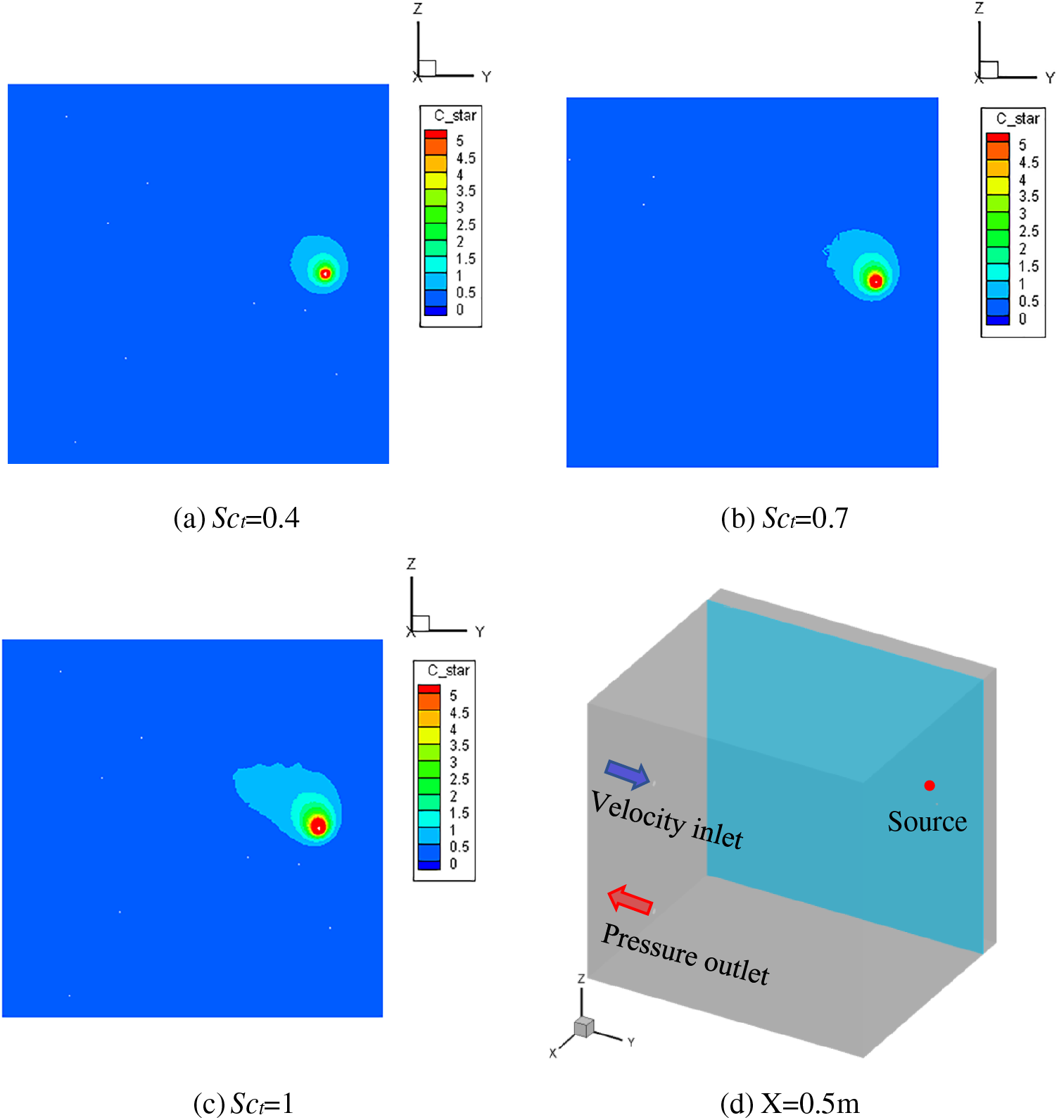
Figure 11: Dimensionless concentration at X = 0.5 m plane when sulfer hexafluoride has been released at low emission rate for 40 s
4.2.2 Contaminant Source of SF6 Released at 265.5 mL/s
Fig. 12 gives the dimensionless concentration at X = 0.5 m after 40 s of releasing SF6 at 265.5 mL/s. In this set of simulations, since the contaminant emission rate is high, the. The dispersion of SF6 around the source was more influenced by the gravitational force and moved downward. The area of iso-Cstar for each grade is the smallest when Sct = 0.4 and the largest when Sct = 1.
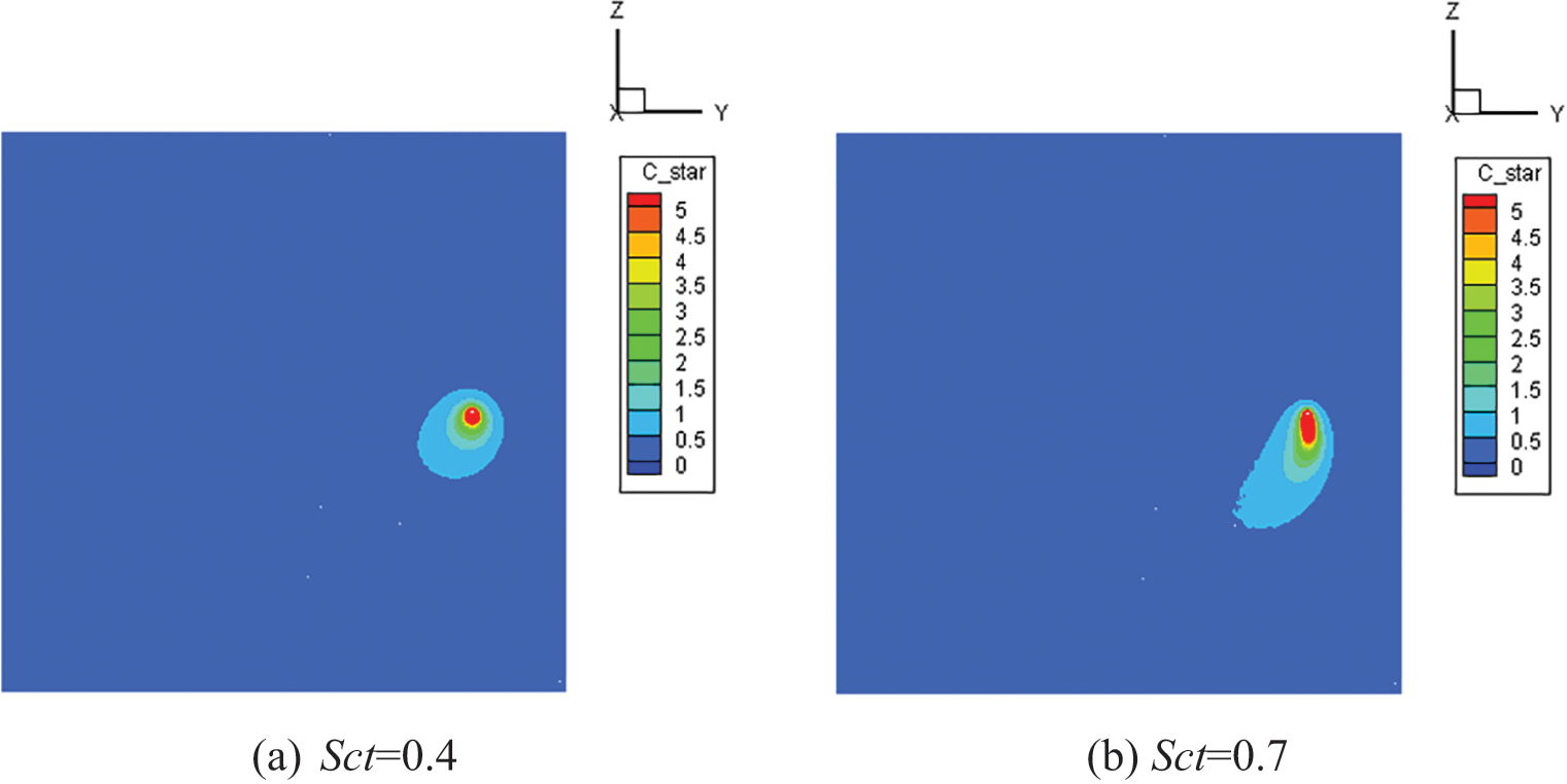
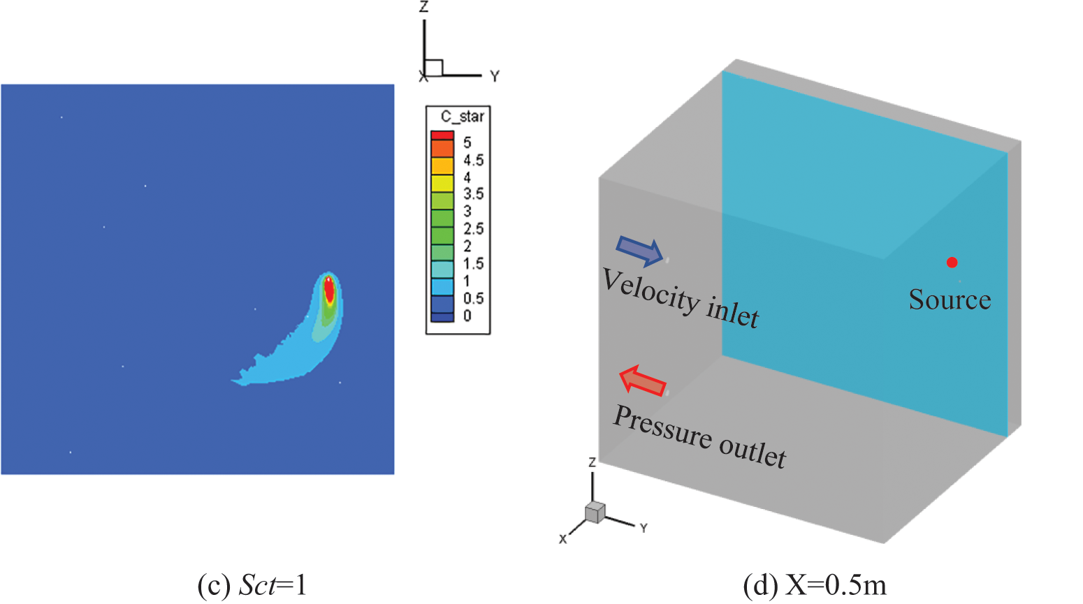
Figure 12: Dimensionless concentration at X = 0.5 m when sulfer hexafluoride has been released at a high emission rate for 40 s
Comparing Figs. 11 and 12, one can see that, although the emission rate differs, the effect of Sct is identical: the increase of Sct accelerates the contaminant transportation.
4.2.3 Contaminant Source of H2 Released at 265.5 mL/s
Fig. 13 gives the dimensionless concentration at X = 0.5 m after 40 s of releasing H2 at 265.5 mL/s. In this set of simulations, the low density of H2 took effect. The H2 concentration around the source was more influenced by the buoyancy and moved downward. The area of iso-Cstar for each grade is the largest when Sct = 0.4 and the smallest when Sct =1. For H2, the increase of Sct decelerates contaminant transportation. Comparing Figs. 12 and 13, we can conclude that different contaminant gases have different effects on the Sct, so it is not very rigorous to set it to a fixed value in the transient simulation.
Figure 13: Dimensionless concentration at X = 0.5 m plane when hydrogen has been released at low emission rate for 40 s
In summary, we can find that the effect of Sct on gas dispersion is different for different densities of gases, for higher density gases such as SF6, the gas dispersion rate is positively related to Sct; on the contrary, for lower density gases such as H2, the gas dispersion rate is negatively related to Sct. So for the indoor contaminant, the higher the density of the gas, we have to choose a lower Sct; for the lower density of the gas, we have to choose a higher Sct.
It can be seen that Sct is important for gas pollutant diffusion simulation. A default value cannot fit every gas pollutant. More in-depth studies are needed on Sct for diffusion simulation of other different gases, even ultra-fine particulate matter and bio-aerosols, etc.
To study the influence of Schmidt number on contaminant gas dispersion, we adopted a validated CFD model, which include the realizable k-ε turbulent model and a turbulent intensity of 40% at the inlet, to predict flow field and concentration of contaminant gas. And following conclusions were obtained.
For SF6 as the contaminant gas, the emission rate completely changed the concentration distribution. When the emission rate was low, the gravitational effect did not take place.
For both low and high emission rates, improving Sct accelerated the transportation of the SF6.
For H2 as the contaminant gas, improving Sct decelerated the transportation of the H2, which is the opposite of the pattern for SF6. So for the research subjects SF6 and H2 chosen in this paper, SF6 is more suitable for Sct = 0.4, choosing the smallest possible Sct; H2 is more suitable for Sct = 1, choosing the largest possible Sct. The Sct applicable to the diffusion simulation of different gases is worthy of further study.
Acknowledgement: None.
Funding Statement: This research were funded by the National Natural Science Foundation of China and the Machinery Industry Innovation Platform Construction Project of China Machinery Industry Federation, Grant Numbers 52378103 and 2019SA-10-07.
Author Contributions: The authors confirm contribution to the paper as follows: study conception and design: F.W. and Q.Z.; data collection: J.Z.; analysis and interpretation of results: X.W. and Y.L.; draft manuscript preparation: Q.M. and F.W. All authors reviewed the results and approved the final version of the manuscript.
Availability of Data and Materials: The data used in the study are available from corresponding author, please contact zhangqianru@usst.edu.cn.
Conflicts of Interest: The authors declare that they have no conflicts of interest to report regarding the present study.
References
1. Mazzola, T., Hanna, S., Chang, J. (2021). Results of comparisons of the predictions of 17 dense gas dispersion models with observations from the Jack Rabbit II chlorine field experiment. Atmospheric Environment, 244, 117887. https://doi.org/10.1016/j.atmosenv.2020.117887 [Google Scholar] [CrossRef]
2. He, J. X., Liu, L., Li, A. G., Ma, Y., Zhou, D. M. (2021). A dense gas dispersion model based on revised meteorological parameters and its performance evaluation. Atmospheric Environment, 244, 117953. https://doi.org/10.1016/j.atmosenv.2020.117953 [Google Scholar] [CrossRef]
3. Turner, D. B. (2020). Workbook of atmospheric dispersion estimates: An introduction to dispersion modeling. USA: CRC Press. [Google Scholar]
4. Weil, J. C., Alessandrini, S. (2023). The integral dense-gas dispersion model (IDDM) and comparison with Jack Rabbit II data. Atmospheric Environment, 296, 119563. https://doi.org/10.1016/j.atmosenv.2022.119563 [Google Scholar] [CrossRef]
5. Siddiqui, M., Jayanti, S., Swaminathan, T. (2012). CFD analysis of dense gas dispersion in indoor environment for risk assessment and risk mitigation. Journal of Hazardous Materials, 209, 177–185. [Google Scholar] [PubMed]
6. Rutkowski, D. R., Roldán-Alzate, A., Johnson, K. M. (2021). Enhancement of cerebrovascular 4D flow MRI velocity fields using machine learning and computational fluid dynamics simulation data. Scientific Reports, 11, 10240. https://doi.org/10.1038/s41598-021-89636-z [Google Scholar] [PubMed] [CrossRef]
7. Spalding, D. (1971). Concentration fluctuations in a round turbulent free jet. Chemical Engineering Science, 26, 95–107. [Google Scholar]
8. Bady, M., Kato, S., Huang, H. (2008). Towards the application of indoor ventilation efficiency indices to evaluate the air quality of urban areas. Building and Environment, 43(12), 1991–2004. https://doi.org/10.1016/j.buildenv.2007.11.013 [Google Scholar] [CrossRef]
9. Tahmooresi, S., Ahmadyar, D. (2021). Effects of turbulent Schmidt number on CFD simulation of 45° inclined negatively buoyant jets. Environmental Fluid Mechanics, 21, 39–62. https://doi.org/10.1007/s10652-020-09762-6 [Google Scholar] [CrossRef]
10. Balestrin, E., Souza, S. M. A. G. U. D., Valle, J. A. B. (2021). Sensitivity of the turbulent Schmidt number and the turbulence models to simulate catalytic and photocatalytic processes with surface reaction limited by mass transfer. Chemical Engineering Research and Design, 170, 90–106. https://doi.org/10.1016/j.cherd.2021.03.035 [Google Scholar] [CrossRef]
11. Blázquez, J. L. F., Maestre, I. R. (2023). Experimental adjustment of the turbulent Schmidt number to model the evaporation rate of swimming pools in CFD programmes. Case Studies in Thermal Engineering, 41, 102665. https://doi.org/10.1016/j.csite.2022.102665 [Google Scholar] [CrossRef]
12. Abe, S., Studer, E., Ishigaki, M. (2020). Density stratification breakup by a vertical jet: Experimental and numerical investigation on the effect of dynamic change of turbulent schmidt number. Nuclear Engineering and Design, 368, 110785. https://doi.org/10.1016/j.nucengdes.2020.110785 [Google Scholar] [CrossRef]
13. Chowdhury, M. N., Aziz, S. (2021). Effects of turbulence modeling and turbulent Schmidt number on supersonic mixing simulations. ASME International Mechanical Engineering Congress and Exposition. https://doi.org/10.1115/IMECE2021-69458 [Google Scholar] [CrossRef]
14. Koeltzsch, K. (2000). The height dependence of the turbulent Schmidt number within the boundary layer. Atmospheric Environment, 34(7), 1147–1151. [Google Scholar]
15. Tominaga, Y., Stathopoulos, T. (2007). Turbulent Schmidt numbers for CFD analysis with various types of flowfield. Atmospheric Environment, 41(37), 8091–8099. [Google Scholar]
16. He, G., Guo, Y., Hsu, A. T. (1999). The effect of Schmidt number on turbulent scalar mixing in a jet-in-crossflow. International Journal of Heat and Mass Transfer, 42(20), 3727–3738. [Google Scholar]
17. Kamotani, Y., Greber, I. (1972). Experiments on a turbulent jet in a cross flow. AIAA Journal, 10(11), 1425–1429. [Google Scholar]
18. Gromke, C., Blocken, B. (2015). Influence of avenue-trees on air quality at the urban neighborhood scale. Part I: Quality assurance studies and turbulent Schmidt number analysis for RANS CFD simulations. Environmental Pollution, 196, 214–223. https://doi.org/10.1016/j.envpol.2014.10.016 [Google Scholar] [PubMed] [CrossRef]
19. Nagaosa, R. S. (2014). A new numerical formulation of gas leakage and spread into a residential space in terms of hazard analysis. Journal of Hazardous Materials, 271, 266–274. [Google Scholar] [PubMed]
20. Cao, S. J., Meyers, J. (2013). Influence of turbulent boundary conditions on RANS simulations of pollutant dispersion in mechanically ventilated enclosures with transitional slot Reynolds number. Building and Environment, 59, 397–407. [Google Scholar]
21. Dong, L. X., Zuo, H. C., Hu, L., Yang, B., Li, L. C. et al. (2017). Simulation of heavy gas dispersion in a large indoor space using CFD model. Journal of Loss Prevention in the Process Industries, 46, 1–12. https://doi.org/10.1016/j.jip.2017.01.012 [Google Scholar] [CrossRef]
22. Marquardt, P., Klaas, M., Schröder, W. (2020). Experimental investigation of the turbulent Schmidt number in supersonic film cooling with shock interaction. Experiments in Fluids, 61, 160. https://doi.org/10.1007/s00348-020-02983-x [Google Scholar] [CrossRef]
23. Shi, Z., Chen, J., Chen, Q. Y. (2016). On the turbulence models and turbulent Schmidt number in simulating stratified flows. Journal of Building Performance Simulation, 9(2), 134–148. [Google Scholar]
24. Li, F., Liu, J. J., Ren, J. L., Cao, X. D. (2018). Predicting contaminant dispersion using modified turbulent Schmidt numbers from different vortex structures. Building and Environment, 130, 120–127. [Google Scholar] [PubMed]
25. Zhang, Q., Zhang, X., Ye, W., Liu, L., Nielsen, P. V. (2018). Experimental study of dense gas contaminant transport characteristics in a large space chamber. Building and Environment, 138, 98–105. [Google Scholar]
26. Deng, B. C., Shin, Y. J., Lu, L., Zhang, Z. Q., Karniadakis, G. E. (2022). Approximation rates of DeepONets for learning operators arising from advection-diffusion equations. Neural Networks, 153, 411–426. https://doi.org/10.1016/j.neunet.2022.06.019 [Google Scholar] [PubMed] [CrossRef]
27. Jena, S. R., Gebremedhin, G. S. (2021). Computational technique for heat and advection—diffusion equations. Soft Computing, 25, 11139–11150. https://doi.org/10.1007/s00500-021-05859-2 [Google Scholar] [CrossRef]
28. Fluent, A. (2023). 2023R1 theory guide. USA: Ansys Inc. [Google Scholar]
29. Fluent, A. (2023). 2023R1 user’s guide. USA: Ansys Inc. [Google Scholar]
Cite This Article
 Copyright © 2024 The Author(s). Published by Tech Science Press.
This work is licensed under a Creative Commons Attribution 4.0 International License , which permits unrestricted use, distribution, and reproduction in any medium, provided the original work is properly cited.
 Downloads
 Citation Tools