Formation of Water Quality of Surface Water Bodies Used in the Material Processing

Nomenclature

1  Introduction

Mergers are the most important nodes of the river network. Understanding the mechanism of pollutant transport at the confluence of rivers is critical for assessing water quality. It is proved that any differences in the characteristics of tributary water (for example, temperature, and concentration of suspended particles) can cause stratification of waters [1–4]. Within the framework of these studies, the mechanisms of the confluence of the Kama and Vishera rivers, below which the water supply of large industrial enterprises of the Solikamsk-Berezniki industrial complex is located downstream, have been studied. Assessing the intensity of mixing of merging rivers is of both theoretical and practical interest related to the construction of schemes for the most rational use of water resources. In the last 20–30 years, the interest in this topic has increased significantly due to the wide availability of images of good resolution of river confluence zones. A completely natural question arises: why for some rivers mixing occurs very intensively, and for others very slowly, while significant differences are also observed according to the seasons of the year. The literature offers various explanations for this phenomenon. In the works of [3,4], a hypothesis on the connection of this phenomenon with secondary circulation is suggested and verified. The present work examines the influence of various factors (merging angle, flow rate ratio) on secondary circulation and mixing intensity.

In recent years, thanks to the data from satellite images, the interest of researchers in the phenomenon of “non-mixing” of rivers has increased. The width of the river mixing zone is not always proportional to the total width of the merging rivers. Sometimes it is several dozen times larger than the width of the tributaries [5–7]. Theoretical analysis [8] has shown that the distance required for mixing in the downstream direction is proportional to the square of the width of the flow after merging. This dependence explains why large rivers take longer to mix than small ones. However, as the study [6] showed, the nature of the formation of transverse circulation may be of fundamental importance for the phenomenon of “non-mixing”. Transverse circulation, in turn, is determined by the nature and structure of secondary currents. Makkaveev in 1947 [9], based on the works of Schmidt 1917, 1926 [10], suggested that the mixing of waters in rivers occurs according to the scheme of Fick diffusion [11]. However, this scheme does not take into account the complex structure of currents in channel flows, which leads to anisotropy of diffusion. Taylor back in 1953 [12] found that the unevenness of the field of averaged flow velocities can greatly affect the nature of not only longitudinal, but also transverse diffusion. Prandtl et al. [13] showed that even in rectilinear sections, due to the uneven distribution of tangential stresses, secondary flows, called “secondary flows of the second kind”, can occur. The unevenness of tangential stresses is due to the non-circular shape of the bottom, the roughness of the bottom. Currents of the first kind arise when the direction of flow in the channel changes. Although the velocities of these currents are small and do not exceed 2%–3% of the velocity of the averaged longitudinal flow, their contribution is comparable to the contribution of turbulent pulsations [14,15].

Currently, there are several hypotheses explaining the occurrence of secondary vortices of the second kind. In [16], the occurrence of secondary flows is explained by the distribution of the average pressure in the cross section, or in other words, the balance of viscous friction forces and Reynolds stresses. Another explanation proposed in [17], reference [18] was based on the analysis of the terms of the kinetic energy balance equation of turbulent pulsations. If at some point in the flow the kinetic energy production is significantly greater than the viscous dissipation, then a secondary flow occurs, transferring liquid particles with greater kinetic energy from this region to the region where the energy production is less than the dissipation. An alternative mechanism for the occurrence of secondary vortices, proposed in [19], is that longitudinal vortices are formed under the action of turbulent pulsations, in which the pulsations of the longitudinal component of vorticity are specially phase-coordinated with the pulsations of the longitudinal component of velocity.

In the present paper, the area of confluence of the Kama and Vishera rivers is considered as an object of transverse circulation research. These rivers are characterized by fairly similar values of flow rates and water density. Due to the fact that the Kama River crosses a very large swamp massif before merging with the Vishera, the color of the water in the Kama is darker than in the Vishera, which is very clearly visible on satellite images (see Fig. 1). The confluence of the Vishera and Kama Rivers is located directly above the largest river in the basin. Volga mining complex of the Solikamsk-Berezniki industrial hub, developing one of the world’s largest Verkhnekamskoye deposit of potash and magnesium ores.

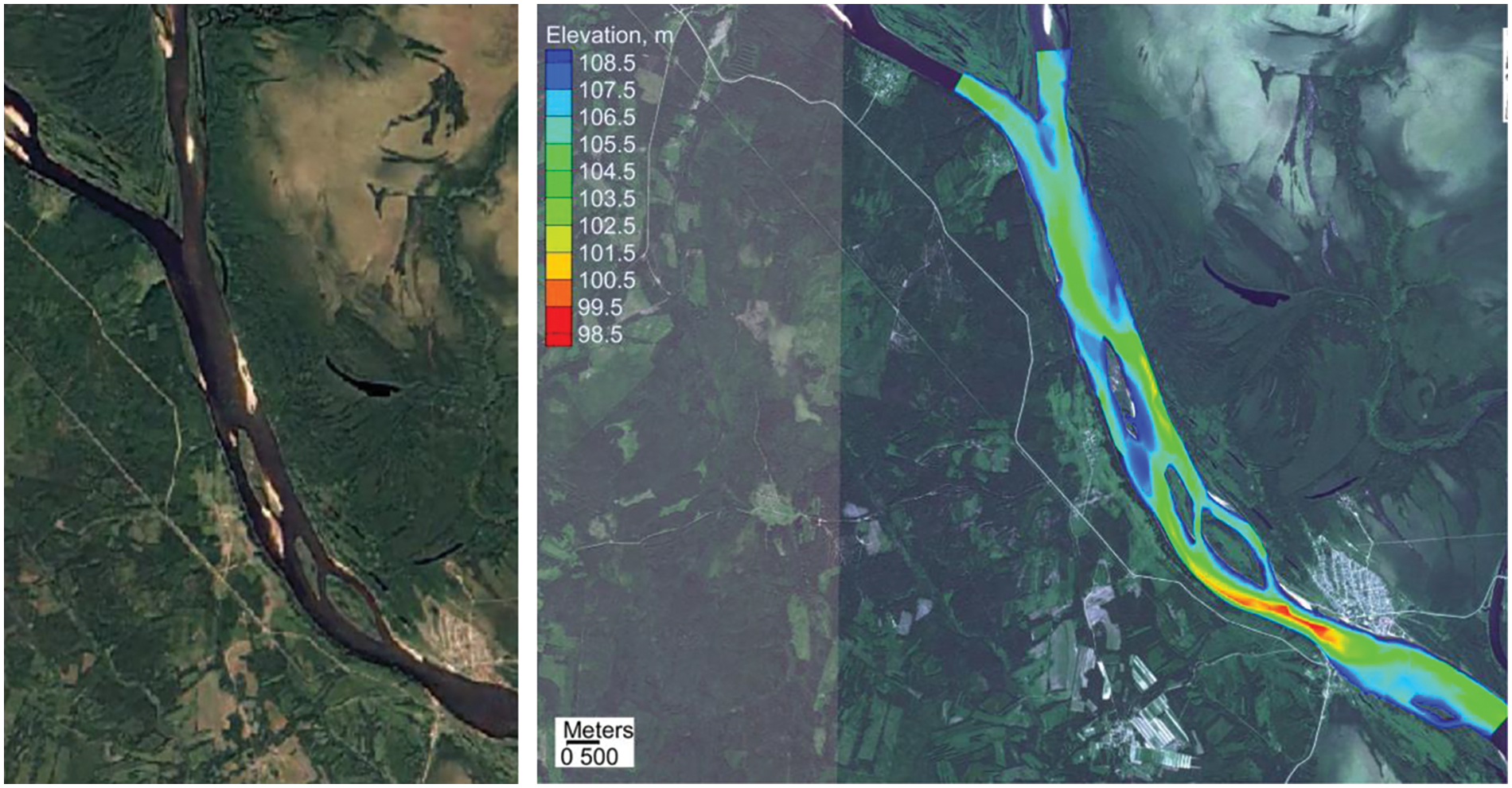
Figure 1: Aerial photographs of the confluence of the Kama (left) and Vishera (right) rivers

The confluence of rivers is a complex process that depends on such factors as the type of confluence (symmetrical, i.e., Y-shaped; asymmetric), the angle of confluence, the width and depth of the river, the slope of the riverbed, the flow rate, the direction of flow, the roughness of the bottom and the Froude number-the ratio between the force of inertia and the external force in the field which is moving [20]. In this paper, the calculation of the confluence of rivers in a model rectangular geometry is carried out. The use of model geometry is intended to eliminate other effects that affect fusion. The confluence of rivers at an angle of 0 degrees is also considered, in other words, the flow in the channel. It is assumed that in such a configuration, there are no flows of the first kind according to Prandtl. The vast majority of theoretical and experimental works [21–25] devoted to the confluence of rivers consider small (the ratio of width to depth W/H is less than 10) and medium-sized rivers (10 < W/H < 50). This selective interest of researchers is due to natural features: most of the rivers are small or large. This paper considers the confluence of large rivers (W/H > 50). Calculations were carried out on the basis of the RANS turbulence model, which includes seven equations [26–29]. The results are presented for a model confluence of rivers at an angle of 0, 30, 45, and 60 degrees. For a confluence close to real conditions (45 degrees), 2 models were calculated, differing in the rate of inflows: 0.5 and 0.6 m/s. Graphs of the mixing zone width, the maximum vorticity value, concentration fields, and vorticity contours for various cross sections after the confluence site are obtained.

2  Problem Statement

2.1 Geometry and Grid

To clarify the mechanism of mixing flows in the confluence of rivers, calculations were carried out for a model configuration in the case of two rivers characterized by the same spatial dimensions as the Kama and Vishera rivers, but with rectilinear sections of the channel and constant depth (see Fig. 2).

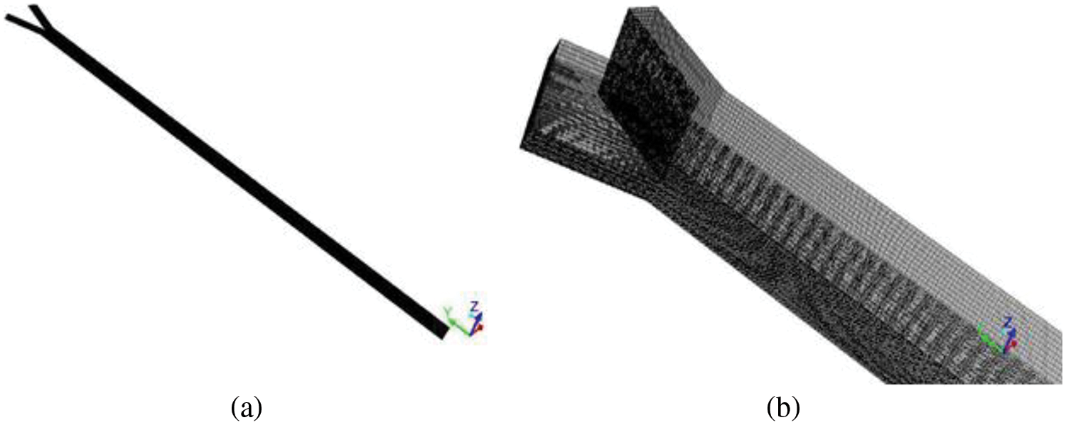
Figure 2: (a) geometry of the problem; (b) calculation grid

Calculations were carried out for a section of 11 km in length. The estimated area included sections of rivers with a length of 500 m to the confluence, and a section with a length of 10 km downstream from the confluence. The width of the riverbeds to the confluence was considered to be the same and equal to 250 m, the width of the riverbed flowing from the confluence was assumed to be equal to 500 m. The depth of the rivers was assumed to be the same, constant and equal to 8 m in the entire area under consideration. Calculation grid (see Fig. 2) in the horizontal direction consisted of quadrangular cells with a characteristic linear size of 10 m, evenly distributed along the entire length, vertically 0.1 m. The total number of grid nodes was 4,800,000.

2.2 Governing Equations

The equation of mass and momentum balance for the Reynolds averaged velocity has the form:

∂ρ∂t+∂∂xi(ρvi)=0, (1)

∂∂t(ρvi)+∂∂xj(ρvivj)=−∂p∂xi+∂∂xj[μ(∂vi∂xj+∂vj∂xi−23δij∂vl∂xl)]

+∂∂xj[μt(∂vi∂xj+∂vj∂xi)−23(ρk+μt∂vl∂xl)δij]+ρgi. (2)

Eqs. (1) and (2) contain the following notation: ρ this is the density of the liquid, vi the components of the averaged velocity ( i=x,y,z -Cartesian coordinates), p is the pressure, μ the dynamic viscosity of the liquid, δij —the Kronecker symbol. The turbulent viscosity μt is a function of the turbulent kinetic energy k and ε its dissipation rate μt=ρCμk2/ε : empirical constant Cμ=0.09 [30].

Closure equations for Reynolds stress:

∂∂t(ρv′iv′j¯)+∂∂xk(ρvkv′iv′j¯)=∂∂xk(μtσk∂v′iv′j¯∂xk)+∂∂xk[μ∂∂xk(v′iv′j¯)]−ρ(v′iv′k¯∂vj∂xk+v′jv′k¯∂vi∂xk)−C1ρεk(v′iv′j¯−23δijk)+23δijρε, (3)

where C1=1.8 is the empirical constant [30].

Here the turbulent kinetic energy is defined as k=12v′iv′i . To obtain boundary conditions for Reynolds stresses, it is necessary to solve the equation of turbulent kinetic energy transfer:

∂∂t(ρk)+∂∂xi(ρkvi)=∂∂xj((μ+μtσk)∂k∂xi)+12ρ(v′iv′k¯∂vi∂xk+v′iv′k¯∂vi∂xk)+Gk+Gb−ρε. (4)

Here σk=0.82 .

The dissipation rate is calculated using the model transfer equation:

∂∂t(ρε)+∂∂xi(ρεvi)=∂∂xj((μ+μtσε)∂ε∂xj)+Cε112ρ(v′iv′k¯∂vi∂xk+v′iv′k¯∂vi∂xk)+C1εεkGk−C2ερε2k, (5)

where Cε1=1.44 , σε=1.0 , Cε2=1.92 .

In Eqs. (4) and (5), the following notations are introduced: Gk=μtS2 is the generation of turbulent kinetic energy due to the average velocity gradient; S=2SijSij is the norm of the tensor of the average flow strain rate, Sij=12(∂vj∂xi+∂vi∂xj) Gb=−gj(μt/ρ)Prt∂ρ∂xj is the generation of turbulent energy due to buoyancy force in the gravity field.

The impurity transport equation is written as

∂∂t(ρc)+∇⋅(ρvc)=−∇⋅J. (6)

Eq. (6) contains the following notation: с is the impurity concentration (wt%-weight percent, concentration varies from 0 to 1), ∇ is the nabla operator; J is the vector of the diffusion flux of the impurity, defined by the expression:

J=−ρ(Dm+Dt)∇c, (7)

where Dm is the molecular diffusion coefficient, Dt is the effective turbulent diffusion coefficient associated with the turbulent viscosity μt ratio Dt=(μt/ρ)/Sct , here Sct is the turbulent Schmidt number. Impurity is a passive scalar introduced for the description.

Parameters used in Eqs. (1)–(7), Prt , Sct , G1ε , C2ε , σk , and σε are empirical constants and their values were taken from [30], some of them are given earlier in the text, Prt=0.85 , Sct=0.7 . The kinematic viscosity was assumed to be μ=9.34⋅10−7 m2/s, the molecular diffusion coefficient Dm=1.0⋅10−9 m2/s. The second-order accuracy scheme was used to perform spatial discretization of equations.

The boundary conditions for Eqs. (1)–(7) are given below for different boundaries of the system. The condition of adhesion and the condition of zero mass flow on solid boundaries (bottom and river banks) were imposed:

vx=vy=vz=0. (8)

The boundary conditions for the values of Reynolds stresses on solid walls are calculated from the wall functions. Wall functions are introduced in accordance with the work [16], they are most widely used for modeling natural flows.

The wall function for the average velocity has the form:

U∗=1κln⁡(Ey∗). (9)

Here U∗=UPCμ1/4kP1/2τw/ρ , y∗=ρCμ1/4kP1/2yPμ , κ=0.4187 is the Karman constant, E=9.793 is the empirical constant, the UP is the average velocity of the fluid at the point P , kP is the the turbulent kinetic energy at the point P , yP is the distance from the point P to the wall.

The logarithmic law (9) applies when 11.225<y∗<300 . When the grid is such that in the cells adjacent to the wall y∗<11.225 , Eq. (9) has the form U∗=y∗ .

The Reynolds stresses in the cells adjacent to the wall are calculated using the formulas:

v′i2¯k=1.098,  v′j2¯k=0.247,  v′k2¯k=0.655,  −v′iv′j¯k=0.255

For the impurity, the law near the wall has the form:

(cw−c)ρCμ1/4kP1/2Jw={Scy∗                          (y∗<yc∗)Sct[1κln⁡(Ey∗)+Pc]    (y∗>yc∗),

where both the molecular and turbulent Schmidt numbers define the diffusion flux of the impurity on the wall. The index w stands for “wall”.

Pc=9.24[(ScSct)3/4−1] [1+0.28e−0.007Sc/Sct]

Eq. (2) for k is solved in the entire area, including the cells adjacent to the wall. Boundary condition for k on the wall:

∂k∂n=0,

where k is the coordinate normal to the wall.

The production of kinetic energy and the rate of its dissipation in the cells adjacent to the wall, which are the initial terms in the equation, are calculated based on the hypothesis of local equilibrium. Under this assumption, it is assumed that the production and the rate of energy dissipation in the control volume adjacent to the wall are equal.

Thus, production is calculated from:

Gk≈τw∂U∂y=τwτwκρCμ1/4kP1/2yP

The dissipation rate is calculated by the formula: ε=Cμ3/4kP3/2κyP .

At the entrance to the computational domain, the velocity of the main stream was prescribed (the vector of the flow velocity of the environment is perpendicular to the input boundary U→={U, 0, 0} ); the concentration was set equal to the background concentration of the impurity in the water for each river its own:

vx=U,vy=0,vz=0,c=c0. (10)

The Reynolds stresses at the input are calculated from the assumption of turbulence isotropy:

v′i2¯=23k,   v′iv′j¯=0.0.

Here k=32(vavgI)2 vavg the average flow velocity, turbulence intensity I=0.16Re−1/8 .

The upper boundary of the region corresponding to the free surface of the liquid was assumed to be undeformable; the conditions for the absence of a normal component of velocity, tangential stresses and impurity flow were considered fulfilled on it:

(vn)=0,∂vx∂xz+∂vz∂xx=0,∂vy∂xz+∂vz∂xy=0,∂c∂n=0 (11)

The conditions at the output of the computational domain consisted in the fulfillment of the mass balance condition:

∮SinρvindS−∮SoutρvoutdS=0

3  Numerical Results

3.1 Features of the Hydrodynamics of the Confluence of Rivers at a Confluence Angle of 45°

Fig. 3 shows the fields of impurity concentration and flow vorticity in the cross sections of the channel located at different distances from the confluence (0, 1000 m, etc.) for the same velocities of merging rivers equal to 0.5 m/s. The color scale corresponds to the impurity concentration indicators. The gray lines show the flow vorticity isolines (x-components of the velocity rotor). As can be seen from the graphs, there is an increase in the width of the mixing zone and a decrease in vorticity with distance from the confluence site. The secondary flow is two vortices of different directions.

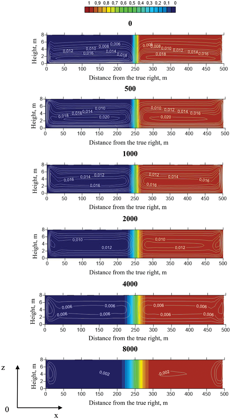
Figure 3: Concentration and vorticity fields for the inflow velocity of 0.5 m/s, confluence angle 45°

Based on the results of calculations, the width of the mixing zone was calculated. This characteristic was defined as the doubled difference between the coordinates of the point at which the concentration is 0.5 (the middle of the horizontal cross-section y = 250 m) and the point at which the concentration value differs from zero by 10−4. Fig. 4 shows the dependence of the mixing zone width on the distance from the confluence point. As can be seen from the figure, the width of the mixing zone increases with distance from the confluence, especially a sharp increase is observed in the first thousand meters.

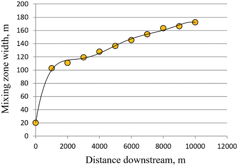
Figure 4: The dependence of the size of the mixing zone on the distance after the confluence point for an angle of 45°

3.2 Influence of the Velocities of Merging Rivers

Fig. 5 shows the fields of impurity concentration and flow vorticity in the cross sections of the channel located at different distances from the confluence (0, 1000 m, etc.) for the same velocities of merging rivers equal to 0.6 m/s. As can be seen from the comparison with Figs. 3 and 5, with an increase in the velocity of merging rivers, the secondary vorticity of the flow increases. Secondary vortices are realized across the channel, the main flow is observed along the channel, while the intensity of secondary flows.

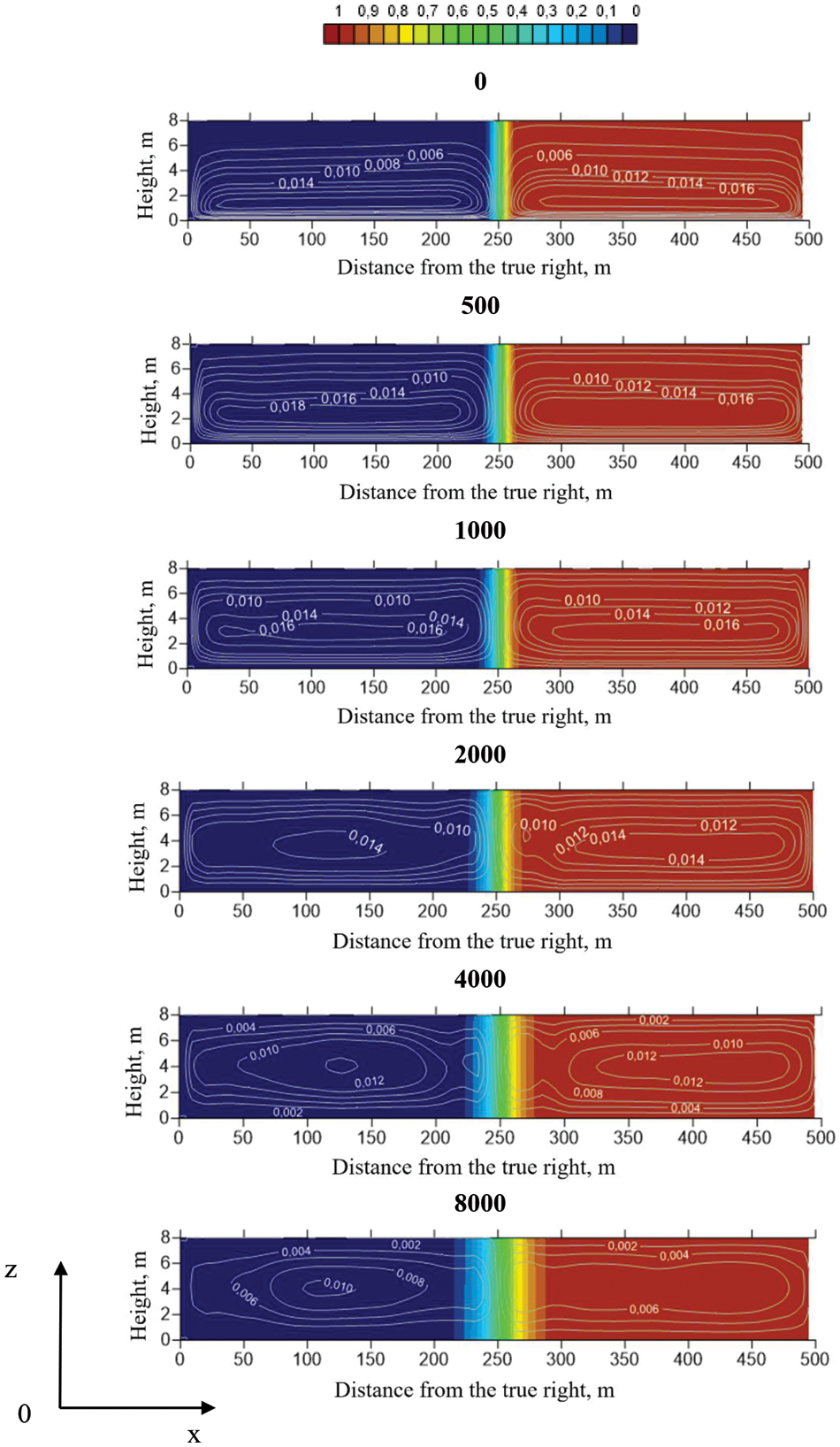
Figure 5: Concentration and vorticity fields for the inflow velocity of 0.6 m/s, confluence angle of 45°

For two cases, the input velocity differs by 20%, while the maximum value of vorticity for these variants correspondingly differs by 13% (Fig. 6).

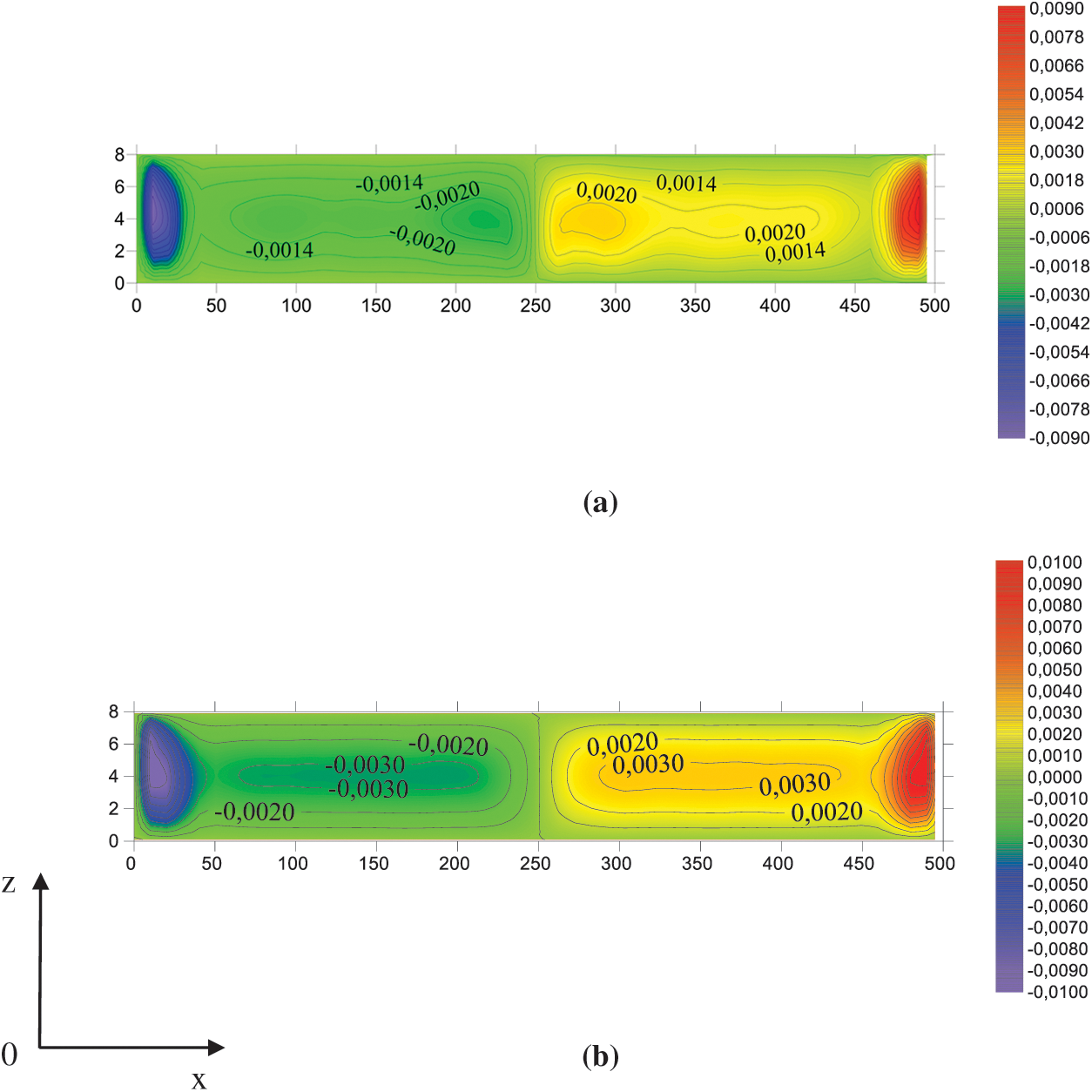
Figure 6: The field of vorticity in the vertical section at a distance of 8000 m from the confluence. The velocity at the input of the computational domain is constant, equal to (a) 0.5 m/s, (b) 0.6 m/s

This result is also illustrated by Fig. 7, which shows the dependences of the vorticity of the flow with the distance from the confluence for two flow velocities of merging rivers: 0.5 and 0.6 m/s.

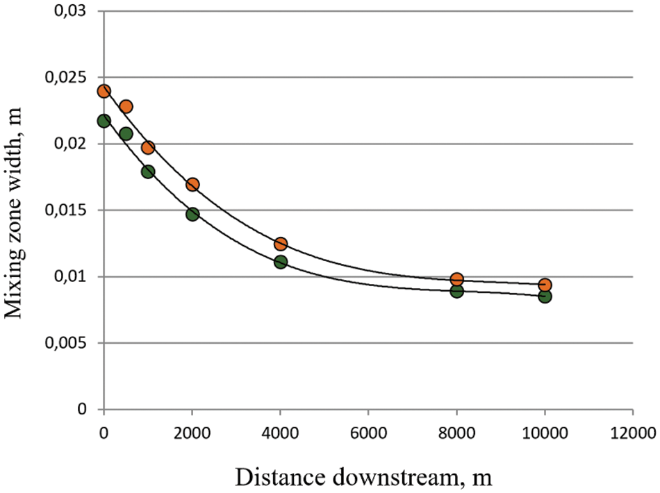
Figure 7: The dependence of the maximum vorticity value on the distance downstream from the confluence for an angle of 45° for the average speed of the main flow in the channels, 0.5 m/s (orange) and 0.6 m/s (green)

3.3 Influence of the Angle of Confluence of Rivers

The intensity of secondary currents depends on the angle of the intersection of channels. To study the changes in the intensity and structure of the secondary circulation from the angle of fusion, a series of calculations were carried out for the cases of 0°, 30°, 45°, and 60°. A graph of the concentration change from 0 to 1 wt% with a distance from the left bank is shown in Fig. 8. The graph is plotted for a section located at a distance of 8000 m from the confluence. The concentration scale is presented on a logarithmic scale to visualize changes in concentration on a horizontal scale. With an increase in the angle of fusion, the width of the zone in which the concentration change increases.

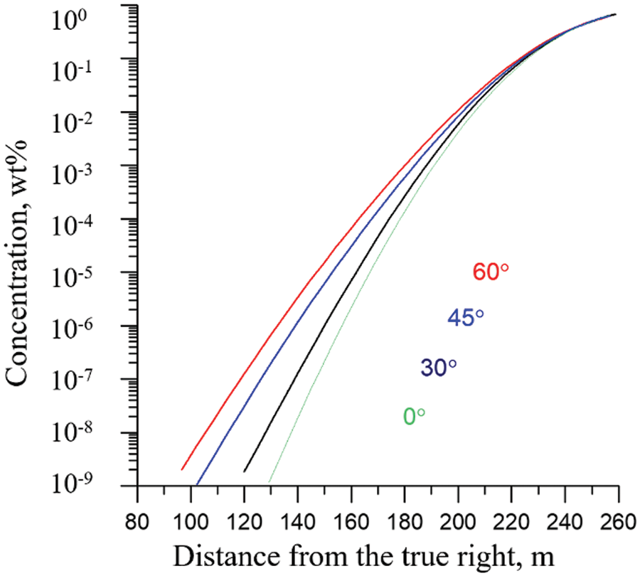
Figure 8: Graph of changes in the concentration of passive impurity with a change in the angle of channel fusion: 0°, 30°, 45°, 60°

Fig. 9 shows the dependence of the mixing zone width on the distance from the confluence site for 4 different confluence angles at a flow velocity of 0.5 m/s. As can be seen, the width of the mixing zone increases with the increase in the angle of fusion. In all cases, except for the angle of 0°, there is a sharp increase in the width of the mixing zone in the initial section.

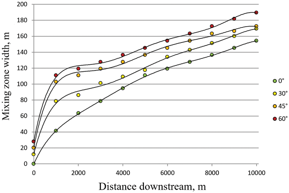
Figure 9: Dependence of the displacement zone size on the distance after the confluence point for different angles of confluence

Fig. 10 shows the vorticity fields at distances of 1000 and 8000 m from the confluence point for a confluence angle of 0°. As can be seen in this case, there are only fairly intense vortices at the lateral boundaries of the computational domain (river banks). In the rest of the region, the vorticity is close to zero.

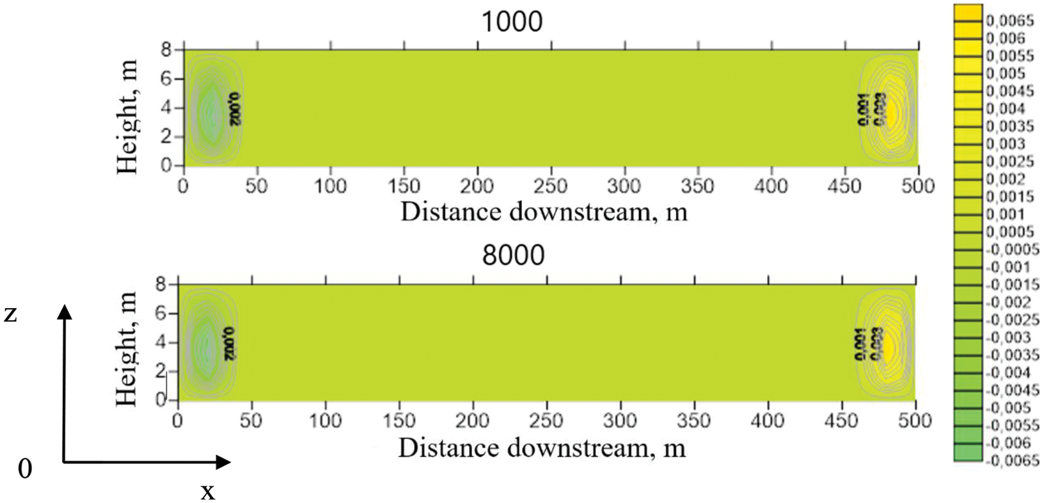
Figure 10: Vorticity of the flow in the channel

4  Conclusion

The hydrodynamic aspects of the confluence of the Kama and Vishera rivers are numerically investigated. The fields of concentration of passive impurity and vorticity, as well as the width of the mixing zone depending on the distance from the confluence, the velocities of the merging rivers and the angle of confluence are obtained.

It is found that:

1) the width of the mixing zone increases with distance from the confluence site, especially a sharp increase is observed at non-zero fusion angles;

2) as the velocity of merging rivers increases, the vorticity of the current increases;

3) as the angle of fusion increases, the width of the mixing zone increases. The slope of the initial section of the curve also increases with the increase in the angle of fusion;

4) at a confluence angle of 0°, there are only fairly intense vortices at the lateral boundaries of the computational domain (river banks). In the rest of the region, the vorticity is close to zero.

Specific values of hydrochemical and physical indicators of water quality are stochastic in nature, the dispersion of which is determined primarily by the variability of hydrological indicators of merging rivers, therefore calculations were carried out for some characteristic model conditions for which detailed measurements were performed. Therefore, it is not correct to consider the obtained estimates as some typical average annual or even seasonal values. At the same time, due to the remoteness of the research area and the undeveloped territory, it is not possible to conduct field surveys with a significant frequency of observations. Despite some “model nature” of the results obtained, they are of fundamental importance for the formation of programs for further field studies. In particular, due to the labor-intensive nature of field study implementation, it is necessary to make the most efficient use of the combination of field studies and computational experiments.

Acknowledgement: None.

Funding Statement: The study was carried out with financial support from the Government of the Perm Territory within the Framework of Scientific Project No. S-26/828 and the Ministry of Science and High Education of Russia (Theme No. 121031700169-1).

Author Contributions: The authors confirm contribution to the paper as follows: study conception and design: T. Lyubimova, A. Lepikhin; performing calculations: Y. Parshakova, I. Zayakina; analysis and interpretation of results: T. Lyubimova, A. Lepikhin. A. Issakhov; draft manuscript preparation: T. Lyubimova, Y. Parshakova. All authors reviewed the results and approved the final version of the manuscript.

Availability of Data and Materials: The data that support the findings of this study are available on request from the corresponding author.

Conflicts of Interest: The authors declare that they have no conflicts of interest to report regarding the present study.

References

1. Jiang, C., Constantinescu, G., Yuan, S., Tang, H. (2023). Flow hydrodynamics, density contrast effects and mixing at the confluence between the Yangtze River and the Poyang Lake channel. Environmental Fluid Mechanics, 23(2), 229–257. https://doi.org/10.1007/s10652-022-09848-3 [Google Scholar] [CrossRef]

2. Yuan, S. Y., Xu, L., Tang, H. W., Xiao, Y., Gualtieri, C. (2022). The dynamics of river confluences and their effects on the ecology of aquatic environment: A review. Journal of Hydrodynamics, 34(1), 1–14. https://doi.org/10.1007/s42241-022-0001-z [Google Scholar] [CrossRef]

3. Lyubimova, T. P., Lepikhin, A. P., Parshakova, Y. N., Kolchanov, V. Y., Gualtieri, C. et al. (2020). A numerical study of the influence of channel-scale secondary circulation on mixing processes downstream of river junctions. Water, 12(11), 2969. https://doi.org/10.3390/w12112969 [Google Scholar] [CrossRef]

4. Lyubimova, T. P., Lepikhin, A. P., Parshakova, Y. N., Kolchanov, V. Y., Gualtieri, C. et al. (2021). Hydrodynamic aspects of confluence of rivers with different water densities. Journal of Applied Mechanics and Technical Physics, 62(7), 1211–1221. https://doi.org/10.1134/S0021894421070130 [Google Scholar] [CrossRef]

5. Mackay, J. R. (1970). Lateral mixing of the liard and mackenzie rivers downstream from their confluence. Canadian Journal of Earth Sciences, 7(1), 111–124. https://doi.org/10.1139/E70-008 [Google Scholar] [CrossRef]

6. Lane, S. N., Parsons, D. R., Best, J. L., Orfeo, O., Kostaschuk, R. A. et al. (2008). Causes of rapid mixing at a junction of two large rivers: Río Paraná and Río Paraguay Argentina. Journal of Geophysical Research: Earth Surface, 113(F2). https://doi.org/10.1029/2006JF000745 [Google Scholar] [CrossRef]

7. Bouchez, J., Lajeunesse, E., Gaillardet, J., France-Lanord, C., Dutra-Maia, P. et al. (2010). Turbulent mixing in the amazon river: The isotopic memory of confluences. Earth and Planetary Science Letters, 290(1–2), 37–43. https://doi.org/10.1016/j.epsl.2009.11.054 [Google Scholar] [CrossRef]

8. Rutherford, J. C. (1994). River mixing. Hoboken, New Jersey, USA: Wiley. [Google Scholar]

9. Makkaveev, V. M. (1947). Distribution of longitudinal and transverse velocities in open flows. Proceedings of the State Hydrological Institute, pp. 3–36. [Google Scholar]

10. Schmidt, W. (1926). Der Massenaustausch in freier Luft und verwandte Erscheinungen, vol. 7. Hamburg, Germany: H. Grand. [Google Scholar]

11. Kerimova, S. A. (2011). Investigation of the propagation of pollutants in water reservoirs. Journal of Engineering Physics and Thermophysics, 84, 298–304. https://doi.org/10.1007/s10891-011-0473-0 [Google Scholar] [CrossRef]

12. Taylor, G. I. (1953). Dispersion of soluble matter in solvent flowing slowly through a tube. Proceedings of the Royal Society of London. Series A. Mathematical and Physical Sciences, 219(1137), 186–203. https://doi.org/10.1098/RSPA.1953.0139 [Google Scholar] [CrossRef]

13. Prandtl, L., Tietjens, O. G. (2011). Fundamentals of hydro and aeromechanics: dover. New York, USA: United Engineering Trusters Inc. [Google Scholar]

14. Nikuradse, J. (1930). Untersuchungen über turbulente Strömungen in nicht kreisförmigen Rohren. Ingenieur-Archiv, 1, 306–332. [Google Scholar]

15. Nikitin, N. V., Popelenskaya, N. V., Stroh, A. (2021). Prandtl’s secondary flows of the second kind. Problems of description, prediction, and simulation. Fluid Dynamics, 56(4), 513–538. https://doi.org/10.1134/S0015462821040091 [Google Scholar] [CrossRef]

16. Nikitin, N. (2021). Turbulent secondary flows in channels with no-slip and shear-free boundaries. Journal of Fluid Mechanics, 917, A24. https://doi.org/10.1017/jfm.2021.306 [Google Scholar] [CrossRef]

17. Hinze, J. O. (1967). Secondary currents in wall turbulence. The Physics of Fluids, 10(9), S122–S125. https://doi.org/10.1063/1.1762429 [Google Scholar] [CrossRef]

18. Hinze, J. O. (1973). Experimental investigation on secondary currents in the turbulent flow through a straight conduit. Applied Scientific Research, 28, 453–465. https://doi.org/10.1007/BF00413083/METRICS [Google Scholar] [CrossRef]

19. Nikitin, N. V., Pimanov, V. O., Popelenskaya, N. V. (2019). Mechanism of formation of Prandtl’s secondary flows of the second kind. In: Doklady physics, vol. 64, pp. 61–65. New York, USA: Pleiades Publishing. https://doi.org/10.1134/S1028335819020034 [Google Scholar] [CrossRef]

20. Biswal, S. K., Mohapatra, P. K., Muralidhar, K. (2012). Flow separation at an open channel confluence. ISH Journal of Hydraulic Engineering, 16, 89–98. https://doi.org/10.1080/09715010.2010.10515018 [Google Scholar] [CrossRef]

21. Bradbrook, K. F., Lane, S. N., Richards, K. S. (2000). Numerical simulation of three-dimensional, time-averaged flow structure at river channel confluences. Water Resources Research, 36(9), 2731–2746. https://doi.org/10.1029/2000WR900011 [Google Scholar] [CrossRef]

22. Zhang, Z., Lin, Y. (2021). An experimental study on the influence of drastically varying discharge ratios on bed topography and flow structure at urban channel confluences. Water, 13(9), 1147. https://doi.org/10.3390/w13091147 [Google Scholar] [CrossRef]

23. Sabrina, S., Lewis, Q., Rhoads, B. (2021). Large-scale particle image velocimetry reveals pulsing of incoming flow at a stream confluence. Water Resources Research, 57(9), e2021WR029662. https://doi.org/10.1029/2021WR029662 [Google Scholar] [CrossRef]

24. Leli, I. T., Stevaux, J. C., Bennert, A., dos Santos, V. C., Luz, L. D. (2023). Morphological resilience at the confluence of a very low discharge creek and a large river (upper Parana, Brazil). Journal of South American Earth Sciences, 123, 104222. https://doi.org/10.1016/j.jsames.2023.104222 [Google Scholar] [CrossRef]

25. Alizadeh, L., Fernandes, J. (2021). Turbulent flow structure in a confluence: Influence of tributaries width and discharge ratios. Water, 13(4), 465. https://doi.org/10.3390/w13040465 [Google Scholar] [CrossRef]

26. Shaheed, R., Yan, X., Mohammadian, A. (2021). Review and comparison of numerical simulations of secondary flow in river confluences. Water, 13(14), 1917. https://doi.org/10.3390/w13141917 [Google Scholar] [CrossRef]

27. Safarzadeh, A., Brevis, W. (2016). Assessment of 3D-RANS models for the simulation of topographically forced shallow flows. Journal of Hydrology and Hydromechanics, 64(1), 83–90. [Google Scholar]

28. Rhoads, B. L., Johnson, K. K. (2018). Three-dimensional flow structure, morphodynamics, suspended sediment, and thermal mixing at an asymmetrical river confluence of a straight tributary and curving main channel. Geomorphology, 323, 51–69. [Google Scholar]

29. Benda, L. E. E., Poff, N. L., Miller, D., Dunne, T., Reeves, G. et al. (2004). The network dynamics hypothesis: How channel networks structure riverine habitats. BioScience, 54(5), 413–427. https://doi.org/10.1641/0006-3568(2004)054 [Google Scholar] [CrossRef]

30. Launder, B. E., Spalding, D. B. (1972). Lectures in mathematical models of turbulence. Cambridge, Massachusetts, USA: Academic Press. [Google Scholar]