Effect of Railway Spacing on Aerodynamic Performance of 600 km/h Maglev Trains Passing Each Other

1  Introduction

High-speed trains have gradually become more popular for people’s travel, due to their speed, comfort, safety, stability and low noise [1]. The high-speed maglev train is a new type of rail transit vehicle, which causes low noise and little pollution, and has low energy consumption and good climbing ability [2]. Additionally, as the maglev train exceeds the speed limitations imposed by the pantograph-catenary system, and the constraints of wheel-rail adhesion, there is good potential for further speed increases.

Compared with traditional high-speed railway systems, a maglev train is faster. However, as train speed increases, aerodynamic effects become increasingly significant, posing threats to operational safety [3–5]. Fujii et al. [6] and Diedrichs et al. [7] found that when two trains pass each other at high speed, a strong pressure wave is generated, which exerts force on the train body. In severe cases, it may even cause safety concerns, such as train shaking and broken windows [8,9]. Therefore, it is particularly important to study these aerodynamic issues. Previous studies on the aerodynamics of high-speed trains passing each other are mainly focused on wheel-rail trains. Hwang et al. [10] developed a three-dimensional inviscid numerical method to simulate the process of high-speed trains. Zhao et al. [11] studied the influence of different foundations on the aerodynamics and dynamic performance during such events. Zhang et al. [12] established a rail finite element model to further simulate the real situation of trains meeting in crosswind on a cable-stayed bridge. Researchers have also carried out full-scale tests [13,14] and moving rig tests [15,16], to study the aerodynamic characteristics of high-speed trains. The test data indicates the reliability of numerical simulation. As maglev rail transit systems have gradually developed, recent research has extended to high-speed maglev trains. When two maglev trains meet at high speed, the strong pressure wave will affect levitation stability. This has attracted significant attention. Saito et al. [17] performed a moving rig test of a 500 km/h maglev train passing through tunnels to study the pressure changes inside tunnels. Yamamoto et al. [18] carried out full-scale tests of two maglev trains to improve the aerodynamic performance of the maglev train and reduce aerodynamic noise. Huang et al. [19] investigated the unsteady aerodynamic characteristics of 430 km/h maglev trains passing each other in the open air. Their study analyzed whether the structure of the car body could withstand the transient impact of the airflow. Li et al. [20] studied the differences in aerodynamic forces obtained using three different turbulence models. The results indicate that the transient pressure found by the three turbulence models vary little, while the lift of the tail car varies more, due to differences between the models.

In summary, researchers have done a great deal of work on the aerodynamics of high-speed trains passing each other in different environments, but there are relatively few studies on 600 km/h maglev trains. Railway spacing is one of the essential elements affecting the aerodynamic characteristics of trains passing each other. Wang et al. [21] studied the effects of railway spacing on the aerodynamic characteristics of 600 km/h HSMTs passing each other. The results show that an appropriate increase in railway spacing helps reduce the pressure wave and aerodynamic load. However, their study only considered a ‘T-shaped’ railway. Some maglev systems use a sinking shaped railway. And there are few studies on the aerodynamic characteristics of sinking railway maglev trains. In this study, a 600 km/h maglev train with a sinking shaped railway is taken as the research object, and the effect of railway spacing on the aerodynamic performance of trains passing each other is studied. This provides a reference for the development of high-speed maglev train and railway construction.

2  Computational Setup

2.1 Methodology

In terms of mathematics, the Continuity equations, the Navier-Stokes equations, and the Energy equations are used to describe fluid motion. The general form of the governing equations is as in Eq. (1) [22,23].

∂(ρΦ)∂t+div(ρVΦ)=div(ΓgradΦ)+S(1)

where Г is the generalized diffusion coefficient, S is a generalized source term, ρ is the air density, Φ is a general variable, which can represent T, u, v, w, and other variables, t is the time variable, and V is the velocity vector.

The computational fluid dynamics commercial software ANSYS Fluent is used for the simulation in this study. The standard k-ε turbulence model, with a standard wall function, was used to calculate the flow field during the trains meeting event. Considering the train’s running speed of 600 km/h, which is greater than 0.3 times the speed of sound in air, the flow around the train is compressible. The pressure-velocity coupling was solved by the SIMPLE algorithm.

2.2 Computational Model

In this research, a train model with a three-car marshaling form is adopted, and the train model is appropriately simplified before being used to simulate the 600 km/h running speed. Fig. 1 shows the numerical train model. The characteristic height H is 3.35 m, the total length L is 61.37 m, the length of the windshield is 0.7 m, the streamlined part of the head car is 13 m long, and the maximum cross-sectional area of the train is 8.024 m2.

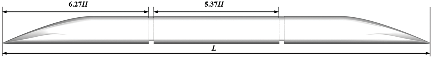
Figure 1: Numerical model of a maglev train

The computational domain is shown in Fig. 2. It has a length of 520 m, width of 80 m, and height of 24 m. The head noses of the two trains are 100 m apart at the initial moment. The railway spacing is 5 m, by default. For the purpose of simulating the relative motion between the trains, the sliding mesh technique is used. The entire flow is divided into a motion zone and a fixed zone. The motion zone includes the train and the grid around it. The fixed zone is the remaining external flow field. The motion zone and fixed zone transmit the grid information through the interface. The flow field partition diagram is shown in Fig. 3.

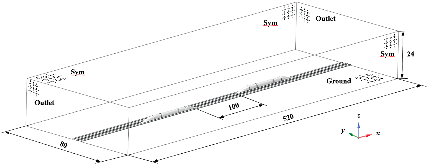
Figure 2: Model and dimensions of the computational domain (m)

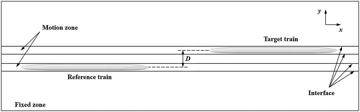
Figure 3: Zones of the flow field

The boundary condition settings are as follows: Pressure outlet is set to the front and rear boundaries of the external flow field. The side and top surfaces are set as symmetry. The interfaces between the motion zone and the fixed zone are set as interface conditions. The surfaces of the ground and the train in the fixed zone are simulated by the standard wall function, using non-slip wall conditions. The motion zone is set as the train running speed, which is 600 km/h. The ground and the rail base in the motion zone are set as moving wall.

2.3 Monitoring Points

A total of 25 monitoring points are arranged on the head car, middle car and tail car, of which four are arranged on the driver’s cab side-windows of both the head and tail cars. Fig. 4 shows the monitoring points. Points H1~H7, M1~M7, and T1~T7 are the body monitoring points. Monitoring points 2~4 are arranged on the train crossing side. Monitoring points 2, 3, 5, and 6 are arranged on the other side. The monitoring points of the driver’s cab side-windows are named WH1, WH2, WT1, and WT2, with points WH1 and WT1 located on the crossing side. When two identical trains meet at the same speed, their aerodynamic characteristics are exactly the same, so the following analysis is carried out on the target train.

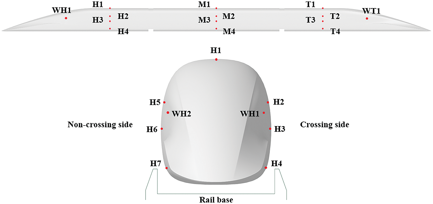
Figure 4: Monitoring points arrangement

2.4 Grid Independence Test

Fig. 5 shows the grid types of the whole flow field, which are all unstructured tetrahedral grids. For the purposes of improving mesh quality and ensuring calculation accuracy, a grid independence test is carried out. By changing the basic size of the flow grid, three sets of grids, being coarse, medium, and fine, were generated. The numbers of the three sets of grids were 35.81 million, 40.24 million, and 44.76 million, respectively. Fig. 6 shows the pressure time history curve at a certain measuring point of the head car, for different meshes. The surface pressure change under different grid numbers is consistent, while the peak value is different. The relative error of the maximum positive peak between the medium grid and the coarse grid is 1.16 %. For the medium grid and the fine grid, the relative error is 0.43%. It can be seen that with the increase in grid number, the calculation error gradually decreases. Considering accuracy and the cost of calculation, the medium grid was selected for subsequent calculation.

Figure 5: Numerical mesh

Figure 6: Time histories of pressure at a certain monitoring point of the head car for different meshes

2.5 Numerical Validation

In order to verify the reliability of the numerical simulation used in this paper, a three-car marshaling train model similar to that used by Wang et al. [21] is adopted. The train model is shown in Fig. 7. The total length of the train is 81.025 m, and the scale ratio is 1:20. Fig. 8 shows the comparison in pressure between the numerical simulation and moving rig test at a certain measuring point on the head car. The pressure variation is essentially consistent. The error of the pressure amplitude between the numerical simulation and test is less than 10%. Therefore, the numerical method used in this study is reliable and can be used to study the aerodynamic characteristics of HSMTs passing each other.

Figure 7: Train model adapted for numerical validation

Figure 8: Comparison between the numerical simulation and the moving rig test, at a certain measuring point of the head car

3  Results

The calculation results are analyzed, mainly focusing on the aerodynamic load of the train, the pressure wave, and the pressure of the flow field.

3.1 Aerodynamic Load

Fig. 9 shows the variation of side force Fs and rolling moment Mx, of the three cars when maglev trains meet at 600 km/h, with a railway spacing of 5 m. The moment center is taken to be the centroid position of the car. The variation of side force and rolling moment of each car have similar patterns, both having two fluctuation changes. This fluctuation is caused by the alternation between positive and negative pressure on the crossing side surfaces of the two trains. It can be seen from Fig. 9 that the Fs fluctuations of the three cars follow a consistent pattern, albeit with different amplitudes. Compared with the head car and the tail car, the rolling moment of the middle car is the smallest, and the fluctuation is not obvious. Therefore, the Fs and Mx of the head car are chosen to study the influence of railway spacing on the aerodynamic characteristics of trains.

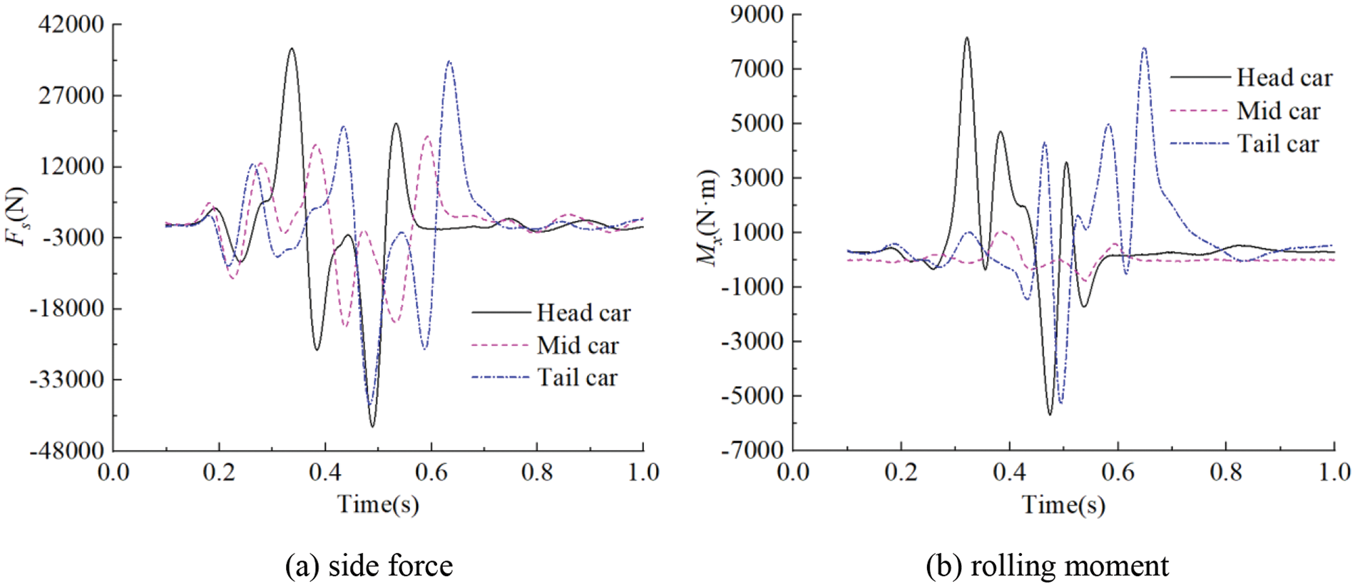
Figure 9: Time histories of side force and rolling moment of three cars

The variation of the Fs and Mx of the head car when maglev trains meet at 600 km/h with different railway spacing (5~5.6 m, with intervals of 0.2 m), are shown in Fig. 10. It can be seen that the Fs and Mx of the head car decrease with the increase in railway spacing. In the period of 0.41~0.43 s, the changes in side force and rolling moment fluctuate unevenly. This occurs because at this moment, the first windshield of the reference train, which is smaller than the car body in terms of cross-section, passes the head car of the target train. This sudden change in cross-sectional area causes the fluctuation.

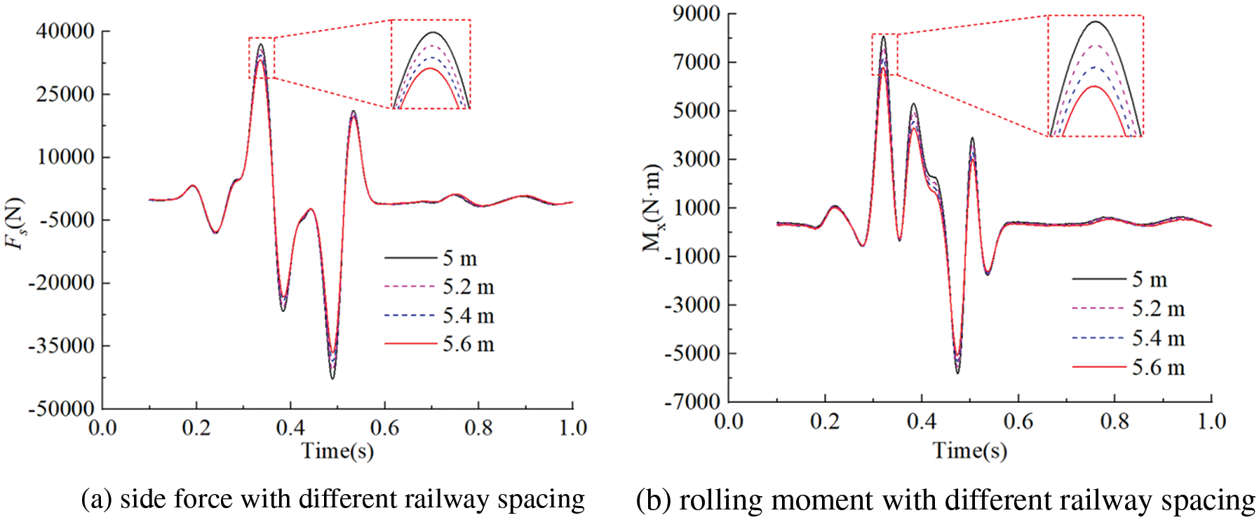
Figure 10: Time histories of side force and rolling moment of head car with different railway spacing

Table 1 shows the Fs and Mx of the head car. The Fs of the vehicle can be calculated by Eq. (2), in which the side force coefficient Cs is unknown. Considering the negative exponential relationship between the pressure wave and the railway spacing [24], the relationship between the side force coefficient and the railway spacing can be fitted by Eq. (3).

Fs=12ρv2CsAs(2)

Cs=aD−b (3)

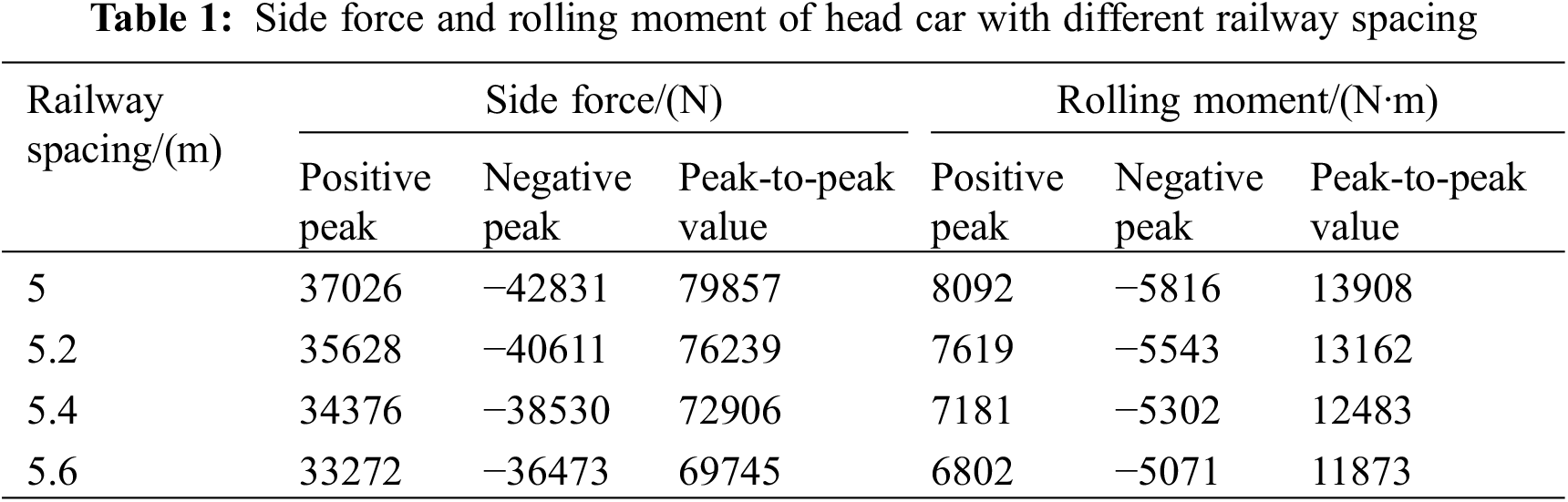
where Fs is the side force, ρ is the air density (1.225 kg/m3), As is the cross-sectional area of the train (8.4 m2), v is the train running speed (166.67 m/s), Cs is the side force coefficient, D is railway spacing, a and b are fitting coefficients.

The peak-to-peak values of the side force with different railway spacing is fitted by:

Fs=1.9058ρv2AsD−1.1929,R2=0.9999,(4)

The relationship between the rolling moment and the railway spacing is similar to the side force. The peak-to-peak value of the rolling moment with the railway spacing is fitted by:

Mx=0.1441ρv2AsdhD−1.3973, R2=1.0(5)

where Mx is the rolling moment, dh=4AsPe is hydraulic diameter (3.2 m), where Pe is the perimeter of the cross-section (10.5 m).

3.2 Surface Pressure

The surface pressure on the crossing side of the target train with a meeting speed of 400 km/h, is shown in Fig. 11. Before the maglev trains meet, a large positive pressure forms on the nose tip of the head car and, due to the accelerating effect of airflow, there is mainly a negative pressure on both sides of the vehicle body. Fig. 11 shows that when the target train is about to reach the nose tip of the reference train, the initial compression wave is formed, and the positive pressure on the head car increases significantly. At the initial moment, most of the vehicle surface on the crossing side experiences negative pressure. When a certain point within the negative pressure area meets the nose tip of the reference train, there will be a large positive pressure area on the target train. As the train meeting continues, this point meets the negative pressure area of the reference train. The positive pressure at this point decreases and changes back to negative pressure. Therefore, an alternating pressure fluctuation between positive and negative will be formed at this point. When the maglev trains are passing each other, the pressure of the target train on the crossing side is affected by the reference train, forming an alternating pressure fluctuation between positive and negative.

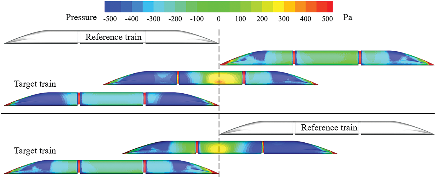
Figure 11: Surface pressure on the crossing side of the target train at 400 km/h

Fig. 12 shows the monitoring points’ pressure values of target train with a railway spacing of 5 m. As shown in Fig. 12, when the train nose of the reference train passes the monitoring points on the target train, a positive pressure peak will be generated first. Then, as the negative pressure area of the reference train passes, the pressure of the monitoring point will decrease sharply and produce a negative pressure peak, that is, a ‘head wave’. When the streamlined part of the tail car of the reference train, which experiences significant negative pressure, passes the monitoring point, a negative pressure peak will be generated first. Then the tail car nose passes, and the pressure will rise sharply to another positive pressure peak, that is the ‘tail wave’. It can be seen in Fig. 12a that the pressure changes of the monitoring points at the same sections of the train have similar tendencies, although the pressure amplitudes are quite different. The pressure wave amplitudes of monitoring points on the crossing side are much larger than those of the non-crossing side. The closer the monitoring point is to the other train, the larger the pressure wave amplitude is, and the pressure wave amplitude of monitoring point 3 is the largest. This phenomenon occurs because both sides of the train are curved, with monitoring point 3 being located at the point of greatest arc curvature, thus having the shortest distance between the two trains on this horizontal plane. Fig. 12b shows the pressure change of points H3, M3, and T3, among which the pressure wave amplitude of the head car is the largest.

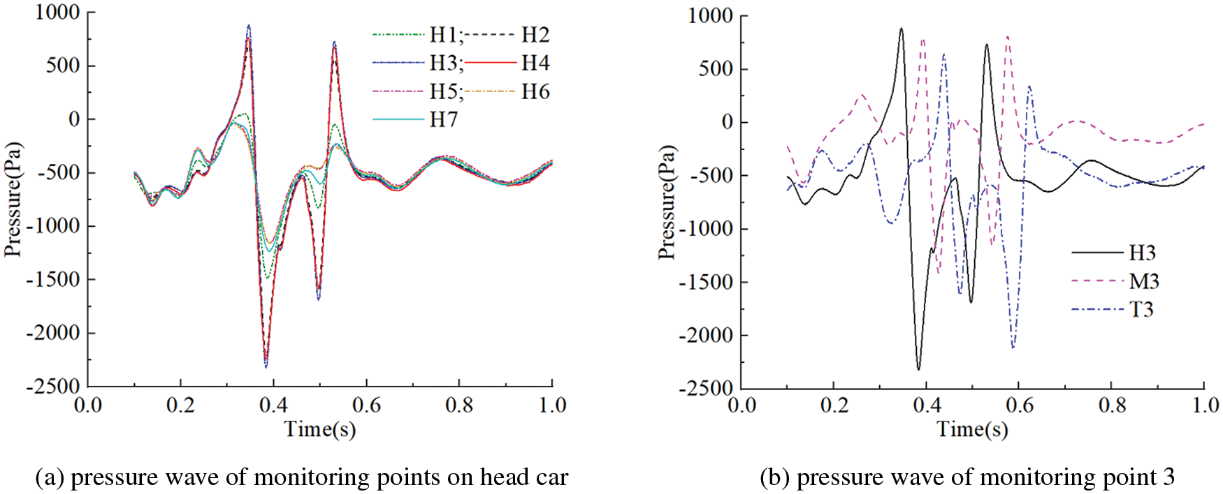
Figure 12: Time histories of pressure of monitoring points at 600 km/h

Fig. 13 gives the pressure changes at monitoring point M3, which is the point of maximum pressure on the middle car when maglev trains meet at different running speeds (400~600 km/h, with intervals of 50 km/h), with a railway spacing of 5 m. As shown, the pressure fluctuations of monitoring point M3 are consistent. With increases in train running speed, the pressure wave amplitudes at the monitoring points on the vehicle surface increase significantly.

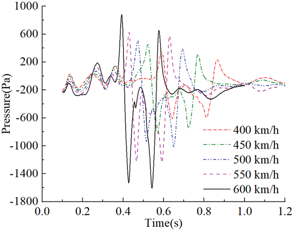
Figure 13: Time histories of pressure of monitoring point M3 at different speed

Table 2 shows the pressure wave peak of the head and tail waves at monitoring point M3, at different running speeds. As given in Table 2, when trains meet at high speed, the positive peak values Pp, negative peak values Pn, and peak-to-peak values ΔP generated by the head wave are significantly larger than those of the tail wave. Therefore, when trains pass each other, the pressure wave generated by the head car has a greater impact than that of the tail car. The ΔP values of the vehicle surface pressure wave are approximately linear with the square of the train running speed v. The peak-to-peak values of head wave and tail wave with different train running speed are fitted by:

ΔPhM=0.6637ρv2,R2=0.9645(6)

ΔPtM=0.6225ρv2,R2=0.9578(7)

where ΔPhM are the ΔP values of the head wave at monitoring point M3, ΔPtM are the ΔP values of the tail wave at monitoring point M3.

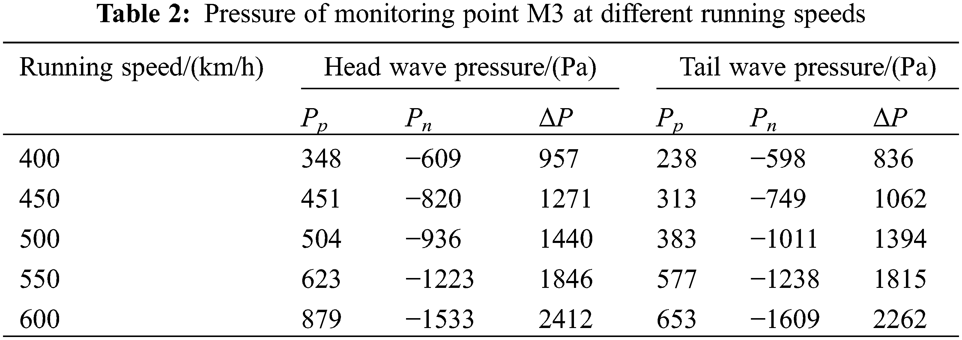
Fig. 14 shows the pressure change of point WH1 at the side-window of the driver’s cab of the head car. From Fig. 14, it can be seen that when maglev trains meet with different railway spacing, the pressure wave changes of point WH1 are consistent.

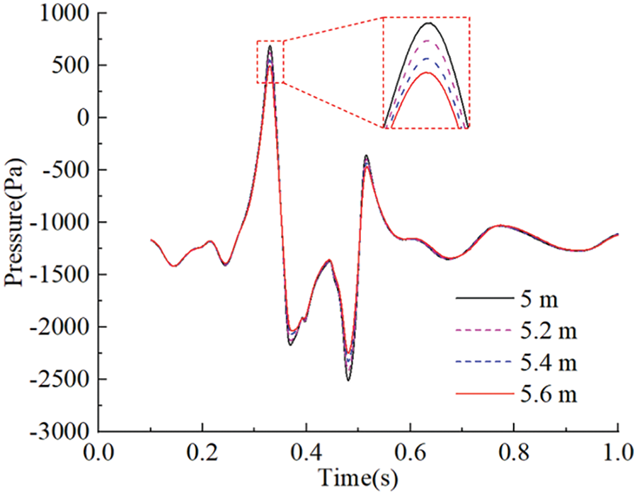
Figure 14: Time histories of pressure of monitoring point WH1 with different railway spacing

Table 3 gives the positive wave peak, negative wave peak, and peak-to-peak values of the head, and tail wave at monitoring point WH1. With increases in the railway spacing, the pressure wave amplitude of monitoring point WH1 gradually decreases. The pressure wave of monitoring point WH1 shows a negative exponential relationship with the railway spacing. Eqs. (8) and (9) can be obtained, by fitting the peak-to-peak values of the head wave and tail wave with different railway spacing.

ΔPhW=0.4923ρv2D−1.0977,R2=0.9962(8)

ΔPtW=0.9126ρv2D−1.6585,R2=1.0(9)

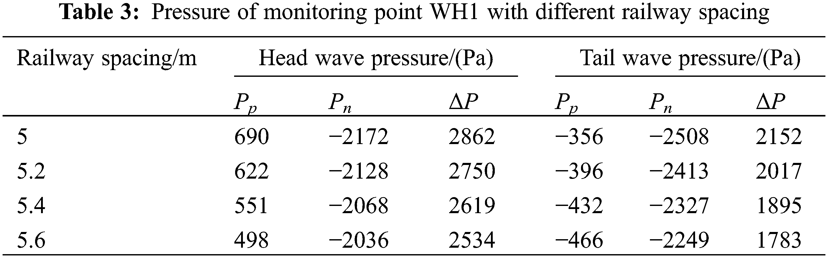
where ΔPhW are the ΔP values of the head wave at monitoring point WH1, and ΔPtW are the ΔP values of the tail wave at monitoring point WH1.

3.3 Flow Field

To explore how maglev trains affect each other’s flow field when they are meeting, three monitoring lines, T, M, and R, are positioned in section P, which is 30 m away from the head nose of the target train. 21 points are set from top to bottom on these monitoring lines, to monitor the pressure changes. The position of section P and the monitoring points are shown in Fig. 15.

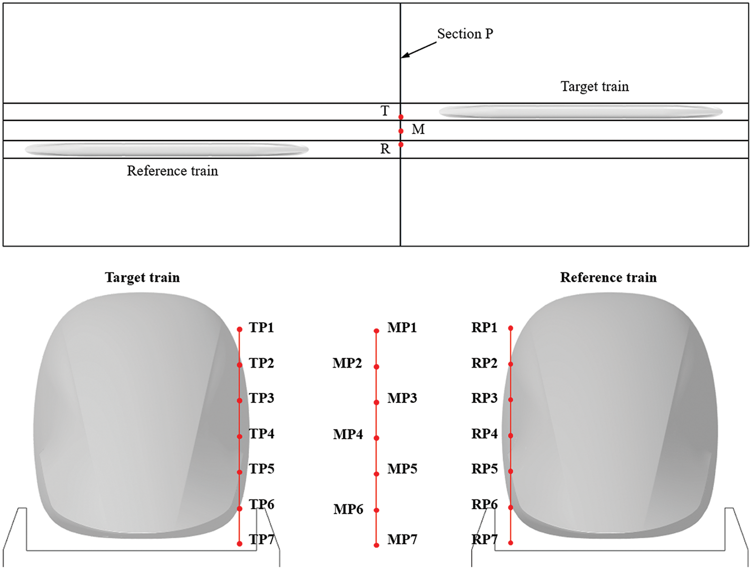
Figure 15: Position of section P and the monitoring points

Fig. 16a shows the pressure at the monitoring points of line M. When the target train reaches section P at 0.18 s and the reference train reaches it at 0.42 s, the pressure change is similar to the head wave. The tail car of the target train passes through the section at about 0.5 s, forming a pressure change similar to the tail wave. At this time, the large negative pressure peak values Pn are caused by the head wave negative pressure of the reference train plus the tail wave negative pressure of the target train. Taking the negative pressure peak as the center of symmetry, the influence of the target train and the reference train on the pressure of the M-line monitoring point are approximately symmetrical. The pressure history at the M-line monitoring point shows that the flow field pressure on the crossing side of the train will experience the combined influence of both trains.

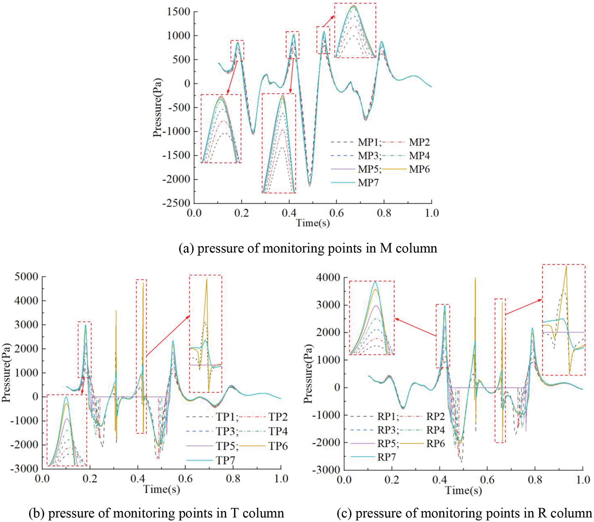
Figure 16: Time histories of pressure of monitoring points in section P

According to Fig. 16b,c, the pressure peak value of the T column is larger than that of the R column when the target train passes, while the R column has a larger pressure wave peak when the reference train passes. Monitoring points 2–5 of the T and R columns are located inside the vehicle when the trains pass, so there is no pressure data at this moment. At 0.31 and 0.42 s in Fig. 16b, and 0.55 and 0.66 s in Fig. 16c, pressure fluctuations occur. The windshield passes through section P at these moments, and the sudden change of cross-section leads to the pressure fluctuations. The surface pressure of the windshield has a large positive value as shown in Fig. 11, which leads to the large positive pressure peak. For TP6, the second windshield of the target train passes through section P at about 0.42 s, and the head nose of the reference train also reaches this position. They significantly increase the positive pressure in combination, and give TP6 a larger positive pressure peak. For RP6, the first windshield of the reference train and the head nose of the target train pass through section P at 0.55 s. They also cause RP6 to have a larger positive pressure peak.

Fig. 17 shows the pressure contour in the horizontal plane of monitoring point RP6 at 0.55 s. RP6 is located in the black dotted box in Fig. 17. An obvious positive pressure zone can be seen between the windshield of the reference train and the rail base inner wall. At the same time, the positive pressure of the target train’s tail nose also reaches section P, resulting in a large positive pressure peak at 0.55 s in Fig. 16c.

Figure 17: Pressure contours in the horizontal plane of monitoring point RP6 at 0.55 s

Fig. 18 demonstrates the pressure change of MP4 in section P when the trains meet at 600 km/h with different railway spacing. It can be seen that the pressure variation pattern of MP4 in section P is consistent. Taking the maximum negative pressure peak near 0.48 s as an example, with an increase of railway spacing, the peak values of the maximum negative pressure magnitudes are 2534, 2382, 2253, and 2139 Pa, respectively. The pressure peak values of flow field monitoring points also exhibit a negative exponential relationship with railway spacing. The fitting equation of the absolute value of the maximum negative pressure peak value with different railway spacing is as follows:

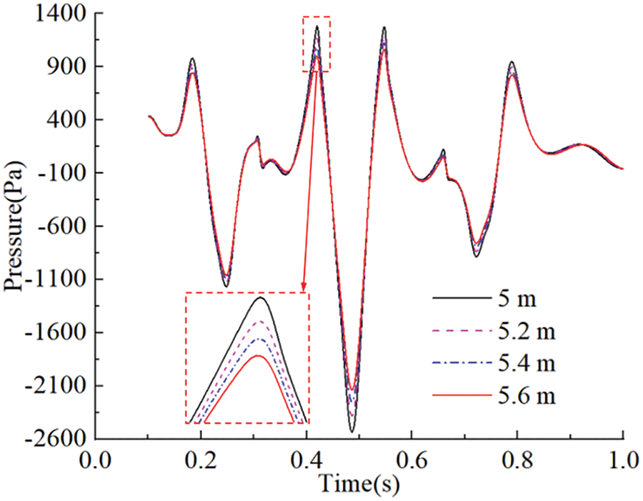
Figure 18: Time histories of pressure of monitoring point MP4 with different railway spacing

Pmax=0.8279ρv2D−1.4973,R2=0.9995(10)

where Pmax is the peak value of the maximum negative pressure magnitude at flow field monitoring point MP4.

4  Conclusion

(1) The variation of vehicle surface pressure when trains pass each other are similar, and the pressure wave amplitude shows considerable differences between various positions. The pressure wave amplitudes at the monitoring points on the vehicle body on the crossing side, are much larger than those of the monitoring points on the non-crossing side.

(2) When high-speed maglev trains meet at 600 km/h with varied railway spacing (5~5.6 m, with intervals of 0.2 m), the vehicle surface pressure variation and the variation of side force and rolling moment are consistent. They all have a negative exponential relationship with railway spacing. As the railway spacing increases from 5 to 5.6 m, the amplitude of the head car’s side force and rolling moment, the vehicle surface pressure amplitude of the head wave and the tail wave, are reduced by 12.7%, 14.6%, 11.5%, and 17.1%, respectively.

(3) At present, although a train model, which has moving rig test data, was adopted to verify the reliability of the numerical simulation method used in this paper, the train model adopted in this paper still lacks moving rig test data or full-scale test data. In addition, the present paper only discusses the aerodynamic characteristics of maglev trains passing each other in open air. However, HSMTs pass each other in multiple situations and settings, including crosswinds, bridges, tunnels, etc., which will be studied in future work.

Acknowledgement: None.

Funding Statement: The research in this paper was supported by the National Natural Science Foundation of China (12372049), Fundamental Research Funds for the Central Universities (2682023ZTPY036), and Research and Development Project of JDD For HTS Maglev Transportation System (JDDKYCF2024002).

Author Contributions: The authors confirm contribution to the paper as follows: study conception and design: Tian Li, Yan Li; data collection: Bailong Sun, Deng Qin; analysis and interpretation of results: Bailong Sun, Tian Li, Deng Qin; draft manuscript preparation: Bailong Sun. All authors reviewed the results and approved the final version of the manuscript.

Availability of Data and Materials: The data presented in this study is available from the corresponding author, upon reasonable request. The data is not publicly available due to privacy.

Ethics Approval: Not applicable.

Conflicts of Interest: The authors declare no conflicts of interest to report regarding the present study.

References

1. Rasulov M, Masharipov M, Bozorov R. Research on the aerodynamics of high-speed trains. Universum: Techn Sci. 2022;6(99):30–5. doi:10.32743/UniTech.2022.99.6.13827. [Google Scholar] [CrossRef]

2. Hyung-Woo L, Ki-Chan K, Ju L. Review of maglev train technologies. IEEE Trans Magn. 2006;42(7):1917–25. doi:10.1109/TMAG.2006.875842. [Google Scholar] [CrossRef]

3. Baker CJ. The flow around high speed trains. J Wind Eng Ind Aerodynamics. 2010;98(6):277–98. doi:10.1016/j.jweia.2009.11.002. [Google Scholar] [CrossRef]

4. Ahmad Imam K. Impact of velocity and wind direction to drag force of commercial train locomotive. J Mech Eng Mechatron. 2022;7(1):2527–6212. doi:10.33021/jmem.v7i1.3390. [Google Scholar] [CrossRef]

5. Muñoz-Paniagua J, García J. Aerodynamic drag optimization of a high-speed train. J Wind Eng Ind Aerodynamics. 2020;204(6):104215. doi:10.1016/j.jweia.2020.104215. [Google Scholar] [CrossRef]

6. Fujii K, Ogawa T. Aerodynamics of high speed trains passing by each other. Comput Fluids. 1995;24(8):897–908. doi:10.1016/0045-7930(95)00024-7. [Google Scholar] [CrossRef]

7. Diedrichs B, Krajnović S, Berg M. On the aerodynamics of car body vibrations of high-speed trains cruising inside tunnels. Eng Appl Comput Fluid Mech. 2008;2(1):51–75. doi:10.1080/19942060.2008.11015211. [Google Scholar] [CrossRef]

8. Raghunathan RS, Kim HD, Setoguchi T. Aerodynamics of high-speed railway train. Prog Aerosp Sci. 2002;38(6):469–514. doi:10.1016/S0376-0421(02)00029-5. [Google Scholar] [CrossRef]

9. Lu Y, Wang T, Yang M, Zhang L, Shi F, Zhu Y, et al. Mitigation of the pressure fluctuation arising from high-speed train intersection in tunnels using enlarged tunnel ends. Tunnelling Undergr Space Technol. 2022;128(2):104634–45. doi:10.1016/j.tust.2022.104634. [Google Scholar] [CrossRef]

10. Hwang J, Lee D-H. Unsteady aerodynamic loads on high speed trains passing by each other. KSME Int J. 2000;14(8):867–78. doi:10.1007/BF03184475. [Google Scholar] [CrossRef]

11. Zhao Y, Zhang J, Li T, Zhang W. Aerodynamic performances and vehicle dynamic response of high-speed trains passing each other. J Mod Transp. 2012;20(1):36–43. doi:10.1007/BF03325775. [Google Scholar] [CrossRef]

12. Zhang Q, Cai X, Wang T, Zhang Y, Wang C. Aerodynamic performance and dynamic response of high-speed trains passing by each other on cable-stayed bridge under crosswind. J Wind Eng Ind Aerodynamics. 2024;247(6–7):105701–17. doi:10.1016/j.jweia.2024.105701. [Google Scholar] [CrossRef]

13. MacNeill RA, Holmes S, Lee HS. Measurement of the aerodynamic pressures produced by passing trains. In: ASME/IEEE Joint Railroad Conference, 2002; Wanshington, DC, USA: IEEE; p. 57–64. doi:10.1109/rrcon.2002.1000094. [Google Scholar] [CrossRef]

14. Mancini G, Malfatti A. Full scale measurements on high speed train Etr 500 passing in open air and in tunnels of Italian high speed line. In: TRANSAERO—A European initiative on transient aerodynamics for railway system optimisation. 2002. p. 101–22. doi:10.1007/978-3-540-45854-8_9. [Google Scholar] [CrossRef]

15. Bell JR, Burton D, Thompson M, Herbst A, Sheridan J. Wind tunnel analysis of the slipstream and wake of a high-speed train. J Wind Eng Ind Aerodynamics. 2014;134(4):122–38. doi:10.1016/j.jweia.2014.09.004. [Google Scholar] [CrossRef]

16. Johnson T, Dalley S. 1/25 scale moving model tests for the transaero project. In: TRANSAERO—A European initiative on transient aerodynamics for railway system optimisation. 2002. p. 123–35. doi:10.1007/978-3-540-45854-8_10. [Google Scholar] [CrossRef]

17. Saito S, Iida M, Kajiyama H. Numerical simulation of 1-d unsteady compressible flow in railway tunnels. J Environ Eng. 2011;6(4):723–38. doi:10.1299/jee.6.723. [Google Scholar] [CrossRef]

18. Yamamoto K, Kozuma Y, Tagawa N, Hosaka S, Tsunoda H. Improving maglev vehicle characteristics for the Yamanashi test line. Q Rep RTRI. 2004;45(1):7–12. doi:10.2219/rtriqr.45.7. [Google Scholar] [CrossRef]

19. Huang S, Li Z, Yang M. Aerodynamics of high-speed maglev trains passing each other in open air. J Wind Eng Ind Aerodynamics. 2019;188(2):151–60. doi:10.1016/j.jweia.2019.02.025. [Google Scholar] [CrossRef]

20. Li X, Krajnovic S, Zhou D. Numerical study of the unsteady aerodynamic performance of two maglev trains passing each other in open air using different turbulence models. Appl Sci. 2021;11(24):11894–913. doi:10.3390/app112411894. [Google Scholar] [CrossRef]

21. Wang F, Zhang L, Yang MZ, Yin XF. Effect of line space on aerodynamic performance of two high-speed maglev trains passing by each other at the speed of 600 km/h in open air. Acta Aerodynamica Sinica. 2023;41(4):31–40 (In Chinese). doi:10.7638/kqdlxxb-2021.0122. [Google Scholar] [CrossRef]

22. Li T, Qin D, Zhou N, Zhang W. Step-by-step numerical prediction of aerodynamic noise generated by high speed trains. Chin J Mech Eng. 2022;35(1):28. doi:10.1186/s10033-022-00705-4. [Google Scholar] [CrossRef]

23. Qin D, Du X, Li T, Zhang JY. Numerical study on reduction in aerodynamic drag and noise of high-speed pantograph. Comput Model Eng Sci. 2024;139(2):2155–73. doi:10.32604/cmes.2023.044460. [Google Scholar] [CrossRef]

24. Tian HQ. Research and applications of air pressure pulse from trains passing each other. J Railway Sci Eng. 2004;1(1):83–9. doi:10.19713/j.cnki.43-1423/u.2004.01.015. [Google Scholar] [CrossRef]