Molecular Dynamics Simulation of Bubble Arrangement and Cavitation Number Influence on Collapse Characteristics

1  Introduction

With the development of the precision of electronic units, microfluidic electronic units with diverse structures have emerged, drawing significant attention to the issue of sub-microscopic cavitation. Cavitation is visually represented by the formation of bubbles, which typically occur in clusters rather than as isolated entities. The bubbles will interact, interfere, and intercoupling [1,2]. Upon collapse, the bubbles release energy, creating extreme conditions such as elevated temperatures [3], high pressures [4], and the formation of microjets [5]. These extreme conditions can cause damage to electronic components and fluid-mechanical devices. However, due to experimental limitations, research on the collapse mechanisms of multiple bubbles remains insufficient, emphasizing the need for further investigation into this process.

Molecular dynamics simulation is a micro- and nanoscale method used to reveal the characteristics of bubble collapse by analyzing molecular motion. There are many factors that affect bubble collapse, such as bubble radius [6,7], temperature [8], fluid medium [9], the gas contained within the bubble [10], and shock wave velocity [11]. Mahmud et al. [12] investigated the pressure required for the growth of nanobubbles in water and gels, concluding that the viscosity of the medium determines the bubble collapse time. He et al. [13] and Nan et al. [14] studied the motion of a single bubble during its ascent in a magnetic fluid, finding that the bubble shape transforms from an oblate ellipse to an oblate elliptical cap in the magnetic fluid. Dockar et al. [15] studied the effects of contact angle on bubble collapse, finding that the depression depth of surface bubble collapse depends on the contact angle rather than bubble size.

In addition, numerous scholars have investigated the physical properties of bubbles collapse. Adhikari et al. [16−18] explored the mechanisms underlying soft material damage caused by the collapse of nanobubbles due to shock waves, and found that the size of lipid membrane perforations depends on the shock wave velocity and its duration. Wu et al. [19] studied the effects of bubble position, shock wave intensity, and bubble radius on the structural evolution of neural networks. Nomura et al. [20] investigated the role of shock-induced bubble collapse on the lipid bilayers and reported that the formation of nano jet significantly deformed and thinned the lipid bilayers. Hong et al. [21] and Vedadi et al. [22] investigated molecular mechanisms of hydrocarbon cracking in heavy crude oil promoted by nanobubble collapse due to ultrasound-originated shock wave, and found that high-energy nano-jets are formed during the collapse of nanobubbles.

While extensive research exists on single-bubble dynamics, further systematic studies on the collapse of multi-bubble systems are required. Existing investigations primarily focus on parameters such as impact velocity, bubble radius, and ionic concentration. And the complex interactions of multiple bubbles significantly complicate the dynamics. This paper aims to bridge this gap by establishing a multiple-bubble model that considers various bubble numbers and arrangements.

By employing a combination of molecular dynamics simulation and coarse-grained force field, this paper examines the kinetic behavior of multi-bubble systems under shock wave. The study analyzes bubble collapse morphology, local density distributions, and local pressure distributions, summarizing the influence of bubble number and arrangement on the collapse process. Ultimately, this work aims to clarify the interactions of bubbles in multi-bubble systems, providing valuable insights to enhance the reliability and durability of microfluidic electronic devices subjected to cavitation and shock wave.

2  Simulation Methods

2.1 Model Building

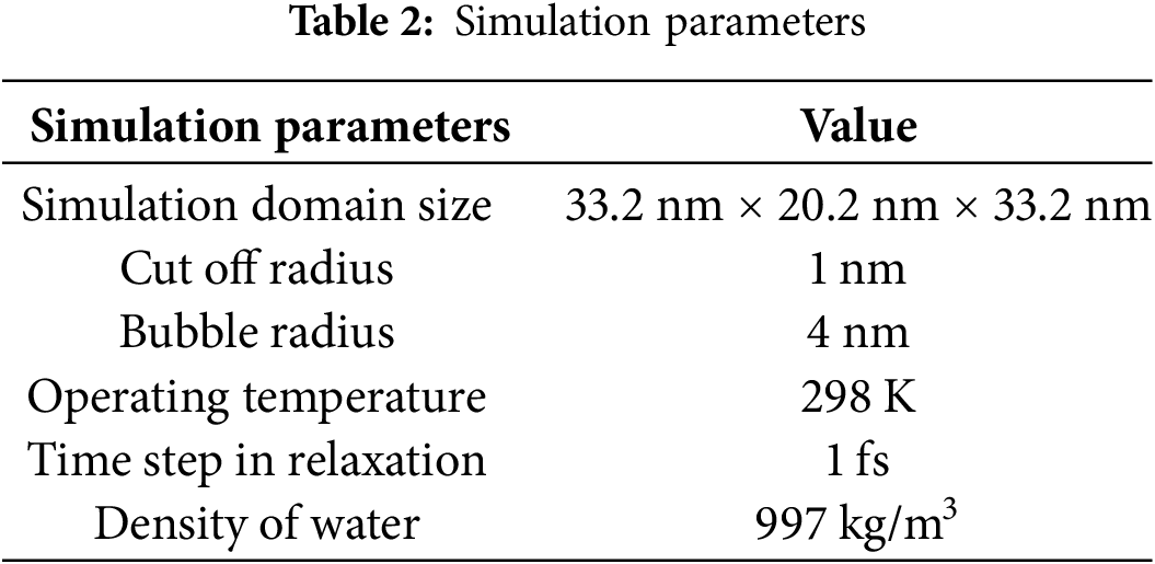
The computational domain in the model measures 33.2 nm × 20.2 nm × 33.2 nm and contains approximately 600,000 water molecules. A schematic diagram of the water molecule and bubble calculation model is presented in Fig. 1. In this study, Materials Studio software is employed to establish the initial coordinates of water molecules [23]. Additionally, a combination of Packmol software and Visual Molecular Dynamics (VMD) software is utilized to create 10 geometrical models, each featuring a different number of bubbles [24,25]. The illustrations of models are shown in Table 1. In addition, the bubbles in this study do not contain gas. This decision is based on the fact that bubbles without gas exhibit significantly higher system pressure compared to gas-containing bubbles [26]. Furthermore, bubbles without gas release greater transient energy during collapse, resulting in a more pronounced impact on the surrounding environment [27]. Accordingly, this study focuses exclusively on the behavior of gas-free bubbles.

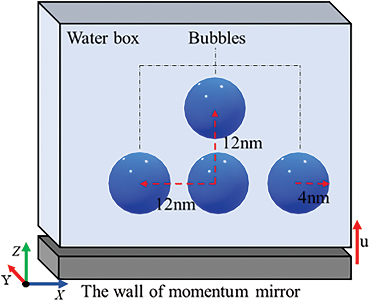
Figure 1: Schematic diagram of calculation model of water molecule and multiple bubbles

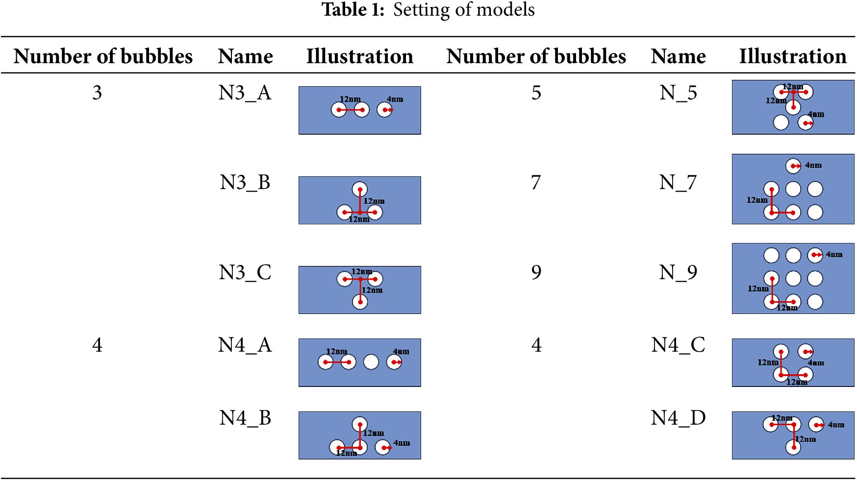
Fig. 1 shows the diagram of the multi-bubble model. In both Fig. 1 and Table 1, the bubble radius is 4 nm, with horizontal and vertical bubble distances both are 12 nm. Shock waves are generated by the method of momentum mirror [28]. And the shock wave is along the Z-axis direction from the bottom to the top with a shock velocity of 1 km/s.

The simulation details presented in Table 1 are categorized into three groups: odd-numbered bubbles (three bubbles), even-numbered bubbles (four bubbles), and odd-multiple bubbles (five, seven, and nine bubbles). The odd-numbered bubbles include three arrangements: N3_A, N3_B, and N3_C. The even-numbered bubbles include four arrangements: N4_A, N4_B, N4_C, and N4_D. The odd-multiple bubbles include three arrangements: N_5, N_7, and N_9. The model and simulation parameter settings are summarized in Table 2.

2.2 Force Field Selection

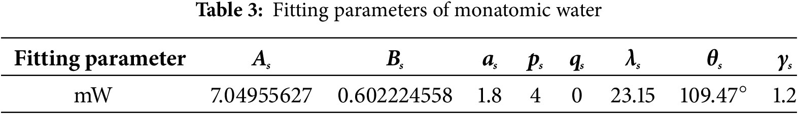
In this study, a coarse-grained force field is employed for the water molecules. The monatomic water (mW) model is used to represent the liquid phase [29]. The interactions in the mW model are described by the Stillinger–Weber (SW) potential [15], as expressed in Eq. (1):

Usw=∑i∑j>iAsεij[Bs(σijrij)ps−(σijrij)qs]×exp⁡(σijrij−asσij)+∑i∑j≠i∑k>jλsεij[cos⁡θjik−cos⁡θs]2×exp⁡(γsσijrij−asσij)exp⁡(γsσikrik−asσik)(1)

In Eq. (1), USW is the total potential energy between the interactions of the atomic/molecular system through the SW potential. The distance between atoms i and j is rij, the distance between i and k is rik, and atoms j and k form an angle θjik with atom i. Coarse-grained particles interactions are all calculated using the Lennard-Jones (LJ) potential [30]:

ULJ=∑i∑j>i4εij[(σijrij)12−(σijrij)6](2)

In Eq. (2), ULJ is the total potential energy of all LJ potential interactions.

2.3 Parameter Setting

The specific material properties in Eq. (1) are obtained by fitting the parameter As, Bs, as, ps, qs, λs, θs, γs as shown in Table 3 [30]. In Eq. (2), the potential parameters ε and σ are the potential trap depth and bond length, respectively, with specific values shown in Table 4.

Before performing molecular dynamics simulations, the model must undergo a relaxation process. This process is essentially a dynamic procedure in which microscopic particles exchange energy within the system until a stable distribution is achieved. Temperature variation is a key parameter for assessing whether the system has reached a steady state during relaxation. In a steady state, the temperature fluctuates around a constant value. As can be seen in Fig. 2, during relaxation, the temperature initially increases, then decreases, and eventually stabilizes at the value prescribed by the program to maintain dynamic equilibrium. Additionally, the system density remains unchanged throughout the process, with a value close to 997 kg/m3.

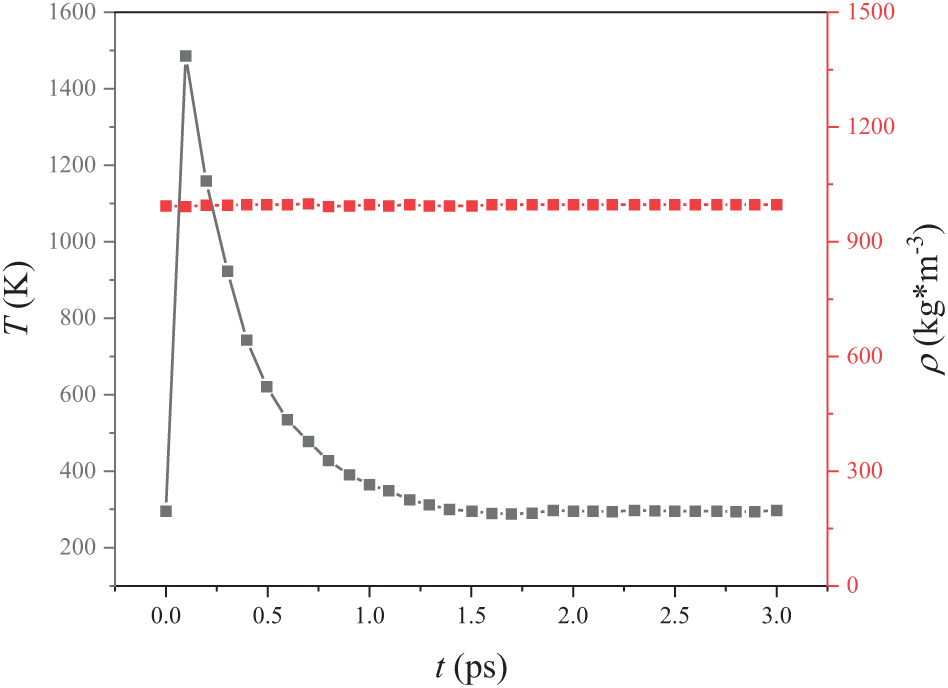
Figure 2: Plot of temperature and density variation with time during the relaxation process

Firstly, the energy of the model is minimized using the steepest descent method. Secondly, the system is equilibrated for 100 ps in canonical ensemble (NVT) at T = 298 K with a timestep of 0.001 ps. Temperature coupling is achieved using the Nose-Hoover method [31]. Thirdly, the system is equilibrated for 30 ps in isothermal-isobaric ensemble (NPT) at a pressure of 1 × 105 Pa, with a timestep of 0.002 ps and a time constant of 0.2 ps. Pressure coupling is achieved using the Parrinello-Rahman method [32] with a time constant of 2 ps.

In the simulation, the cutoff radius is 1 nm. The system’s initial velocity follows the Maxwell–Boltzmann distribution and is randomly generated according to the Maxwell distribution at the corresponding temperature. The Verlet algorithm [33] is employed to numerically solve the Newtonian equations of motion, while the thermal bath coupling method is used for temperature control. Simulation results are output every 100 steps.

3  Results and Discussion

3.1 Analysis of the Evolution Law of Multi-Bubble Collapse Patterns

3.1.1 The Odd-Numbered Bubbles and Their Arrangement on the Collapse Morphology

This section studies the bubble collapse morphology under different arrangements of odd-numbered bubbles. Three specific arrangements are analyzed: N3_A, N3_B and N3_C. In the N3_A arrangement, all three bubbles receive a parallel impact, focusing on the interactions among three symmetrically positioned bubbles. In the N3_B arrangement, only the two lower bubbles receive a parallel impact. In the N3_C arrangement, only the lower single bubble receives a parallel impact.

In this paper, the boundaries of the bubble surface are determined by the simplified R-P equation as well as the condensation and evaporation control equation as follows:

ρ1[RR¨+32(R˙)2]=PV−P∞(3)

∂∂t(αvρv)+∂∂xj(αvρvuj)=Re−Rc(4)

Re=ρvρ1ρmαv(1−αv)3R2(PV−P∞)3ρ1(5)

Rc=ρvρlρmαv(1−αv)3R2(P∞−PV)3ρ1(6)

where ρ1 is the density of liquid; ρν is the density of vapor; R is the bubble radius; R¨ is the second derivative of the bubble radius over time, that is, acceleration; R˙ is the first derivative of the bubble radius over time, that is, velocity; PV is saturated vapor pressure; P∞ is external pressure; αν is the volume fraction of vapor; Re and Rc are the mass transfer rates for bubble evaporation and condensation, respectively.

Under the N3_A arrangement, Fig. 3 shows the slices of the velocity distribution of water molecules, the evolution of the bubble collapse morphology, and the cross-sectional areas A* of the three bubbles. The slices are taken through the center of the three spherical bubbles, each with an initial radius of 4 nm. Initially, the bubble is a regular sphere. At 4.5 ps, the shock wave reaches the bottom of the bubbles. The rightmost bubble collapses completely first at 8 ps. At 8.5 ps, all bubbles collapse completely. As seen in Fig. 3a,b, the bubbles exhibit irregular morphologies during the collapse process. The bubble collapse rate is relatively slow during the early stage (0–4.5 ps) but increases significantly between 5–8 ps. During the initial collapse, the bubble is in a compressed state, and their surface tension can resist a certain external pressure. As a result, the volume of the bubbles changes only slightly in the early stages. As the collapse progresses, the surface tension becomes insufficient to counteract the external pressure, causing the bubble volume to decrease continuously. Microscopically there are intermolecular forces between water molecules, which condense the water molecules and lead to increasingly irregular bubble shapes during the collapse process.

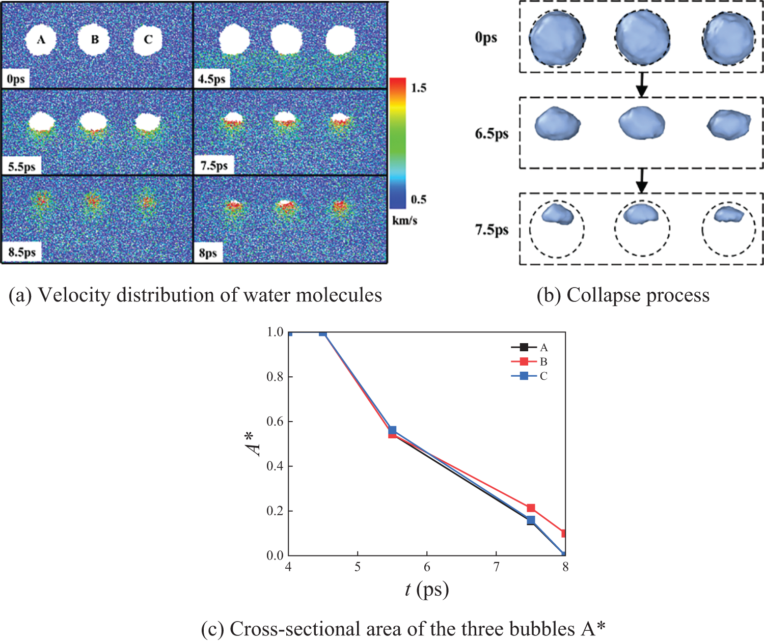
Figure 3: N3_A three-bubble collapse process

From Fig. 3c, it can be observed that, during the initial stage, the cross-sectional areas of the bubbles change at nearly the same rate. However, as the collapse progresses, the cross-sectional areas of the unbounded bubbles on both sides decrease more rapidly. The collapse time of the side bubbles is noticeably shorter than that of the middle bubble. This phenomenon occurs because, during bubble collapse, the surrounding liquid can quickly fill the volume vacated by the collapsing side bubbles. In contrast, the middle bubble is influenced by the presence of the bubbles on either side, preventing the liquid from filling the released volume as efficiently. Consequently, the unbounded bubbles on the sides collapse faster, and their collapse time is shorter than that of the middle bubble.

Fig. 4 shows the evolution of the bubble collapse morphology under the N3_B arrangement, where the initial radius of all three bubbles is 4 nm. In Fig. 4a, it can be observed that the velocity of water molecules below the bubble is significantly higher than that on both sides. Additionally, the two lower bubbles show a slight tendency to move closer to each other. At 3 ps, the shock wave reaches the bottom of the bubbles, and the two lower side bubbles begin collapsing at 7 ps. By 11 ps, all three bubbles have completely collapsed. It can also be seen in Fig. 4b that the two lower side bubbles are subjected to a direct shock wave effect, leading to more pronounced morphological changes. The upper side bubble is subjected to less shock wave effect and is mainly affected by the two lower side bubbles, which have stably morphological changes.

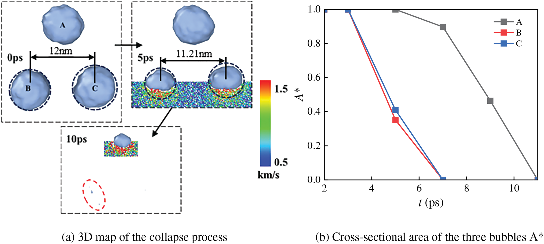
Figure 4: N3_B three-bubble collapse process

Fig. 5 shows the evolution of the bubble collapse morphology under the N3_C arrangement, where the initial radius of all three bubbles is 4 nm. Initially, the bubble interfaces form nearly perfect circles. As time progresses, the shock wave reaches the bottom of the bubbles at 3 ps, and the single lower bubble begins to collapse at 7 ps. By 11 ps, all bubbles have completely collapsed. The water molecule velocity distribution indicates that the velocity on both sides of bubbles is relatively small during the collapse process. From Fig. 5b, it can be observed that, throughout the collapse process, the average collapse speed of the lower bubbles is greater than that of the upper bubble. This suggests that the lower bubbles are directly impacted by the shock wave, resulting in more pronounced morphological changes. The direct influence of the shock wave causes the shapes of the lower bubbles to become more dynamic and complex. The upper bubble is influenced by a combination of the shock wave and the collapsing lower bubbles, leading to a relatively stable collapse process.

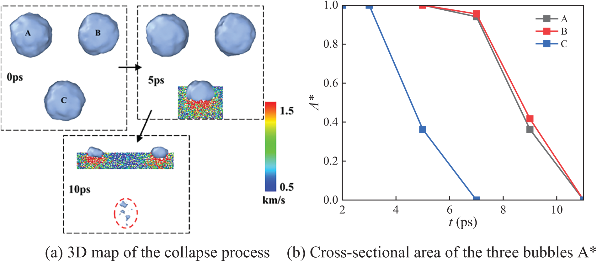
Figure 5: N3_C three-bubble collapse process

In summary, the two unbounded bubbles on both sides collapsed faster than the middle bubble, resulting in a significantly shorter collapse time for the side bubbles compared to the middle one. The upper two bubbles, subjected to the combined effects of the shock wave and the single lower bubble during the collapse process, exhibit a more stable collapse behavior compared to the single upper bubble.

3.1.2 The Even-Numbered Bubbles and Their Arrangement on the Collapse Morphology

This section examines the bubble collapse morphology under different arrangements of even-numbered bubbles. Four specific arrangements are analyzed: N4_A, N4_B, N4_C and N4_D. In the N4_A arrangement, the bubble receives parallel impacts to study the interaction between the four asymmetric bubbles. In contrast, the N4_B, N4_C, and N4_D arrangements investigate bubble interactions under parallel shocks applied to three bubbles, two bubbles, and a single bubble, respectively.

Under the N4_A arrangement, Fig. 6 shows the slices of the water molecule velocity distribution, the evolution of the bubble collapse morphology, and cross-sectional slices through the center of the spheres. The initial radius of the four bubbles is all 4 nm.

Figure 6: N4_A three-bubble collapse process

From Fig. 6, he four bubbles gradually collapsed upon impact, with complete collapse occurring at 8.5 ps. At 7.5 ps, as depicted in Fig. 6a, the water molecules of the rightmost bubble exhibited higher velocity, resulting in more pronounced volume changes, as shown in Fig. 6b. The middle bubbles show relatively little morphological change compared to the outer bubbles during the collapse process. This is attributed to the influence of adjacent bubbles, which decelerates their morphological evolution. This finding highlights the influence of the interactions between the bubbles in the system on evolutionary behavior.

Fig. 7a–c shows the morphological evolution of bubble collapse under the arrangement of N4_B, N4_C, and N4_D, respectively. In collapse process, the bubbles at the lower side collapse first and disappear completely by 10, 10, and 9 ps, respectively. Compared with bubbles on the lower side, the water molecule velocity of the upper side bubble is lower during collapse. On the one hand, it is because the upper-side bubble experiences less influence from the lower-side bubbles. On the other hand, the shock wave’s intensity diminishes as it propagates to the upper-side bubble, leading to a relatively low water molecule velocity.

Figure 7: Four-bubble collapse process

In summary, a comparison of bubble collapse processes under various arrangements indicates that the initial bubble states are essentially spherical. Bubble collapse processes occur more rapidly when directly subjected to a shock wave. Moreover, compared with bubbles on the lower side, the water molecule velocity of the upper side bubble is lower during collapse.

3.1.3 The Odd-Numbered Group Bubbles on the Collapse Morphology

This section examines the bubble collapse morphology under different arrangements of odd-numbered bubbles. Three specific arrangements are analyzed: N_5, N_7, and N_9.

Fig. 8a–c shows the slice diagrams of the velocity distribution of water molecules under the arrangement of N_5, N_7, and N_9, respectively. In Fig. 8a, at 0 ps, the bubble’s interfaces appear essentially circular. At 5 ps, the shock wave propagates to the bottom bubble. By 7.5 ps, the two lower bubbles first collapse. By 9.5 ps, the middle bubble completely collapses. After 11.5 ps, the two bubbles above have also collapsed. In Fig. 8b, at 1 ps, the shock wave reaches the bottom bubble. The lower-side bubbles completely collapse at 6 ps. The middle bubbles completely collapse at 10 ps. After 14 ps, the single upper bubble collapses. The bubbles in N_9 arrangement have the same law of change as the bubbles in N_7 arrangement.

Figure 8: Multi-bubble collapse process

It can be seen from Fig. 8 that during bubbles collapse, the liquid occupying the released volume of the bubble collapsing has a high velocity, which leads to the formation of a micro-jet. And bubbles collapse more rapidly when directly subjected to shock. Moreover, the collapsing bubbles impact adjacent non-collapsed bubbles. Compared with bubbles on the lower side, the water molecule velocity of the upper side bubble is lower during collapse.

3.2 Analysis of the Local Density Distribution during the Multi-Bubble Collapse

3.2.1 The Odd-Numbered Bubbles and Arrangement on the Local Density

In this section, the variation in local density during the shock wave-induced bubble collapse process under three arrangements is analyzed, N3_A, N3_B, and N3_C. The local density is calculated by defining the atomic number density within the volume cell. Specifically, the formula for the local density can be expressed as:

ρlocal=mV(7)

where ρlocal is local density; m is total mass of atoms in the cell; V is the volume, and the cell size is 0.05 nm × 0.05 nm × 0.05 nm.

The computational results are presented in Figs. 9–11, respectively. From Fig. 9a, three low-density regions are observed along the X-direction at positions of 12, 24, and 36 nm. As bubble collapsing, the density at the bubble’s center gradually increases. From Fig. 9b, it can be seen that the initial density increase rates at the centers of the three bubbles are nearly identical. However, as the collapse advances, the density increase rates at centers of the bubbles on the two sides surpass that of the middle bubble, indicating more rapid volume change of the two side bubbles.

Figure 9: N3_A collapse process

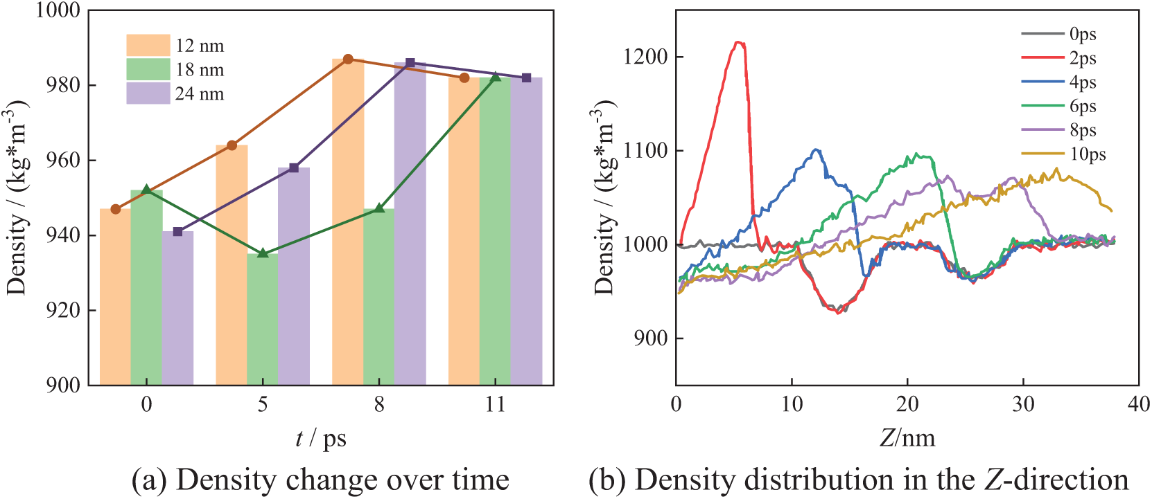
Figure 10: N3_B collapse process

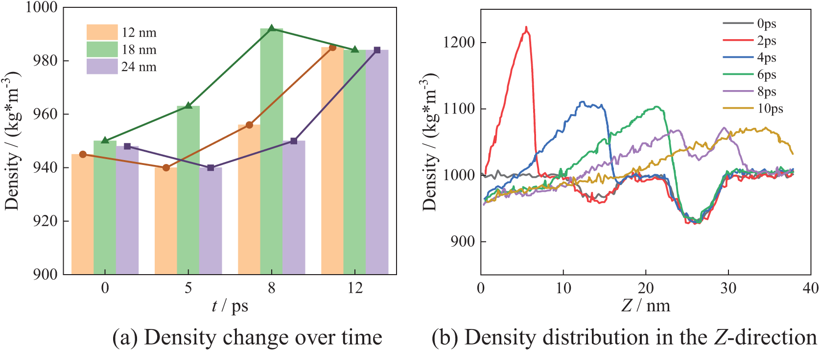
Figure 11: N3_C collapse process

Fig. 9c shows that at 2 ps, the shock wave begins to form, resulting in a local density of up to 1220 kg/m3 in the Z-direction. As bubbles collapsing, the low-density regions gradually shrink. By 10 ps, the maximum density in the Z-direction decreases to 1080 kg/m3, and the density progressively returns to the theoretical density of water after bubbles collapses completely. Moreover, When the bubbles begin to collapse, the density increase instantaneously, and it begins to decrease after a certain distance. This indicates that the energy released by bubbles can prompt the water molecules to aggregate for a short period.

Fig. 10 shows the bubble collapse process in the N3_B arrangement. Similarly, there are regions of low density at the center of bubbles, i.e., 12, 18, and 24 nm.

As shown in Fig. 10a, at X = 12 nm and X = 24 nm, the density gradually increases during the bubble collapse until it reaches the theoretical density of water. At X = 18 nm, the density initially decreases with the bubble collapse and then gradually increases, eventually returning to the theoretical density of water. This phenomenon may occur because 18 nm corresponds to the position of the uppermost bubble, which has not yet begun collapsing when the lower two bubbles initiate their collapse. The influence of the collapsing lower bubbles reduces the local density at the center of the upper bubble. In Fig. 10b, at 2 ps, the density distribution resembles that in Fig. 8b, with a maximum water density of 1210 kg/m3 in the Z-direction. Over time, the bubbles begin to collapse, causing the low-density region to gradually shrink. By 10 ps, the maximum density in the Z-direction decreases to 1080 kg/m3. After bubbles collapse completely, the density gradually returns to the theoretical density of water.

Fig. 11 shows the bubble collapse process in the N3_C arrangement. The position of low-density regions is the same as in the N3_B arrangement.

From Fig. 11a, it can be seen that at X = 12 nm and X = 24 nm, the density decreases initially and then gradually increases as bubbles collapse. And at X = 18 nm, the density gradually increases as bubbles collapse. Ultimately, the density at all three locations reaches the theoretical density of water. This phenomenon may occur because the positions at 12 and 24 nm correspond to the uppermost bubbles, which remain unaffected initially when the lower bubble starts collapsing. The interaction between the collapsing lower bubble and the upper bubbles temporarily reduces the local density at the center of the uppermost bubbles. In Fig. 11b, at 2 ps, the density distribution is similar to Fig. 9b, with a maximum density is 1220 kg/m3 in the Z-direction. As time passes, the bubbles begin to collapse, and the low-density region gradually shrinks. By 10 ps, the maximum density in the Z-direction decreases to 1070 kg/m3. After bubbles collapse completely, the density also gradually returns to the theoretical density of water.

3.2.2 The Even-Numbered Bubbles and Arrangement on the Local Density

In the four-bubble collapse model, when the bubbles are arranged in the N4_A configuration, it is observed that the density distributions along the X and Z directions are consistent with those in the N3_A arrangement, differing only in magnitude. This section focuses on the study of bubble collapse in the N4_B and N4_C.

Fig. 12 shows the bubble collapse process in the N4_B arrangement. The position of low-density regions is the same as in the N3_A arrangement. The Fig. 12b shows the density distribution along the Z-axis direction. The two low-density regions exist near 14 and 26 nm, with the density at 14 nm being higher than that at 26 nm. These low-density regions correspond to the centers of the four bubbles.

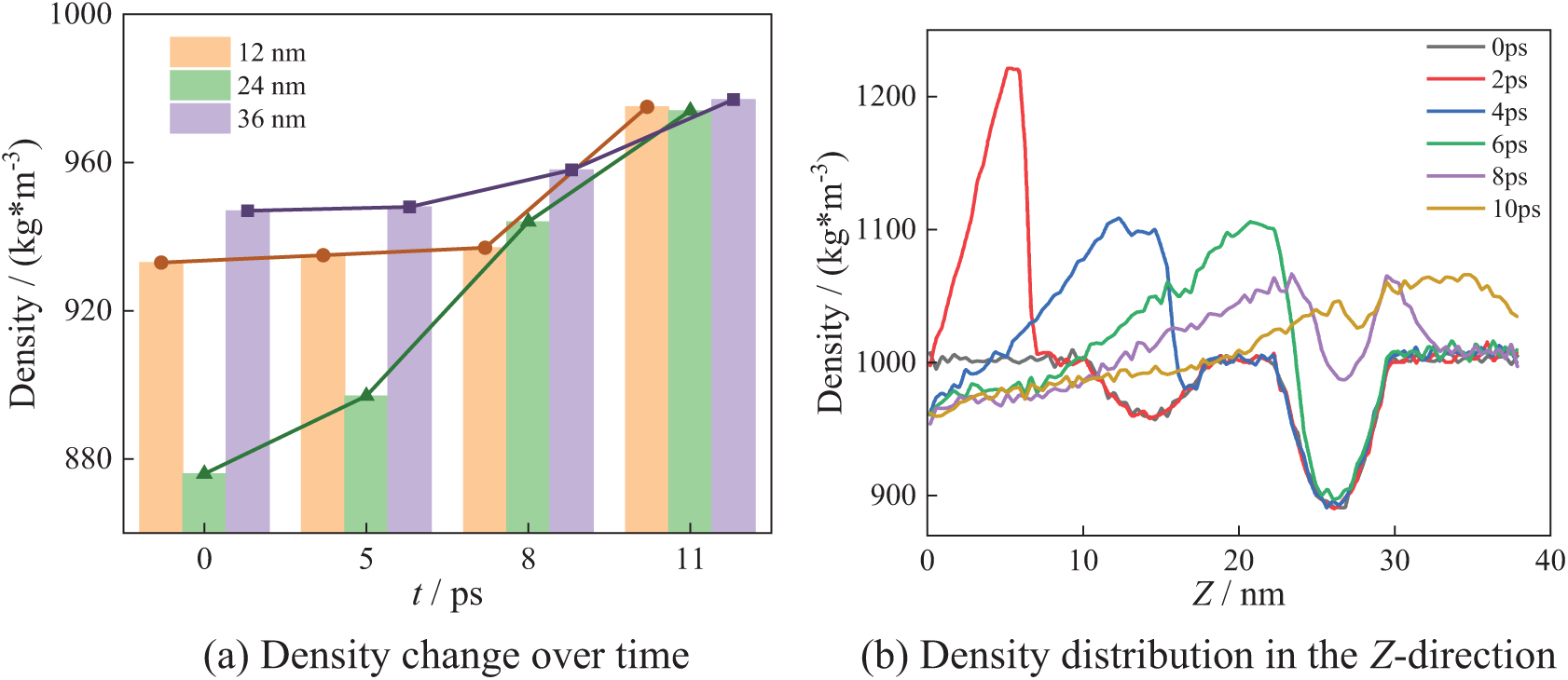
Figure 12: N4_B collapse process

As can be seen from Fig. 12a, at X = 12 nm and X = 36 nm, the density is constant at the beginning of the bubble collapse and then gradually increases. At 24 nm, with bubble collapse, the density increases rapidly. In Fig. 12b, at 2 ps, the density distribution resembles that in Fig. 8b, with a maximum water density of 1220 kg/m3 in the Z-direction. As the bubbles collapse, the low-density region gradually narrows. By 4 ps, he density in the previously low-density region exceeds 1000 kg/m3, indicating that the impact energy released by the bubble collapse caused local water molecule aggregation. At 10 ps, the maximum density decreases to 1070 kg/m3. After bubbles collapse completely, the system density gradually returns to the theoretical density of water.

Fig. 13 shows the bubble collapse process in the N4_B arrangement. Similarly, low-density regions are observed at the centers of the bubbles, i.e., 12 and 24 nm.

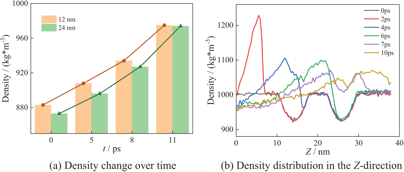
Figure 13: N4_C collapse process

As can be seen from Fig. 13a, at X = 12 nm and X = 24 nm, the density gradually increases during the bubble collapse until it reaches the theoretical density of water. The density variation differs from that in Figs. 10a, 11a and 12a. Fig. 13a shows the same law of density change as Fig. 9. However, the three curves in Fig. 9 show alternating overlapping phenomena at the initial stage, while the two curves in Fig. 13a rise nearly in parallel. This indicates that the bubbles release energy uniformly during the collapse process. From Fig. 13b, it can be seen that at 2 ps, the maximum water density is 1230 kg/m3 in the Z-direction. By 10 ps, the maximum density decreases to 1070 kg/m3. After bubbles collapse completely, the system density gradually returns to the theoretical density.

3.2.3 The Odd-Numbered Multiple Bubbles on the Local Density

To investigate the influence of bubble number on collapse characteristics, this study examines the density distribution along the X-axis and the temporal evolution of density during the bubble collapse process under the N_5, N_7, and N_9. Fig. 14 shows the bubble collapse process in the N5 arrangement. Similarly, there are regions of low density at the center of bubbles, i.e., 12, 20 and 28 nm. Fig. 14b shows the density distribution along the Z-axis. Three low-density regions exist near 12, 20, and 28 nm, and these low-density regions correspond to the center positions of the five bubbles.

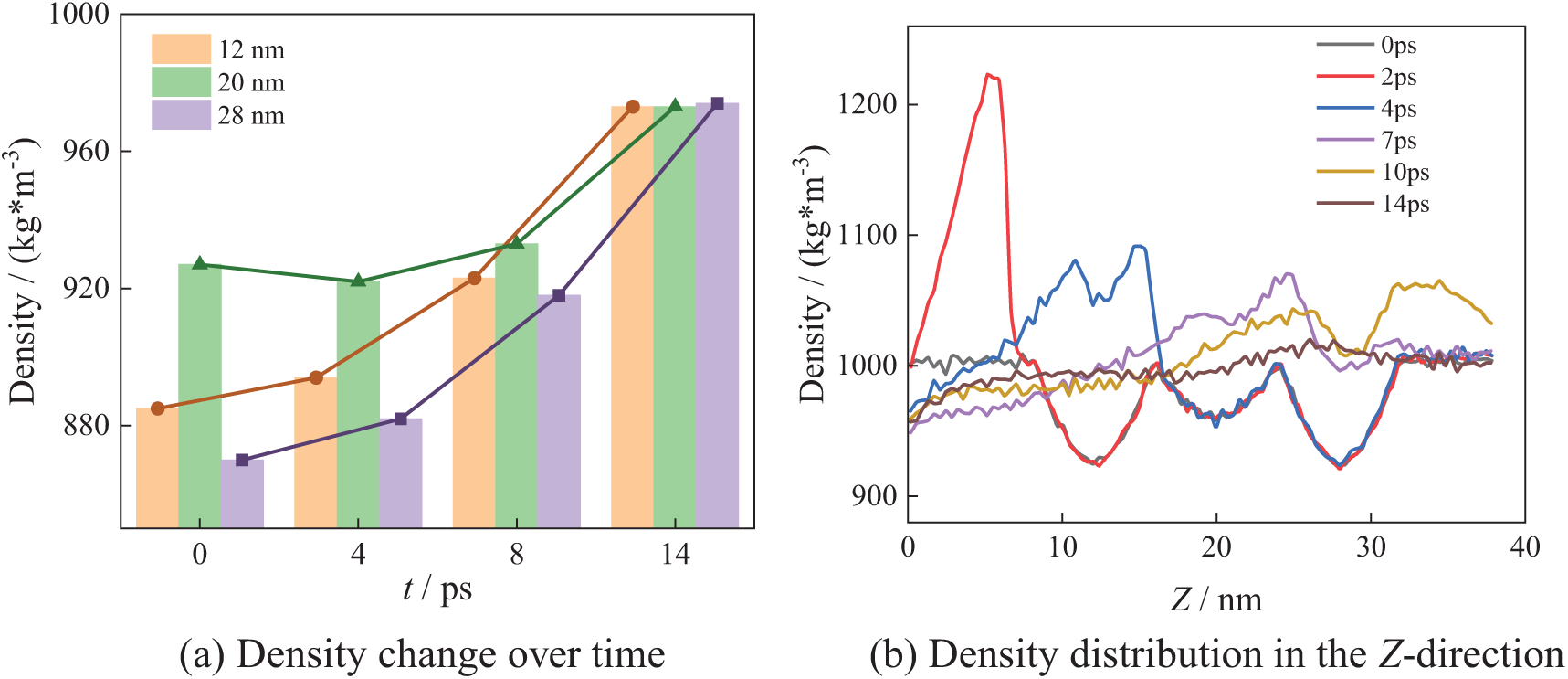
Figure 14: N_5 collapse process

As shown in Fig. 14a, at X = 12 nm and X = 28 nm, the density gradually increases during the bubble collapse until it reaches the theoretical density of water. At X = 20 nm, with the bubble collapse, the density initially decreases slightly during the collapse and then gradually increases until returning to the theoretical density of water. From Fig. 14b, it can be seen that at 2 ps, the maximum water density in the Z-direction is 1220 kg/m3. By 10 ps, the maximum density decreases to 1060 kg/m3. After bubbles collapse completely, the system density gradually returns to the theoretical density.

Fig. 15 shows the bubble collapse process in the N_7 arrangement. Similarly, there are regions of low density at the center of bubbles, i.e., 12, 24 and 36 nm. Fig. 15b shows the density distribution along the Z-direction. Three low-density regions exist at 6, 18, and 30 nm with the highest density occurring at 30 nm. These low-density regions correspond to the centers of the seven bubbles.

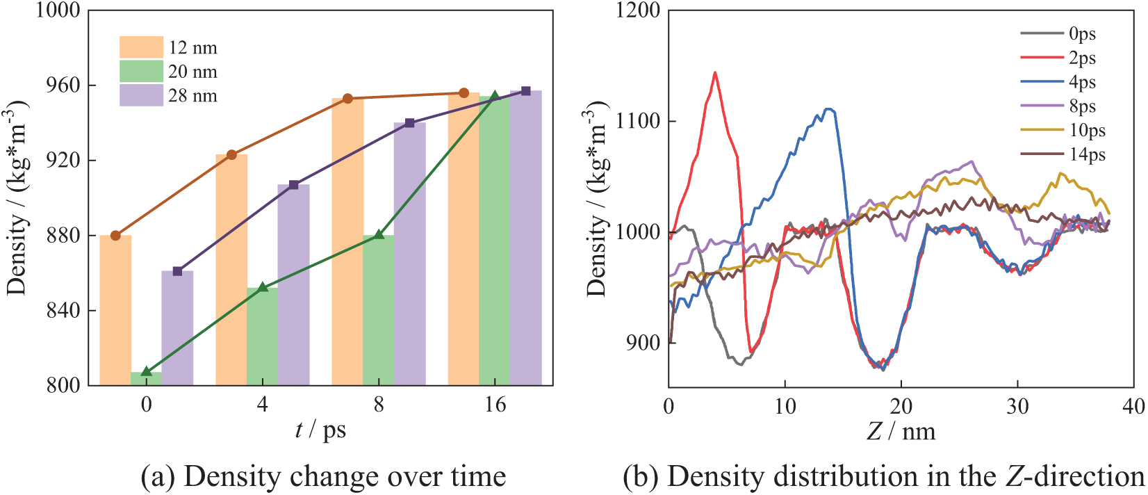
Figure 15: N_7 collapse process

As shown in Fig. 15a, the density at X = 12 nm and X = 28 nm initially increases rapidly but slows down in the later stages. In contrast, the density at X = 20 nm exhibits a faster change throughout the collapse, with the rate of change being highest in the later stage. From Fig. 15b, it can be seen that at 2 ps, the maximum density of water is 1140 kg/m3 in the Z-direction. At 15 ps, the maximum density decreases to 1050 kg/m3. After bubbles collapse completely, the system density is gradually restored to the theoretical density.

Fig. 16 shows the bubble collapse process in the N_9 arrangement. Similarly, there are regions of low density at the center of bubbles, i.e., 12, 24 and 36 nm. Fig. 16b shows the density distribution along the Z-axis direction, with three low-density regions located near 6, 18 and 30 nm, corresponding to the centers of the nine bubbles.

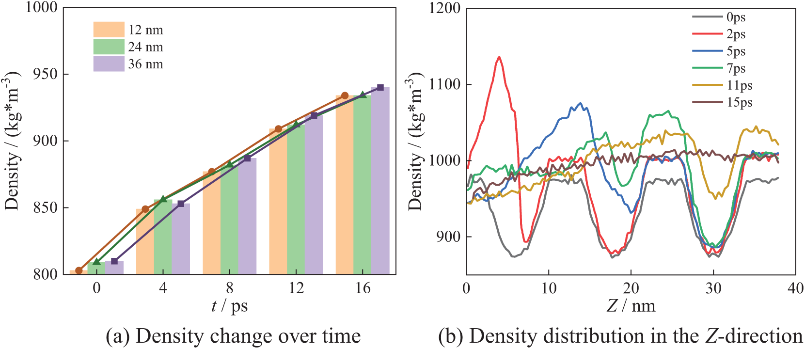
Figure 16: N_9 collapse process

As shown in Fig. 16a, it can be seen that the density gradually increases with bubble collapse at X = 12 nm, X = 24 nm, and X = 36 nm until it reaches the theoretical density of water. The local density at X = 12 nm changes more rapidly. From Fig. 16b, it can be seen that at 2 ps, the maximum density of water is 1140 kg/m3 in the Z-direction. By 10 ps, the maximum density in the Z-direction decreases to 1050 kg/m3. After bubbles collapse completely, the system density gradually returns to the theoretical density of water.

3.3 The System Pressure Analysis of the Multi-Bubble Collapse Process

3.3.1 The Odd-Numbered Bubbles and Their Arrangement on the System Pressure

Fig. 17 shows the system pressure changes of the three-bubble system under the N3_A, N3_B, and N3_C. The system pressure (P) comprises the total pressure generated by the shock wave (P1), the pressure released by the bubble collapse (P2), and the pressure of the water molecules (P3), as shown in Eq. (8):

P=P1+P2−P3(8)

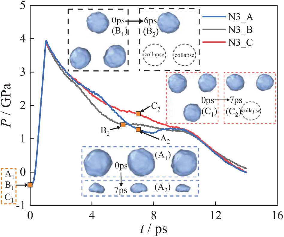
Figure 17: System pressure change of the three-bubble collapse

From Fig. 17, during the time range of 0–1 ps, the shock wave transmission causes an increase in system pressure. After 2 ps, the shock wave effect ceases, indicating the disappearance of P1. Between 2–10 ps, the system pressure is influenced only by P2 and P3. The system pressures for the N3_A, N3_B, and N3_C exhibit differences during this period.

In Fig. 17, the system pressure drops slowly, indicating that the energy released by the bubble collapse counteracts part of the resistance of the water molecules. Among the models, the system pressure in the N3_C arrangement decreases the slowest, followed by N3_A arrangement, while the N3_B arrangement exhibits the fastest pressure drop. It indicates that the pressure released by the bubble in the N3_C model is the largest under the same conditions. At the initial stage, the system pressure curve for N3_A declines the slowest, indicating that bubbles in the N3_A arrangement are the easiest to collapse and release the most energy early in the process. As the collapse progresses, the energy released by bubbles in N3_A decreases and is eventually surpassed by the energy released by bubbles in N3_B and N3_C.

3.3.2 The Even-Numbered Bubbles and Their Arrangement on the System Pressure

Subsequently, this study examines the system pressure changes in the four-bubble system under the N4_A, N4_B, N4_C, and N4_D. As shown in Fig. 18, shock wave transmission during the 0–1 ps period causes an increase in system pressure. In the time range of 2–10 ps, the system pressure changes of the four arrangements show differences, while in other moments, the pressure change trends are similar and consistent with those observed in Fig. 16. The difference is that the overall slowing down of the four-bubble system is slightly higher, indicating that the four-bubble releases more energy.

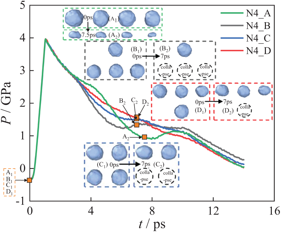
Figure 18: System pressure change of the four-bubble collapse

At the beginning of the collapse stage, the system pressure curve for N4_A decreases the most slowly, indicating that bubbles in the N4_A arrangement are the easiest to collapse at the start and release the most energy. As the collapse progresses, the energy released by the bubbles in the N4_A decreases and is eventually surpassed by the energy released by bubbles in the N4_B, N4_C, and N4_D. In contrast, the system pressure curve for N4_B drops the fastest at the beginning, indicating that bubbles in the N4_B release the least energy during the initial collapse stage. For N4_A, a significantly low-pressure value is observed near 8 ps, as all bubbles collapse at this time. Under the N4_B, N4_C and N4_D, it can be seen that there is a certain difference in the trend of the system pressure drop near 6 ps. This is because, the more bubbles collapsed, the greater the change in system pressure.

3.3.3 The Odd-Numbered Multi-Bubbles on System Pressure

Fig. 19 shows the system pressure change for the multi-bubble system under the N_5, N_7, and N_9. Shock wave transmission increases the system pressure at 0–1 ps. Between 2–10 ps, the pressure changes of the three exhibit differences, while at other moments, the pressure change trends are generally similar. Under the N_7 and N_9, the system pressure drops and then rises. This is because, there are three bubbles in the system that have collapsed at 4 ps. Near 10 ps, the red curve is flatter compared to the blue curve. This difference arises from the varying numbers of bubbles collapsing, as a greater number of collapsing bubbles produces more significant pressure changes.

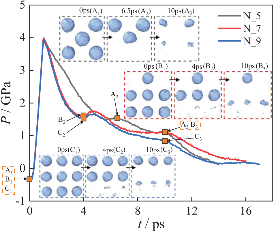
Figure 19: System pressure change of multi-bubble collapse

4  Conclusions

This paper employs the molecular dynamics simulation to study the shockwave-induced multi-bubble collapse and its development and evolution process, revealing the change laws of bubble dynamic morphology, local density distribution, and system pressure. The conclusions are as follows:

(1) The collapse speed of two sides bubbles is greater than that of the middle bubble, and their collapse time is shorter than that of the middle one. The non-uniform symmetric distribution of the bubbles affects the energy released by bubble collapse, leading to shorter collapse time.

(2) Based on the rate of pressure drop in the system, there is: N3_C＜N3_A＜N3_B. The total energy released by the bubble in N3_C is the largest, with minimal interactions between bubbles. Initially, the pressure curve of N3_A decreases the slowest, indicating that bubbles in this configuration release the most energy early in the process. Over time, the energy released by N3_A is gradually surpassed by N3_B and N3_C.

(3) At the start of collapse, the system pressure curve of N4_A decreases the slowest, and bubbles in this configuration release the most energy at this stage. However, the energy released by N4_A is eventually exceeded by that of N4_B, N4_C, and N4_D. The N4_B pressure curve decreases the fastest, indicating that bubbles in this configuration release the least energy.

(4) As the number of collapsing bubbles increases, the changes in system pressure become more pronounced. A greater number of bubbles results in more energy being released. However, the interaction between bubbles does not correlate positively with the total energy released.

Acknowledgement: Not applicable.

Funding Statement: This work is funded by the Natural Science Foundation of China [U20A20292], Shandong Province Science and Technology SMES Innovation Ability Improvement Project [2023TSGC0005], China Postdoctoral Science Foundation [2024M752697].

Author Contributions: Study conception and design, Qingjiang Xiang, Zechen Zhou; writing—original draft preparation, Xiuli Wang, Shuaijie Jiang; writing—review and editing, Zechen Zhou, Shuaijie Jiang; funding acquisition and supervision, Wei Xu, Qingjiang Xiang; investigation, Wenzhuo Guo. All authors reviewed the results and approved the final version of the manuscript.

Availability of Data and Materials: The data that support the findings of this study are available from the corresponding author upon reasonable request.

Ethics Approval: Not applicable.

Conflicts of Interest: The authors declare no conflicts of interest to report regarding the present study.

Nomenclature

N3_A	Model of three bubbles arranged in “⇀”
N3_B	Model of three bubbles arranged in “△”
N3_C	Model of three bubbles arranged in “▽”
N4_A	Model of four bubbles arranged in “⇀”
N4_B	Model of four bubbles arranged in “△”
N4_C	Model of four bubbles arranged in “◻”
N4_D	Model of four bubbles arranged in “▽”
N_5	Model of five bubbles arranged in “”
N_7	Model of seven bubbles arranged in “”
N_9	Model of nine bubbles arranged in “◻”
A*	Cross sectional area through the center of the bubble
P	Pressure of the system
USW	Total Stillinger-Weber potential energy
ULJ	Total Lennard-Jones potential energy

References

1. Zhan Q, Shi X, Fan D, Zhou L, Wei S. Solvent mixing generating air bubbles as a template for polydopamine nanobowl fabrication: underlying mechanism, nanomotor assembly and application in cancer treatment. Chem Eng J. 2021;404:126443. doi:10.1016/j.cej.2020.126443. [Google Scholar] [CrossRef]

2. Rosselló JM, Ohl CD. On-demand bulk nanobubble generation through pulsed laser illumination. Phys Rev Lett. 2021;127(4):044502. doi:10.1103/PhysRevLett.127.044502. [Google Scholar] [PubMed] [CrossRef]

3. Rezaee S, Kadivar E, El Moctar O. Molecular dynamics simulations of a nanobubble’s collapse-induced erosion on nickel boundary and porous nickel foam boundary. J Mol Liq. 2024;397:124029. doi:10.1016/j.molliq.2024.124029. [Google Scholar] [CrossRef]

4. Xu L, Yao, Shen Y. Dynamic modeling of cavitation bubble clusters: effects of evaporation, condensation, and bubble–bubble interaction. Chin Phys B. 2024;33(4):044702. doi:10.1088/1674-1056/ad181f. [Google Scholar] [CrossRef]

5. Igarashi D, Yee J, Yokoyama Y, Kusuno H, Tagawa Y. The effects of secondary cavitation position on the velocity of a laser-induced microjet extracted using explainable artificial intelligence. Phys Fluids. 2024;36(1):013317. doi:10.1063/5.0183462. [Google Scholar] [CrossRef]

6. Xu W, Jiang X, Zhao Y, Wang X, Lu Y, Lu J. Analysis of the influence of ions on degradation of benzamide with hydrodynamic cavitation technology. J Mol Liq. 2024;399:124356. doi:10.1016/j.molliq.2024.124356. [Google Scholar] [CrossRef]

7. Xu W, Zhao Y, Wang X, Lu J. Effect of shock-wave-mediated collapse on nanobubble characteristics. Langmuir. 2024;40(1):426–38. doi:10.1021/acs.langmuir.3c02679. [Google Scholar] [PubMed] [CrossRef]

8. Phan TH, Kadivar E, Nguyen VT, El Moctar O, Park WG. Thermodynamic effects on single cavitation bubble dynamics under various ambient temperature conditions. Phys Fluids. 2022;34(2):023318. doi:10.1063/5.0076913. [Google Scholar] [CrossRef]

9. Sadighi-Bonabi R, Rezaee N, Ebrahimi H, Mirheydari M. Interaction of two oscillating sonoluminescence bubbles in sulfuric acid. Phys Rev E Stat Nonlin Soft Matter Phys. 2010;82(1 pt 2):016316. doi:10.1103/PhysRevE.82.016316. [Google Scholar] [PubMed] [CrossRef]

10. Rawat S, Mitra N. Atomistic insight into the shock-induced bubble collapse in water. Phys Fluids. 2023;35(9):097114. doi:10.1063/5.0158192. [Google Scholar] [CrossRef]

11. Wei T, Gu L, Zhou M, Zhou Y, Yang H, Li M. Impact of shock-induced cavitation bubble collapse on the damage of cell membranes with different lipid peroxidation levels. J Phys Chem B. 2021;125(25):6912–20. doi:10.1021/acs.jpcb.1c02483. [Google Scholar] [PubMed] [CrossRef]

12. Mahmud KA, Hasan F, Khan MI, Adnan A. On the molecular level cavitation in soft gelatin hydrogel. Sci Rep. 2020;10(1):9635. doi:10.1038/s41598-020-66591-9. [Google Scholar] [PubMed] [CrossRef]

13. He Y, Bi Q, Shi D. Dynamics of a single air bubble rising in a thin gap filled with magnetic fluids. Fluid Dyn Mater Process. 2011;7(4):357–70. doi:10.3970/fdmp.2011.007.357. [Google Scholar] [CrossRef]

14. Nan N, Si D, Hu G. Nanoscale cavitation in perforation of cellular membrane by shock-wave induced nanobubble collapse. J Chem Phys. 2018;149(7):074902. doi:10.1063/1.5037643. [Google Scholar] [PubMed] [CrossRef]

15. Dockar D, Gibelli L, Borg MK. Shock-induced collapse of surface nanobubbles. Soft Matter. 2021;17(28):6884–98. doi:10.1039/D1SM00498K. [Google Scholar] [PubMed] [CrossRef]

16. Adhikari U, Goliaei A, Berkowitz ML. Mechanism of membrane poration by shock wave induced nanobubble collapse: a molecular dynamics study. J Phys Chem B. 2015;119(20):6225–34. doi:10.1021/acs.jpcb.5b02218. [Google Scholar] [PubMed] [CrossRef]

17. Adhikari U, Goliaei A, Berkowitz ML. Nanobubbles, cavitation, shock waves and traumatic brain injury. Phys Chem Chem Phys. 2016;18(48):32638–52. doi:10.1039/C6CP06704B. [Google Scholar] [PubMed] [CrossRef]

18. Santo KP, Berkowitz ML. Shock wave interaction with a phospholipid membrane: coarse-grained computer simulations. J Chem Phys. 2014;140(5):054906. doi:10.1063/1.4862987. [Google Scholar] [PubMed] [CrossRef]

19. Wu YT, Adnan A. Effect of shock-induced cavitation bubble collapse on the damage in the simulated perineuronal net of the brain. Sci Rep. 2017;7(1):5323. doi:10.1038/s41598-017-05790-3. [Google Scholar] [PubMed] [CrossRef]

20. Nomura KI, Choubey A, Vedadi M, Kalia RK, Nakano A, Vashishta P. Poration of lipid bilayers by shock-induced nanobubble collapse. Biophys J. 2012;102(3):729a. doi:10.1016/j.bpj.2011.11.3957. [Google Scholar] [CrossRef]

21. Hong SN, Mun SY, Ho YM, Yu CJ. Effective cracking of heavy crude oil by using shock-induced nanobubble collapse: a molecular dynamics study. J Mol Liq. 2024;414:126215. doi:10.1016/j.molliq.2024.126215. [Google Scholar] [CrossRef]

22. Vedadi M, Choubey A, Nomura K, Kalia RK, Nakano A, Vashishta P, et al. Structure and dynamics of shock-induced nanobubble collapse in water. Phys Rev Lett. 2010;105(1):014503. doi:10.1103/PhysRevLett.105.014503. [Google Scholar] [PubMed] [CrossRef]

23. Chen L, Chen PF, Li ZZ, He YL, Tao WQ. The study on interface characteristics near the metal wall by a molecular dynamics method. Comput Fluids. 2018;164:64–72. doi:10.1016/j.compfluid.2017.03.013. [Google Scholar] [CrossRef]

24. Farhadi B, Zabihi F, Yang S, Lugoloobi I, Liu A. Carbon doped lead-free perovskite with superior mechanical and thermal stability. Mol Phys. 2022;120(6):e2013555. doi:10.1080/00268976.2021.2013555. [Google Scholar] [CrossRef]

25. Fernandes HS, Sousa SF, Cerqueira NMFSA. VMD store—a VMD plugin to browse, discover, and install VMD extensions. J Chem Inf Model. 2019;59(11):4519–23. doi:10.1021/acs.jcim.9b00739. [Google Scholar] [PubMed] [CrossRef]

26. Lyubimova T, Garicheva Y, Ivantsov A. The behavior of a gas bubble in a square cavity filled with a viscous liquid undergoing vibrations. Fluid Dyn Mater Process. 2024;20(11):2417–29. doi:10.32604/fdmp.2024.052391. [Google Scholar] [CrossRef]

27. Li JB, Xu WL, Zhai YW, Luo J, Wu H, Deng J. Influence of multiple air bubbles on the collapse strength of a cavitation bubble. Exp Therm Fluid Sci. 2021;123:110328. doi:10.1016/j.expthermflusci.2020.110328. [Google Scholar] [CrossRef]

28. Fan L, Wang Y, Jiao K. Molecular dynamics simulation of diffusion and O2 dissolution in water using four water molecular models. J Electrochem Soc. 2021;168(3):034520. doi:10.1149/1945-7111/abf060. [Google Scholar] [CrossRef]

29. Molinero V, Moore EB. Water modeled as an intermediate element between carbon and silicon. J Phys Chem B. 2009;113(13):4008–16. doi:10.1021/jp805227c. [Google Scholar] [PubMed] [CrossRef]

30. Baidakov VG, Bryukhanov VM. Cavitation in a binary Lennard–Jones mixture: van der Waals gradient theory and molecular dynamics simulation. Phys Fluids. 2024;36(3):034114. doi:10.1063/5.0182453. [Google Scholar] [CrossRef]

31. Halonen R, Neefjes I, Reischl B. Further cautionary tales on thermostatting in molecular dynamics: energy equipartitioning and non-equilibrium processes in gas-phase simulations. J Chem Phys. 2023;158(19):194301. doi:10.1063/5.0148013. [Google Scholar] [PubMed] [CrossRef]

32. Ke Q, Gong X, Liao S, Duan C, Li L. Effects of thermostats/barostats on physical properties of liquids by molecular dynamics simulations. J Mol Liq. 2022;365:120116. doi:10.1016/j.molliq.2022.120116. [Google Scholar] [CrossRef]

33. Toxvaerd S. Energy, temperature, and heat capacity in discrete classical dynamics. Phys Rev E. 2024;109(1–2):015306. doi:10.1103/PhysRevE.109.015306. [Google Scholar] [PubMed] [CrossRef]