Experiments on the Start-Up and Shutdown of a Centrifugal Pump and Performance Prediction

1  Introduction

A closed impeller is characterized by the presence of both front and rear cover plates. Compared to semi-open and open impellers, closed impellers are more challenging to manufacture but find extensive application in centrifugal pumps [1]. Adiaconitei et al. have focused on the manufacturing processes of closed impellers in several studies, determining the optimal build orientation and complete fabrication procedures for closed impellers using selective laser melting (SLM) and laser powder bed fusion (LPBF) techniques [2,3]. Kumar et al. conducted a systematic study on the microstructure and mechanical properties of the lower surface of closed impellers during their manufacture [4]. These studies underscore the complexity involved in the manufacturing of closed impellers. Centrifugal pumps equipped with closed impellers exhibit advantages such as lower axial thrust, enhanced stability, and higher operational efficiency, making them suitable for a wide range of high-pressure fluid transportation. In normal operating conditions, centrifugal pumps typically maintain a relatively stable performance over extended periods, and this aspect has been the subject of extensive and thorough research. In contrast, the transient performance during starting and stopping processes has received comparatively less attention. The transient operational phases are inherently more complex and variable compared to steady-state conditions: Rezghi et al. conducted a study on the transient operation of pump-turbines during full load rejection in pumped storage power plants and performed optimization [5]. Choi et al. conducted numerical studies on the steady-state and transient characteristics of multiple types of heat pump systems [6]. Kan et al. studied the turbulent statistics and flow structures of water passing through a rotating axial-flow pump under different flow rate conditions [7]. Tong et al. predicted the best efficiency point of pumps operating as turbines and validated their findings using three different centrifugal pumps [8]. Jia et al. analyzed the internal flow characteristics and energy losses of pumps under both steady-state and transient conditions by varying the tip clearance and volute area under different operating conditions in multiple studies [9,10].

During abrupt starts and stops, or when rapid speed adjustments are made, the pump’s performance parameters undergo significant fluctuations, leading to transient flow phenomena within the pump. Such conditions can severely impact the safe operation of the pump. To ensure the safe operation of pumps, many scholars have conducted research in relevant areas: Kan et al. developed a novel predictive model to forecast the transient characteristics of the system during the pump power-off process [11]. Li et al. investigated the vibration characteristics of the impeller rotor in a mixed-flow pump during start-up under fluid-structure interaction and compared the experimental results with numerical simulations [12]. Liu et al. analyzed the water hammer effects in pump stations caused by power outages leading to pump shutdowns, providing evidence for the safety assessment of pump systems [13]. Therefore, it is important to carry out in-depth research on transient processes such as pump start and stop to improve the safety and reliability of pump operation.

In recent years, numerous scholars have conducted experiment and numerical simulation studies on the transient processes of pumps. Madeira et al. analyzed the transient characteristics of a turbine-self-excited induction generator (SEIG) system when the pump operates as a turbine. They developed an analytical model to characterize the operation of the SEIG, Pump as Turbine (PAT), and PAT-SEIG coupled systems. The results indicated that, with a sudden increase in resistive load, the hydraulic power and SEIG stator current remain nearly constant, but the reactive power of the SEIG increases, thereby reducing the efficiency of the PAT-SEIG system [14]. Julian et al. performed both experimental and numerical calculations to analyze the transient characteristics of mixed-flow turbines during starting. Their findings indicated that, due to the reverse rotation of vortices in the draft tube, there are significant pressure fluctuations at the guide vanes during starting, which can be mitigated by altering the starting procedure to enhance the service life of the blades [15]. Tsukamoto et al. undertook a comprehensive investigation into the transient characteristics of centrifugal pumps during the stopping process from both theoretical and experimental perspectives. They established an accurate and reliable mathematical model and compared the data obtained with corresponding experimental results. The results showed that the transient characteristics of pumps differ markedly from quasi-steady-state characteristics, primarily due to pressure pulsations and lag phenomena within the pump [16].

Antoine et al. utilized the bond graph method to construct a numerical model, which they analyzed dimensionlessly. They identified three consecutive stages during the rapid starting of centrifugal pumps, providing time nodes for each stage, and observed that variations in the angular acceleration of the impeller lead to increased transient effects [17]. Shourkaei employing a theoretical approach, analyzed the transient characteristics of TRR pumps during stopping. The analysis showed that both flow velocity and rotational speed exhibit a decreasing trend during stopping, with the rate of decrease gradually diminishing over time. Additionally, dynamic characteristic curves for the pump were derived based on the theoretical analysis [18].

In the investigation of pump transient characteristics, numerous scholars have utilized a variety of predictive models to forecast pump performance. Khorsheed et al. proposed an effective predictive maintenance approach using various machine learning models to detect pump bearing faults before they occur, thereby reducing downtime. Experimental results demonstrated that the multiple machine learning models employed performed well and met the expected standards [19]. Orrù et al. provided a detailed description of the development of a new machine learning model based on Support Vector Machines (SVM) and Multi-Layer Perceptrons (MLP) for early fault prediction in centrifugal pumps. The results showed that the model could accurately detect trends deviating from normal operational behavior, exhibiting good predictive accuracy [20]. Shin et al. developed and validated performance prediction models for air-source heat pump systems using various machine learning methods. The reliability of the prediction models was confirmed through comparison with experimental measurements [21]. Huang et al. incorporated a theoretical loss model into a backpropagation neural network, considering multiple geometric parameters and operating conditions. They then optimized the neural network structure by automatically determining the number of hidden layer nodes, proposing a hybrid neural network to predict the hydraulic performance of centrifugal pumps. The results showed that, for multiple centrifugal pumps, the hybrid neural network outperformed traditional linear regression over a wide range of flow rates [22]. Mohanraj et al. reviewed the application of artificial neural networks (ANNs) in the energy and exergy analysis of heat pump systems, summarizing multiple published articles in the field. The review concluded that ANNs can be successfully applied in the realm of refrigeration, air conditioning, and heat pump (RACHP) systems with acceptable accuracy [23]. Thanapandi et al. extended a performance prediction model for volute-type centrifugal pumps to also predict the dynamic characteristics during starting and stopping. In nearly all test cases, the model-predicted dynamic head-capacity curves were in excellent agreement with the experimental data [24]. Barbarelli et al. developed a one-dimensional numerical code to predict the performance of pumps operating as turbines and to determine the characteristic curves of the turbines. They compared the predicted values with experimental data from other researchers to establish the reliability of their method. The results indicated that the prediction errors were within the range of 5% to 20% [25]. Abdalla et al. investigated a predictive maintenance method for electric submersible pumps (ESPs) using extreme gradient boosting trees to analyze real-time data and predict ESP failures. Compared to traditional ESP diagnostic methods, their approach was able to identify deeper functional relationships and forecast longer-term trends [26].

Panda et al. conducted condition monitoring and fault diagnosis of centrifugal pumps based on vibration analysis, employing a support vector machine (SVM) machine learning algorithm for fault classification at different rotational speeds. The results demonstrated that the SVM algorithm performs well in this domain and application [27]. Zhang et al. proposed inverse methods for centrifugal pump blade reconstruction based on Bayesian theory, using both single-output Gaussian process regression (SOGPR) and multi-output Gaussian process regression (MOGPR). They evaluated and compared the reliability and accuracy of the two inverse problem models, and the results indicated that both models could accurately reconstruct the blade shapes within the sample space [28]. Li et al. developed a gradient boosting regression tree model to predict tobacco yield. They conducted a predictive analysis for the 2022 tobacco yield and compared it with the actual 2022 tobacco yield in China. The results showed that the gradient boosting regression tree model could accurately predict the yield [29]. Pei et al. optimized the efficiency at the design point of centrifugal pumps using an artificial neural network (ANN), constructing a precise nonlinear function between the optimization objectives and the impeller design variables. The results indicated that the use of a feedforward network for optimization improved the pump efficiency by 0.454% [30]. Wen et al. proposed and validated a deep learning neural network (DNN) trained with a back-propagation algorithm. Under the condition of specifying all design parameters, the proposed DNN was able to instantly quantify the output voltage of an HTS generator, achieving an overall accuracy of approximately 98% compared to simulated values [31]. Monstein et al. utilized generalized additive models (GAMs) to determine the appropriate structure for aerodynamic models developed from flight test data. They demonstrated the applicability of this approach using a simple pitch moment coefficient model [32].

This paper will conduct experiments on the starting and stopping processes of a 5-bladed closed impeller centrifugal pump in both power frequency and frequency conversion modes. The external characteristic parameters will be measured at various steady-state flow ratios, including head, flow rate, and rotational speed et al. A comparative analysis of the transient characteristics in the two modes will be performed to elucidate the similarities and differences in the transient characteristics of the centrifugal pump between power frequency and frequency conversion operations. Additionally, this research will employ eight different machine-learning methods to forecast the external characteristic parameters of the pump at a specific steady-state flow ratio. The aim is to identify the most accurate predictive model, which can subsequently serve as a reference for further studies on the external characteristics of other pumps.

2  Experimental Facility and Pump Model

2.1 Experimental Facility

The experimental setup for the transient performance testing of the centrifugal pump’s external characteristics, as depicted in Fig. 1, is consistent with that described in reference [33]. The setup primarily consists of a centrifugal pump unit, a testing system, a water tank, and a recirculating pipeline system. The test pump is driven by an 80M2-4 three-phase asynchronous AC motor with a rated power of 750 W. Instantaneous pressure at the pump’s inlet and outlet is measured using WIKA S-10 pressure transmitters manufactured by WIKA Alexander Wiegand SE & Co. KG, Germany. These transducers have an inlet pressure measurement range of −1 to 1 MPa and an outlet pressure measurement range of 0 to 1.6 MPa, with an accuracy of ±25%. The instantaneous flow rate of the centrifugal pump is measured with an OPTIFLUX 2100C electromagnetic flowmeter produced by KROHNE Messtechnik (Shanghai) Co., Ltd., Shanghai, China. This device is configured with a time constant of 0.1 s, a pulse output frequency of 1 kHz, a maximum flow capacity of 30 m3/h, and an accuracy class of 0.5. The instantaneous rotational speed of the centrifugal pump is measured using a JC0 torque-speed sensor from Hunan Xiangyi Power Test Instrument Co., Ltd., Changsha, China. This sensor has a measurement range of 0 to 5 N·m, an accuracy class of 0.2, a signal sampling period of 1 ms, and an uncertainty in both speed and torque measurements of ±0.25%. An NC-3 torque meter is employed to measure the instantaneous shaft torque of the centrifugal pump, with a precision of ±0.1%. During variable frequency experiments, the power supply frequency of the motor is adjusted using a SIEMENS MICROMASTER 440 inverter manufactured by Siemens AG, Germany. All physical parameters are transmitted as 4–20 mA current signals, which are then collected via a PCI8361BN data acquisition card, produced by Beijing Zhongtai Yanchuang Technology Co., Ltd., Beijing, China.

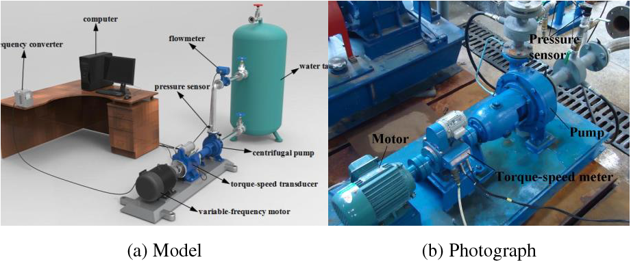
Figure 1: Test rig

2.2 Experimental Pump

The experimental pump is a centrifugal pump featuring a closed impeller with five blades, designed with the following parameters: a flow rate of 6 m3/h, a head of 8 m, and an rotational speed of 1450 rpm. The blade profile is characterized as a two-dimensional, bi-circular cylindrical shape, and the impeller consists of five such blades. The variation in the volute dimensions follows an Archimedean spiral pattern. The principal geometric dimensions of the model pump’s volute and impeller are detailed in Table 1. A three-dimensional sectional view of the centrifugal impeller, along with its dimensional specifics, is illustrated in Fig. 2.

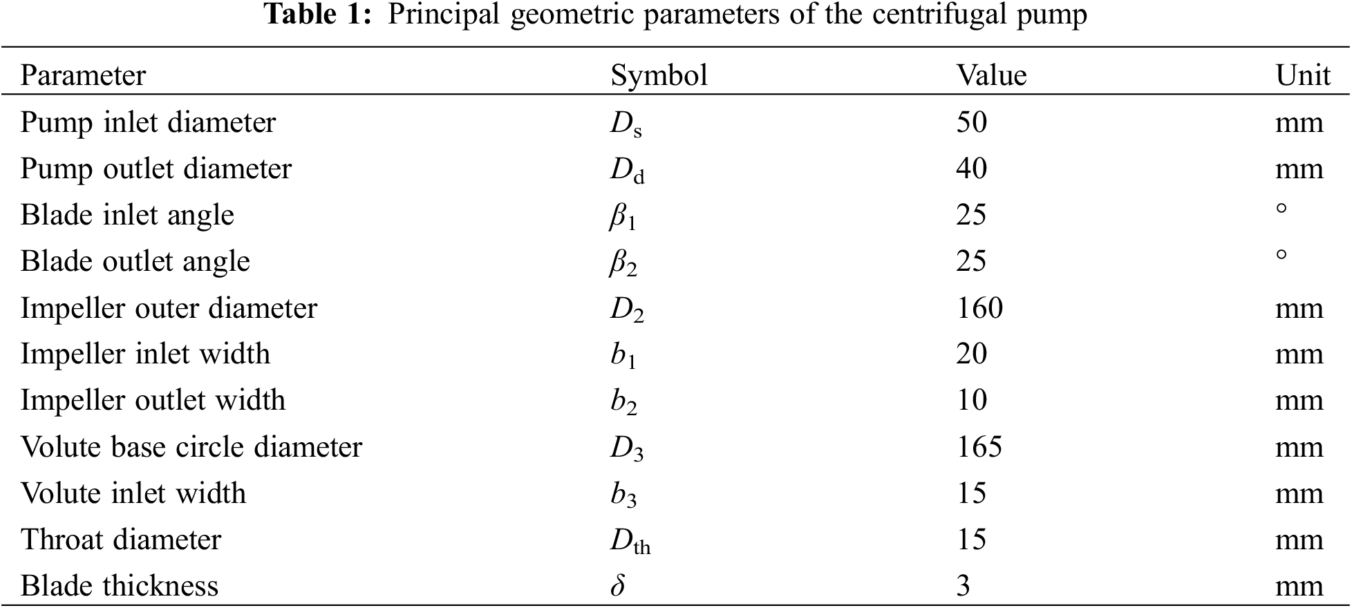
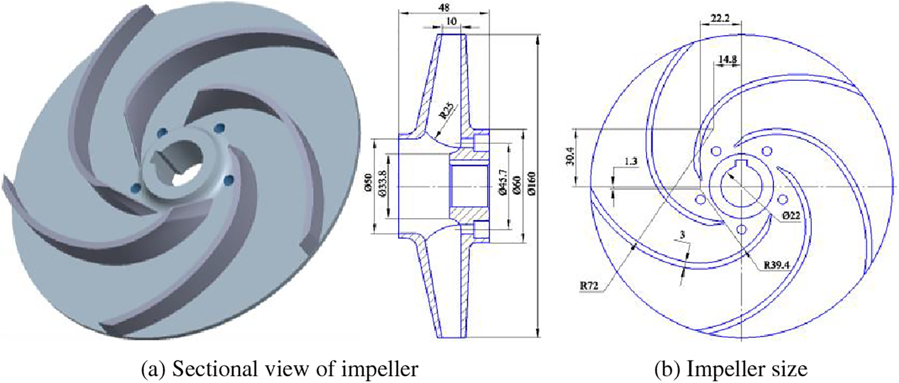
Figure 2: Centrifugal impeller

In this study, the starting experiments will be conducted in two operational models: power frequency and frequency conversion. The power frequency model refers to the standard alternating current (AC) power supply frequency used in industry, which is a constant 50 Hz. In contrast, the frequency conversion model involves the adjustment of the supply frequency through a variable frequency drive (VFD), enabling the regulation of the motor’s rotational speed.

The distinction between the two starting methods is significant. During power frequency start, the motor is directly connected to the power grid and operates at the fixed frequency supplied by the grid. This method allows for a very rapid startup and quick response. However, it results in a starting current that can be 7 to 8 times the motor’s rated current, potentially causing a significant impact on the electrical grid, leading to voltage drops and affecting the normal operation of other electrical equipment. Additionally, the high starting current imposes substantial electrical stress on the motor windings, thereby reducing the motor’s lifespan.

In contrast, frequency conversion startup utilizes a VFD to control the input power frequency to the motor, enabling a smooth and gradual start. This not only allows for continuous adjustment of the motor speed but also significantly reduces the starting current and mechanical wear during startup. As a result, the impact on both the grid and the equipment is minimized. Nevertheless, compared to power frequency, frequency conversion startup has a slower response time and requires higher maintenance costs.

3  Analysis of Experimental Results

3.1 Starting Process

Fig. 3 illustrates the variations in inlet pressure of the experimental pump in two modes. Specifically, Fig. 3a shows the changes in inlet pressure during starting for the pump operating at power frequency mode with steady-state flow rate ratios of Q/Qr = 0.311, 0.515, 0.709, 0.905, 1.108, and 1.308. Fig. 3b presents the corresponding inlet pressure changes during starting for the pump operating at frequency conversion mode with steady-state flow rate ratios of Q/Qr = 0.307, 0.509, 0.697, 0.897, 1.098, and 1.296.

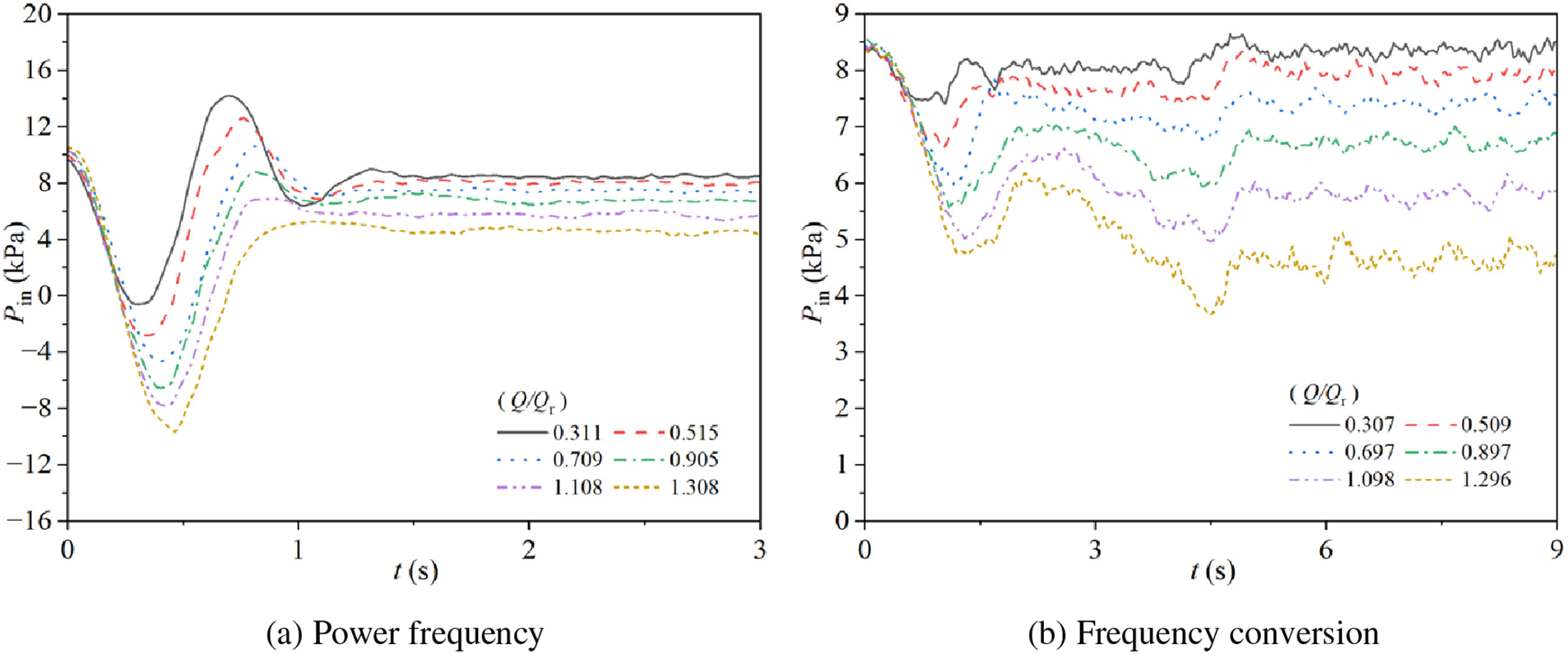
Figure 3: Inlet pressure characteristics for two modes

During the power frequency starting, the inlet pressure changes for the pump at six different valve openings all exhibit a pattern of an initial rapid decrease, followed by a rapid increase, another rapid decrease, and finally stabilization. As the steady-state flow rate ratio increases, the inlet pressure curves reach their respective valley values at t = 0.31, 0.36, 0.41, 0.42, 0.42, and 0.47 s, with corresponding pressure values of −0.57, −2.81, −4.69, −6.49, −7.80, and −9.64 kPa. Subsequently, the curves reach their peak values at t = 0.69, 0.77, 0.81, 0.81, 0.89, and 1.08 s, with pressures of 14.18, 12.60, 10.60, 8.78, 6.88, and 5.25 kPa, respectively. The pressures then stabilize at t = 1.44, 1.52, 1.23, 1.11, 1.05, and 0.97 s, with final stable values of 8.51, 8.25, 7.45, 6.44, 5.97, and 5.07 kPa, respectively.

As the steady-state flow rate ratio increases, the peak-to-valley, and stable values of the inlet pressure all gradually decrease. Additionally, the times at which the peak-to-valley values are reached are slightly delayed as the steady-state flow rate ratio increases, while the time to reach the stable value is gradually advanced. For steady-state flow rate ratios of Q/Qr = 0.311, 0.515, and 0.709, there are small fluctuations in the inlet pressure before reaching the stable value. In contrast, for Q/Qr = 0.905, 1.108, and 1.308, the inlet pressure gradually stabilizes. Overall, as the steady-state flow rate ratio increases, the fluctuations in the inlet pressure before reaching the stable value tend to diminish.

Regardless of the valve opening, during frequency conversion starting, the inlet pressure of the pump generally exhibits a pattern of initially decreasing, then increasing, followed by another decrease, and finally stabilizing over time. As the steady-state flow rate ratio increases, the curves reach their respective valley values at t = 0.75, 1.02, 1.13, 1.25, 1.30, and 1.33 s, with corresponding pressure values of 7.47, 6.58, 5.98, 5.60, 5.01, and 4.73 kPa. Subsequently, the curves reach their peak values at t = 1.34, 1.78, 1.69, 2.00, 2.14, and 2.11 s, with pressures of 8.19, 7.85, 7.83, 6.99, 6.44, and 6.15 kPa, respectively. The curves then reach a second set of valley values at t = 4.14, 4.13, 4.39, 4.39, 4.50, and 4.53 s, with pressures of 7.77, 7.45, 6.77, 5.94, 4.96, and 3.70 kPa, respectively. Finally, the inlet pressure stabilizes at t = 5.05, 5.09, 5.11, 5.06, 5.02, and 4.92 s, with stable values of 8.44, 8.12, 7.53, 6.81, 5.80, and 4.72 kPa, respectively.

As the steady-state flow rate ratio increases, the peak-to-valley and stable values of the inlet pressure all gradually decrease. Additionally, the times at which the peak-to-valley values are reached are slightly delayed as the steady-state flow rate ratio increases. The fluctuations before reaching the stable value, however, tend to increase.

The stable values of the pump inlet pressure for each steady-state flow rate ratio are generally consistent between the two modes. However, power frequency mode reaches the stable value more quickly compared to frequency conversion mode. In contrast, frequency conversion mode exhibits smaller pressure fluctuations before reaching the stable value compared to power frequency mode.

As the steady-state flow rate ratio increases, the pressure fluctuations before reaching the stable value during power frequency mode gradually decrease. Conversely, the pressure fluctuations before reaching the stable value during frequency conversion mode gradually increase with the increase in the steady-state flow rate ratio.

Fig. 4 illustrates the variations in outlet pressure of the experimental pump in two starting modes. Specifically, Fig. 4a shows the changes in outlet pressure during starting for the pump operating at power frequency mode with steady-state flow rate ratios of Q/Qr = 0.311, 0.515, 0.709, 0.905, 1.108, and 1.308. Fig. 4b presents the corresponding outlet pressure changes during starting for the pump operating at frequency conversion mode with steady-state flow rate ratios of Q/Qr = 0.307, 0.509, 0.697, 0.897, 1.098, and 1.296.

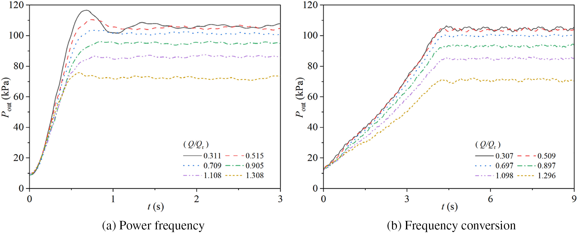
Figure 4: Outlet pressure characteristics for two modes

During power frequency starting, the outlet pressure for the six different steady-state flow rate ratios exhibits a trend of initially increasing rapidly and then stabilizing. For the steady-state flow rate ratio Q/Qr = 0.311, the curve reaches its peak value of 116.62 kPa at t = 0.69 s, then drops to a valley value of 101.82 kPa at t = 1.02 s, and finally stabilizes at 106.40 kPa at t = 1.25 s. For Q/Qr = 0.515, the curve reaches its peak value of 110.50 kPa at t = 0.73 s and stabilizes at 105.60 kPa at t = 1.03 s. The other curves stabilize at 102.79, 94.76, 85.11, and 74.52 kPa at t = 0.70, 0.78, 0.72, and 0.64 s, respectively, as the steady-state flow rate ratio increases.

As the steady-state flow rate ratio increases, the stable values of the outlet pressure gradually decrease, and the time to reach the stable value slightly advances. For Q/Qr = 0.311 and 0.515, there are small fluctuations in the outlet pressure before reaching the stable value, while for Q/Qr = 0.709, 0.905, 1.108, and 1.308, the outlet pressure gradually stabilizes. Overall, as the steady-state flow rate ratio increases, the fluctuations before reaching the stable value tend to diminish, and the rate of decrease in the stable outlet pressure values also accelerates.

For the six different steady-state flow rate ratios tested, the outlet pressure during frequency conversion starting generally shows an initial increase followed by stabilization. As the steady-state flow rate ratio increases, the curves reach their respective stable values of 104.52, 102.90, 99.58, 92.72, 84.29, and 70.49 kPa at t = 4.28, 4.14, 4.27, 4.30, 4.27, and 4.19 s, respectively. As the steady-state flow rate ratio increases, the stable values of the outlet pressure gradually decrease, and the rate of decrease in the stable values also accelerates.

In summary, the stable values of the outlet pressure during power frequency starting are slightly higher than those during frequency conversion starting. Power frequency starting reaches the stable value more quickly, whereas frequency conversion starting exhibits smaller pressure fluctuations before reaching the stable value.

Fig. 5 illustrates the variations in head of the experimental pump in two starting modes. Specifically, Fig. 5a shows the changes in head during starting for the pump operating at power frequency mode with steady-state flow rate ratios of Q/Qr = 0.311, 0.515, 0.709, 0.905, 1.108, and 1.308. Fig. 5b presents the corresponding head changes during starting for the pump operating at frequency conversion mode with steady-state flow rate ratios of Q/Qr = 0.307, 0.509, 0.697, 0.897, 1.098, and 1.296.

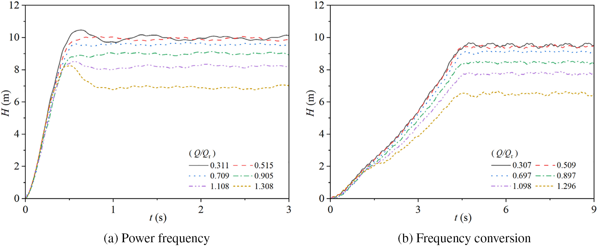
Figure 5: Head characteristics for two modes

During power frequency starting, the head for the six different steady-state flow rate ratios exhibits a trend of initially increasing rapidly and then stabilizing. For the steady-state flow rate ratio Q/Qr = 0.311, the curve reaches its peak value of 10.46 m at t = 0.63 s and then stabilizes at 9.97 m at t = 0.83 s. For Q/Qr = 1.308, the curve reaches its peak value of 8.24 m at t = 0.52 s and stabilizes at 6.89 m at t = 0.84 s. The other curves, for Q/Qr = 0.515, 0.709, 0.905, and 1.108, stabilize at 10.01, 9.52, 8.87, and 8.19 m at t = 0.67, 0.64, 0.66, and 0.72 s, respectively, after a rapid initial increase.

Overall, the stable values of the head decrease as the steady-state flow rate ratio increases. Additionally, the rate of decrease in the stable head values accelerates with increasing steady-state flow rate ratio. For Q/Qr = 0.311 and 1.308, there are small fluctuations in the head before reaching the stable value, while for Q/Qr = 0.515, 0.709, 0.905, and 1.108, the head gradually stabilizes without significant fluctuations.

During frequency conversion starting, the head of the pump gradually increases over time and then stabilizes. For the six different steady-state flow rate ratios, the head curves are nearly identical for t ≤ 1 s, but differences begin to emerge as time progresses beyond 1 s. Specifically, the head stabilizes at 9.76, 9.65, 9.39, 8.80, 8.07, and 6.67 m at t = 4.63, 4.42, 4.77, 4.64, 4.64, and 4.77 s, respectively, for Q/Qr = 0.307, 0.509, 0.697, 0.897, 1.098, and 1.296.

As the steady-state flow rate ratio increases, the stable values of the head during frequency conversion starting gradually decrease, and the magnitude of this decrease also increases.

Compared to power frequency starting, the head during frequency conversion starting takes longer to reach a stable value, and the stable values of the head are slightly lower. Additionally, the head during frequency conversion starting exhibits more stable behavior with fewer fluctuations compared to power frequency starting.

Fig. 6 illustrates the variations in flow rate of the experimental pump in two modes. Specifically, Fig. 6a shows the changes in flow rate during starting for the pump operating at power frequency mode with steady-state flow rate ratios of Q/Qr = 0.311, 0.515, 0.709, 0.905, 1.108, and 1.308. Fig. 6b presents the corresponding flow rate changes during starting for the pump operating at frequency conversion mode with steady-state flow rate ratios of Q/Qr = 0.307, 0.509, 0.697, 0.897, 1.098, and 1.296.

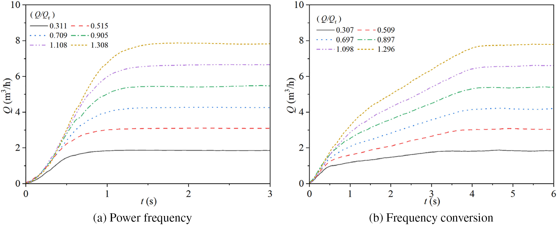
Figure 6: Flow rate characteristics for two modes

During power frequency starting, the flow rate for the six different steady-state flow rate ratios exhibits a trend of initially increasing and then gradually stabilizing. The flow rate characteristics show a two-stage change: before reaching the stable value, the flow rate increases over time, with the rate of increase first accelerating and then decelerating. As the steady-state flow rate ratio increases, the flow rate reaches its stable values of 1.84, 3.06, 4.23, 5.44, 6.59, and 7.85 m3/h at t = 1.03, 1.20, 1.39, 1.49, 1.58, and 1.69 s, respectively.

During frequency conversion starting, the flow rate characteristics for the six different steady-state flow rate ratios exhibit a three-stage pattern: the first stage is characterized by a rapid increase in flow rate, the second stage shows a slower rate of increase compared to the first stage, and the third stage is marked by the flow rate stabilizing and remaining constant. As the steady-state flow rate ratio increases, the flow rate characteristics show the following transitions: the first change in the rate of flow rate increase occurs at t = 0.53, 0.56, 0.64, 0.86, 1.20, and 1.45 s, respectively, and the second change in the rate of flow rate increase, leading to stabilization, occurs at t = 3.23, 3.80, 3.97, 4.14, 4.27, and 4.33 s, respectively. The flow rates stabilize at the following values: 1.80 m3/h for Q/Qr = 0.307, 3.00 m3/h for Q/Qr = 0.509, 4.14 m3/h for Q/Qr = 0.697, 5.36 m3/h for Q/Qr = 0.897, 6.52 m3/h for Q/Qr = 1.098, and 7.72 m3/h for Q/Qr = 1.296.

Overall, the stable values of the flow rate are similar between power frequency and frequency conversion starting. However, the flow rate during power frequency starting reaches its stable value more quickly compared to frequency conversion starting. The rate of change in flow rate during power frequency starting is continuous, while during frequency conversion starting, the rate of change in flow rate exhibits a stepwise, three-stage pattern.

Fig. 7 illustrates the variations in rotational speed of the experimental pump in two starting modes. Specifically, Fig. 7a shows the changes in rotational speed during starting for the pump operating at power frequency mode with steady-state flow rate ratios of Q/Qr = 0.311, 0.515, 0.709, 0.905, 1.108, and 1.308. Fig. 7b presents the corresponding rotational speed changes during starting for the pump operating at frequency conversion mode with steady-state flow rate ratios of Q/Qr = 0.307, 0.509, 0.697, 0.897, 1.098, and 1.296.

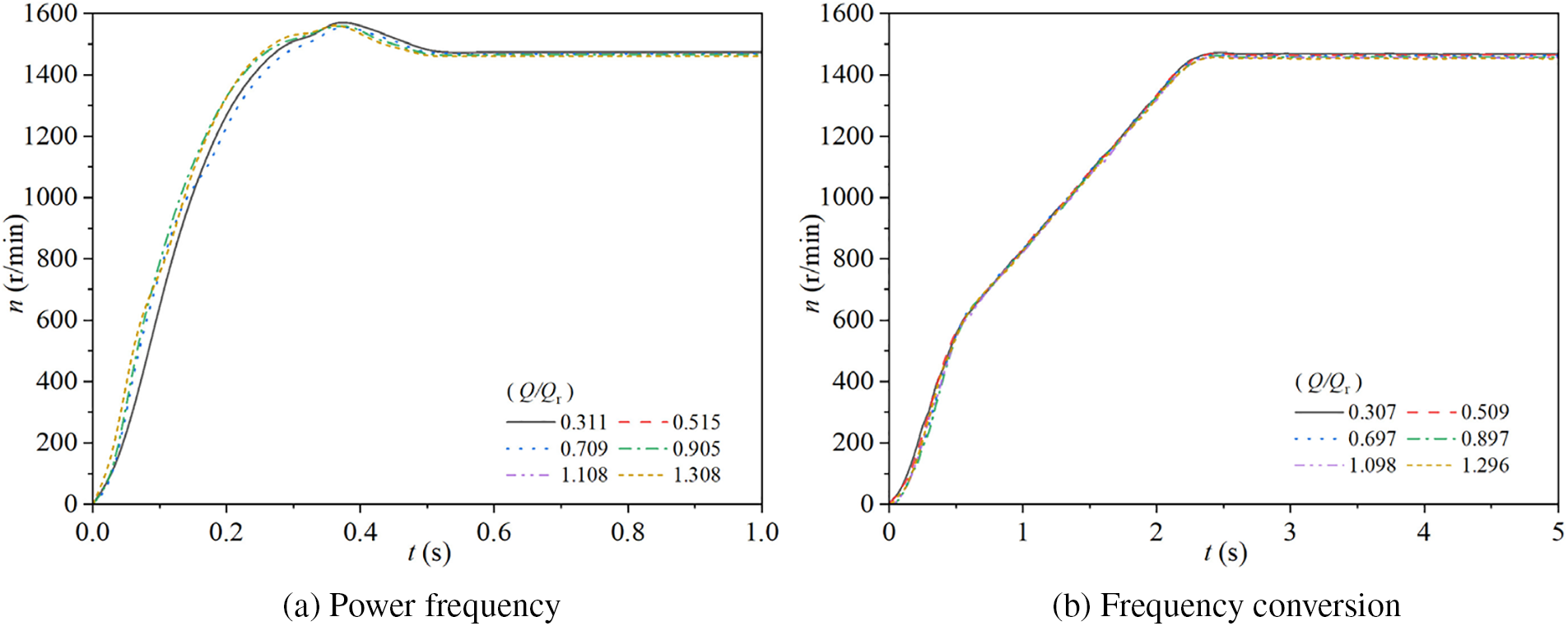
Figure 7: Rotational speed characteristics for two modes

During power frequency starting, the rotational speed characteristics do not show significant differences due to the variation in steady-state flow rate ratios. The rotational speed initially increases rapidly, then gradually slows down, and experiences a small fluctuation before reaching a peak. The peaks are reached at t = 0.36, 0.39, 0.39, 0.36, 0.38, and 0.36 s, with corresponding peak values of 1566.14, 1565.55, 1551.17, 1557.02, 1563.70, and 1560.45 r/min, respectively. After reaching the peak, the rotational speed gradually decreases and stabilizes at 1470.50 r/min at t = 0.53 s.

During frequency conversion starting, the rotational speed characteristics exhibit a three-stage pattern. For all six steady-state flow rate ratios, the rotational speed initially increases rapidly, reaches 589.55 r/min at t = 0.55 s, then the rate of increase slightly decreases, and finally stabilizes at 1470.45 r/min at t = 2.41 s.

Compared to power frequency starting, the rotational speed during frequency conversion starting takes longer to reach its stable value and exhibits a three-stage linear change. In contrast, during power frequency starting, the rate of increase in rotational speed changes before reaching the stable value, showing a trend of rapid initial increase followed by a gradual slowdown, and there is a spike in speed before stabilization, resulting in peak speeds that are higher than the stable value. In both power frequency and frequency conversion starting modes, the rotational speed characteristics show minimal dependence on the steady-state flow rate ratio. In the six different steady-state flow rate ratios tested, the rotational speed characteristic curves remain largely unchanged, indicating that the rotational speed behavior is relatively independent of the specific steady-state flow rate ratio.

Fig. 8 illustrates the variations in torque of the experimental pump in two starting modes. Specifically, Fig. 8a shows the changes in torque during starting for the pump operating at power frequency mode with steady-state flow rate ratios of Q/Qr = 0.311, 0.515, 0.709, 0.905, 1.108, and 1.308. Fig. 8b presents the corresponding torque changes during starting for the pump operating at frequency conversion mode with steady-state flow rate ratios of Q/Qr = 0.307, 0.509, 0.697, 0.897, 1.098, and 1.296.

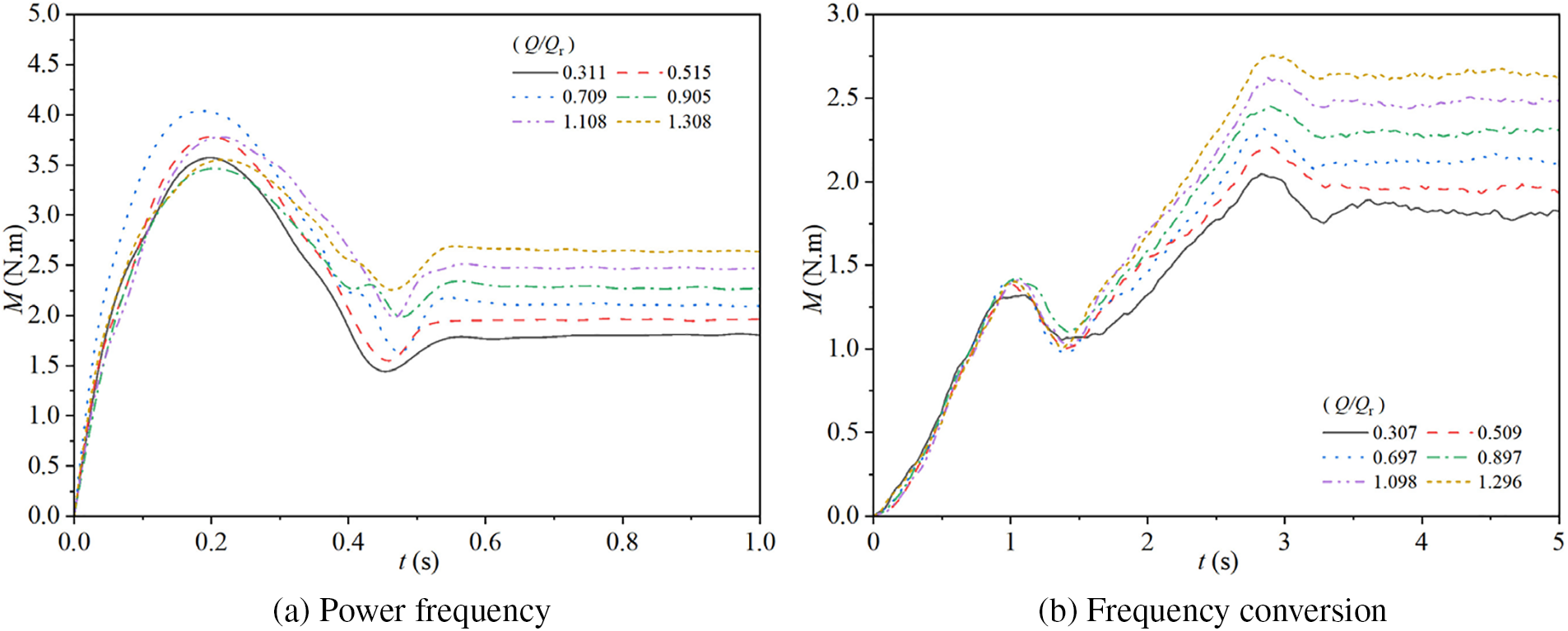
Figure 8: Torque characteristics for two modes

During power frequency starting, the torque of the pump increases rapidly, reaches a peak, then decreases quickly, followed by a brief increase, and finally stabilizes. The torque peaks for the different steady-state flow rate ratios (Q/Qr = 0.311, 0.515, 0.709, 0.905, 1.108, 1.308) are reached at t = 0.20 s with values of 3.57, 3.78, 4.02, 3.47, 3.77, and 3.54 N·m, respectively. The torque then reaches its troughs at t = 0.47, 0.47, 0.49, 0.47, 0.47, and 0.45 s, with values of 1.47, 1.57, 1.67, 2.01, 1.98, and 2.28 N·m, respectively. Finally, the torque stabilizes at t = 0.56, 0.56, 0.59, 0.63, 0.64, and 0.63 s, with stable values of 1.79, 1.95, 2.13, 2.29, 2.47, and 2.67 N·m, respectively. For Q/Qr = 0.709 and 0.905, there is an additional fluctuation at t = 0.42 s before the torque drops to the trough. With increasing steady-state flow rate ratio, the stable value of the torque increases linearly, but the times to reach the peak and trough do not change significantly with the steady-state flow rate ratio.

During frequency conversion starting, the torque initially increases, then decreases, increases again, and finally decreases to reach a stable value. The torque peaks for the different steady-state flow rate ratios (Q/Qr = 0.307, 0.509, 0.697, 0.897, 1.098, 1.296) are reached at t = 1.11, 1.00, 1.03, 1.06, 1.03, and 1.03 s, with values of 1.32, 1.38, 1.41, 1.42, 1.41, and 1.40 N·m, respectively. The torque then reaches its troughs at t = 1.38, 1.41, 1.41, 1.42, 1.45, and 1.36 s, with values of 1.05, 1.00, 0.98, 1.10, 1.02, and 1.01 N·m, respectively. After that, the torque reaches its maximum values at t = 2.83, 2.91, 2.83, 2.88, 2.88, and 2.91 s, with values of 2.05, 2.20, 2.32, 2.45, 2.62, and 2.75 N·m, respectively. Finally, the torque stabilizes at t = 3.41, 3.33, 3.28, 3.28, 3.33, and 3.27 s, with stable values of 1.82, 1.98, 2.10, 2.26, 2.46, and 2.62 N·m, respectively. As the steady-state flow rate ratio increases, the maximum and stable values of the torque also increase linearly during power frequency starting.

Overall, the torque of the pump during power frequency starting typically stabilizes around t = 0.55 s, while during frequency conversion starting, it takes longer, stabilizing around t = 3.3 s. During power frequency starting, the torque exhibits more significant fluctuations before reaching the stable value, whereas during frequency conversion starting, the torque changes are smoother.

Fig. 9 illustrates the variations in shaft power of the experimental pump in two starting modes. Specifically, Fig. 9a shows the changes in shaft power during starting for the pump operating at power frequency mode with steady-state flow rate ratios of Q/Qr = 0.311, 0.515, 0.709, 0.905, 1.108, and 1.308. Fig. 9b presents the corresponding shaft power changes during starting for the pump operating at frequency conversion mode with steady-state flow rate ratios of Q/Qr = 0.307, 0.509, 0.697, 0.897, 1.098, and 1.296.

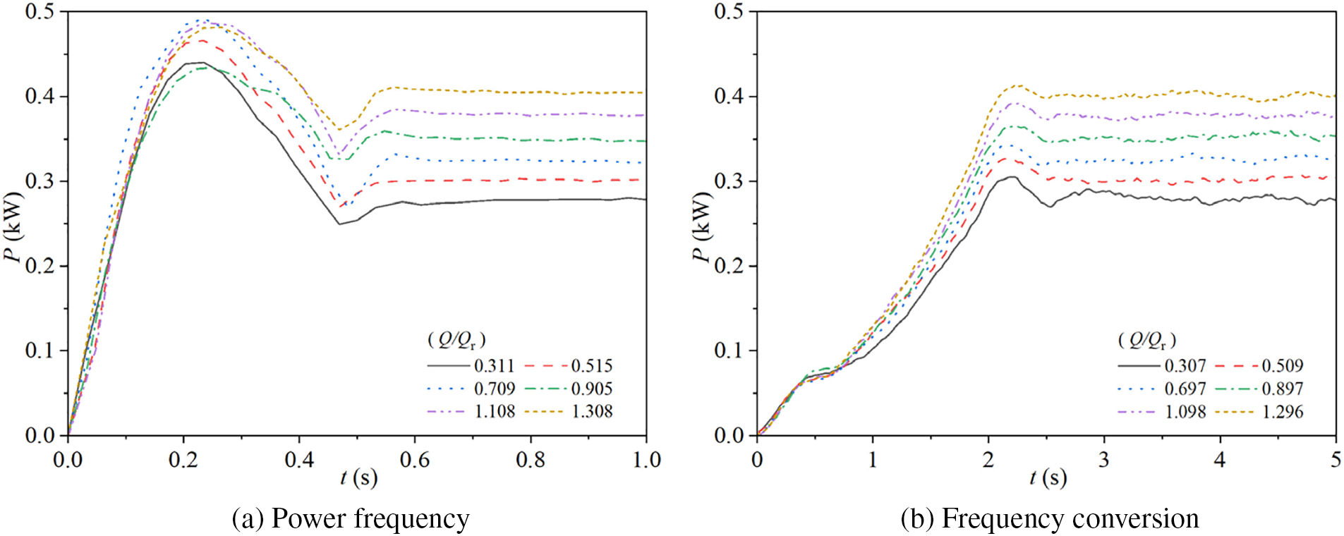
Figure 9: Shaft power characteristics for two modes

During power frequency starting, as the steady-state flow rate ratio increases, the shaft power for the six different valve openings starts from zero and increases rapidly, reaching their maximum values at t = 0.24, 0.23, 0.24, 0.25, 0.24, and 0.27 s, with values of 0.44, 0.47, 0.49, 0.43, 0.49, and 0.48 kW, respectively. The shaft power then decreases rapidly, reaching troughs at t = 0.47, 0.47, 0.49, 0.49, 0.47, and 0.47 s, with values of 0.25, 0.27, 0.27, 0.33, 0.33, and 0.36 kW, respectively. After that, the shaft power gradually increases and stabilizes at t = 0.58, 0.56, 0.66, 0.64, 0.64, and 0.59 s, with stable values of 0.28, 0.30, 0.32, 0.35, 0.38, and 0.41 kW, respectively. As the steady-state flow rate ratio increases, the stable value of the shaft power also increases linearly.

During frequency conversion starting, the shaft power of the pump exhibits a three-stage characteristic as time progresses: in the first stage from 0 s to 0.41 s, the shaft power gradually increases with time, and the rate of increase does not show significant differences across the different steady-state flow rate ratios, with all six ratios (Q/Qr = 0.307, 0.509, 0.697, 0.897, 1.098, 1.296) reaching 0.07 kW at t = 0.41 s; in the second stage from 0.41 s to 2.27 s, the shaft power continues to increase, and the rate of increase becomes more pronounced as the steady-state flow rate ratio increases, reaching maximum values at t = 2.27 s of 0.31, 0.33, 0.34, 0.36, 0.39, and 0.41 kW, respectively; in the third stage after 2.27 s, the shaft power stabilizes at t = 2.59, 2.55, 2.52, 2.59, 2.56, and 2.50 s, with stable values of 0.28, 0.30, 0.32, 0.35, 0.37, and 0.40 kW, respectively. As the steady-state flow rate ratio increases, the stable value of the shaft power during frequency conversion starting also increases linearly.

When comparing the two starting modes, it is evident that the shaft power during frequency conversion starting takes longer to reach its stable value compared to power frequency starting. However, before reaching the stable value, the magnitude of the shaft power changes over time is smaller in frequency conversion starting, and the maximum values of shaft power during starting are lower than those in power frequency starting. This indicates that the frequency conversion starting is more stable compared to power frequency starting.

3.2 Stopping Process

Fig. 10 illustrates the variations in inlet pressure of the experimental pump in two modes. Specifically, Fig. 10a shows the changes in inlet pressure during stopping for the pump operating at power frequency mode with steady-state flow rate ratios of Q/Qr = 0.311, 0.515, 0.709, 0.905, 1.108, and 1.308. Fig. 10b presents the corresponding inlet pressure changes during stopping for the pump operating at frequency conversion mode with steady-state flow rate ratios of Q/Qr = 0.307, 0.509, 0.697, 0.897, 1.098, and 1.296.

Figure 10: Inlet pressure characteristics for two modes

During power frequency stopping, the inlet pressure for the different steady-state flow rate ratios (Q/Qr = 0.311, 0.515, 0.709, 0.905, 1.108, 1.308) initially increases rapidly, reaching maximum values at t = 0.36, 0.39, 0.38, 0.44, 0.47, and 0.50 s, with values of 10.46, 10.71, 10.53, 10.63, 10.34, and 10.07 kPa, respectively. For Q/Qr = 0.311, the inlet pressure then decreases rapidly, reaching a trough at t = 0.77 s with a value of 8.33 kPa, and gradually stabilizes to a stable value of 8.74 kPa at t = 2.09 s. For the other steady-state flow rate ratios (Q/Qr = 0.515, 0.709, 0.905, 1.108, 1.308), the inlet pressure decreases more slowly after reaching the maximum, showing slightly larger fluctuations between 0.35 and 1.65 s, and then smoothly decreases to stable values of 8.82, 8.89, 8.75, 8.64, and 8.65 kPa at approximately t = 2.27, 3.83, 5.36, 6.64, and 7.03 s, respectively. As the steady-state flow rate ratio increases, the time to reach a stable inlet pressure during power frequency stopping also increases, while the fluctuations before stabilization decrease with increasing steady-state flow rate ratio.

During frequency conversion stopping, the inlet pressure for all six different steady-state flow rate ratios exhibits an initial increase followed by a gradual decrease to a stable value. For Q/Qr = 0.307, the inlet pressure reaches a maximum of 9.19 kPa at t = 0.49 s, shows slight fluctuations between 0.5 and 4.3 s, and stabilizes at 8.64 kPa at t = 4.28 s. For Q/Qr = 0.509, the inlet pressure reaches a maximum of 9.11 kPa at t = 0.52 s, shows slight fluctuations between 0.5 and 4.3 s, and stabilizes at 8.56 kPa at t = 5.72 s. For Q/Qr = 0.697, 0.897, 1.098, and 1.296, the inlet pressure reaches maxima of 9.23, 9.30, 9.29, and 9.33 kPa at t = 2.25, 2.25, 2.25, and 2.80 s, respectively, and then decreases slowly, finally stabilizing at 8.67, 8.70, 8.63, and 8.63 kPa at t = 6.83, 7.09, 7.33, and 7.47 s, respectively. As the steady-state flow rate ratio increases, the time to reach a stable inlet pressure during frequency conversion stopping also increases.

When comparing the two stopping modes, it is evident that the inlet pressure during frequency conversion stopping takes longer to stabilize compared to power frequency stopping. However, as the steady-state flow rate ratio increases, the difference in stabilization times between the two modes decreases. Additionally, the fluctuations in inlet pressure before stabilization are greater in power frequency stopping than in frequency conversion stopping.

Fig. 11 illustrates the variations in outlet pressure of the experimental pump in two modes. Specifically, Fig. 11a shows the changes in outlet pressure during stopping for the pump operating at power frequency mode with steady-state flow rate ratios of Q/Qr = 0.311, 0.515, 0.709, 0.905, 1.108, and 1.308. Fig. 11b presents the corresponding outlet pressure changes during stopping for the pump operating at frequency conversion mode with steady-state flow rate ratios of Q/Qr = 0.307, 0.509, 0.697, 0.897, 1.098, and 1.296.

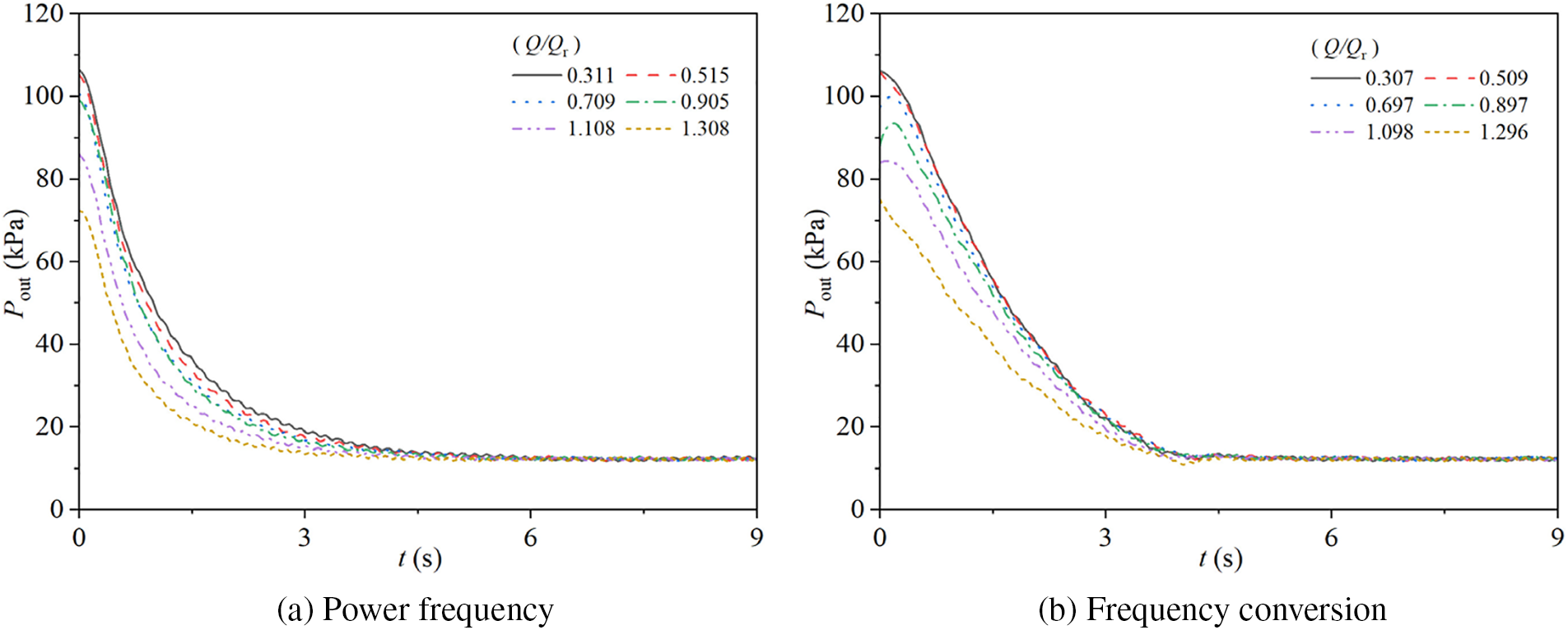
Figure 11: Outlet pressure characteristics for two modes

During power frequency stopping, regardless of the steady-state flow rate ratio, the outlet pressure decreases over time until it stabilizes. For all the different steady-state flow rate ratios (Q/Qr = 0.311, 0.515, 0.709, 0.905, 1.108, 1.308), the rate of decrease in outlet pressure is initially fast and then gradually slows down. In the period where t < 1.5 s, the outlet pressure decreases rapidly; after t ≥ 1.5 s, the rate of decrease becomes slower. The outlet pressure ultimately stabilizes at approximately 12.21 kPa at t = 6.08, 5.55, 5.33, 5.52, 5.09, and 4.48 s, respectively. As the steady-state flow rate ratio increases, the time to reach a stable outlet pressure during power frequency stopping gradually decreases.

During frequency conversion stopping, the outlet pressure for all six different steady-state flow rate ratios exhibits a two-stage change: for t < 4 s, the outlet pressure decreases rapidly in a linear fashion, and for t ≥ 4 s, it gradually reaches a stable value. The outlet pressure stabilizes at approximately 12.42 kPa at t = 4.89, 5.02, 4.95, 5.05, 4.86, and 4.78 s, for Q/Qr = 0.307, 0.509, 0.697, 0.897, 1.098, and 1.296, respectively.

During power frequency stopping, the time it takes for the pump’s outlet pressure to reach a stable value decreases as the steady-state flow rate ratio increases, with the rate of decrease in outlet pressure transitioning from fast to slow before smoothly approaching the stable value; in contrast, during frequency conversion stopping, the time to reach a stable outlet pressure does not significantly change with an increase in the steady-state flow rate ratio. Before reaching the stable value, the rate of decrease in outlet pressure shows minimal variation across different steady-state flow rate ratios, and this rate of decrease gradually slows down as the steady-state flow rate ratio increases, with all ratios ultimately stabilizing at approximately the same time.

Fig. 12 illustrates the variations in pump head during stopping in two different modes. Specifically, Fig. 12a shows the head changes for the pump operating at a power frequency mode with steady-state flow rate ratios of Q/Qr = 0.311, 0.515, 0.709, 0.905, 1.108, and 1.308, while Fig. 12b presents the corresponding head changes for the pump operating at a frequency conversion mode with steady-state flow rate ratios of Q/Qr = 0.307, 0.509, 0.697, 0.897, 1.098, and 1.296.

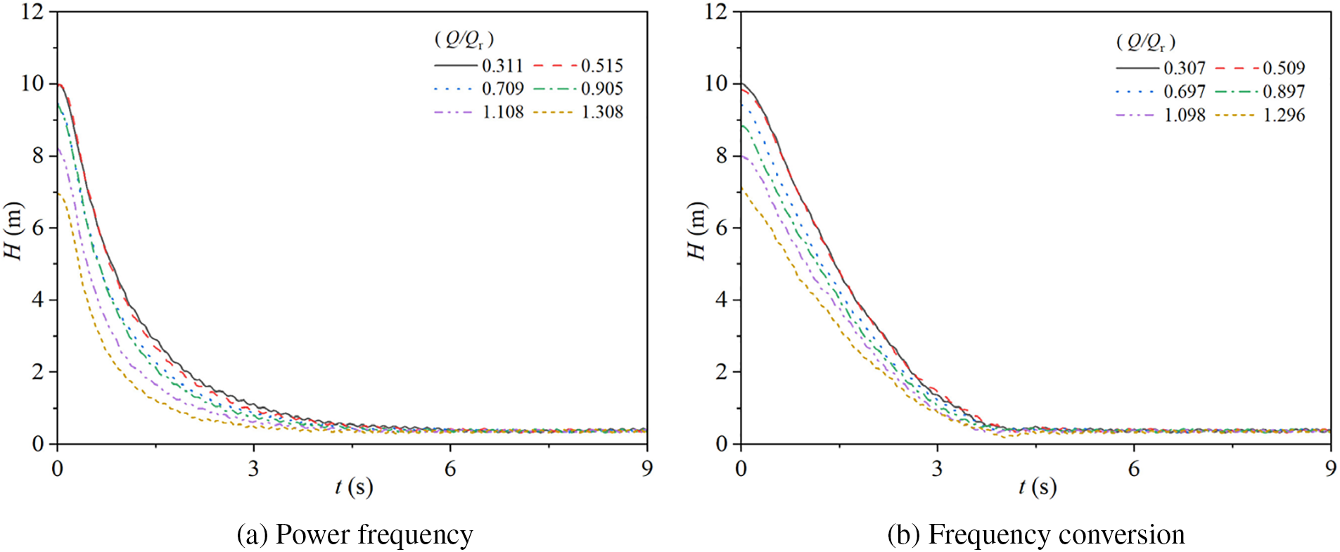
Figure 12: Head characteristics for two modes

In both modes, the pump head exhibits an initial decline followed by stabilization upon stopping. Due to the residual pressure within the pipeline when the pump is turned off, the head does not drop to zero but stabilizes at a low, non-zero value. During power frequency stopping, the head curves for all six steady-state flow rate ratios initially decrease rapidly, followed by a gradual decline until stabilization: for t < 1.5 s, the head decreases quickly, and for t ≥ 1.5 s, the rate of decrease becomes slower, eventually reaching stable values of approximately 0.35 m at t = 6.19, 5.74, 5.42, 5.36, 4.91, and 4.06 s, respectively. The time to reach a stable head value decreases as the steady-state flow rate ratio increases, and before stabilization, the rate of decrease in head transitions from rapid to gradual.

During frequency conversion stopping, the head curves, regardless of the valve opening, exhibit a two-phase characteristic: from 0 s to 4 s, the head decreases rapidly with time, and after t > 4 s, it gradually approaches a stable value. The head for the different steady-state flow rate ratios (Q/Qr = 0.307, 0.509, 0.697, 0.897, 1.098, 1.296) reaches stable values of approximately 0.33 m at t = 4.89, 5.13, 4.64, 4.70, 4.73, and 4.70 s, respectively. The time to reach a stable head value does not significantly change with an increase in the steady-state flow rate ratio, and before stabilization, the rate of decrease in head shows minimal variation across different ratios, with the rate of decrease also slowing down as the steady-state flow rate ratio increases.

Fig. 13 illustrates the variations in flow rate of the experimental pump during stopping in two different modes. Specifically, Fig. 13a shows the flow rate changes for the pump operating at a power frequency mode with steady-state flow rate ratios of Q/Qr = 0.311, 0.515, 0.709, 0.905, 1.108, and 1.308, while Fig. 13b presents the corresponding flow rate changes for the pump operating at a frequency conversion mode with steady-state flow rate ratios of Q/Qr = 0.307, 0.509, 0.697, 0.897, 1.098, and 1.296.

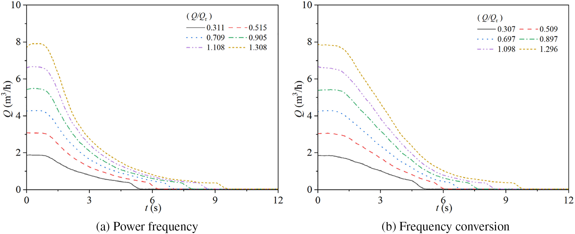
Figure 13: Flow rate characteristics for two modes

In both modes, the flow rate of the pump during stopping exhibits a four-stage pattern: in the first stage, the power frequency mode maintains stable flow rates of 1.88, 3.07, 4.29, 5.49, 6.66, and 7.91 m3/h, respectively, for increasing steady-state flow rate ratios, while the frequency conversion mode maintains stable flow rates of 1.84, 3.06, 4.28, 5.41, 6.60, and 7.85 m3/h, respectively. In the second stage, all six steady-state flow rate ratios in the power frequency mode enter this phase at approximately t = 0.9 s, where the flow rate gradually decreases over time with the rate of decrease transitioning from fast to slow, reaching approximately 0.32 m3/h at t = 4.91, 5.83, 6.61, 7.41, 8.20, and 9.06 s, respectively; in the frequency conversion mode, the flow rates enter this phase at approximately t = 1.1 s, reaching approximately 0.35 m3/h at t = 4.58, 5.58, 6.31, 7.22, 8.09, and 9.41 s, respectively. In the third stage, both starting modes experience a sudden change in the rate of decline, with the power frequency mode’s flow rates rapidly decreasing from 0.32 to 0 m3/h at t = 5.45, 6.36, 7.22, 8.02, 8.73, and 9.64 s, respectively, and the frequency conversion mode’s flow rates rapidly decreasing from 0.35 to 0 m3/h at t = 5.19, 6.16, 6.92, 7.77, 8.59, and 9.89 s, respectively. As the steady-state flow rate ratio increases, the stable flow rate before pump stopping also increases, and consequently, the time required for the flow rate to decrease to 0 m3/h upon completion of the stopping process gradually increases.

Fig. 14 illustrates the changes in rotational speed of the experimental pump during stopping in two different modes. Specifically, Fig. 14a shows the speed changes for the pump operating at a power frequency mode with steady-state flow rate ratios of Q/Qr = 0.311, 0.515, 0.709, 0.905, 1.108, and 1.308, while Fig. 14b presents the corresponding speed changes for the pump operating at a frequency conversion mode with steady-state flow rate ratios of Q/Qr = 0.307, 0.509, 0.697, 0.897, 1.098, and 1.296.

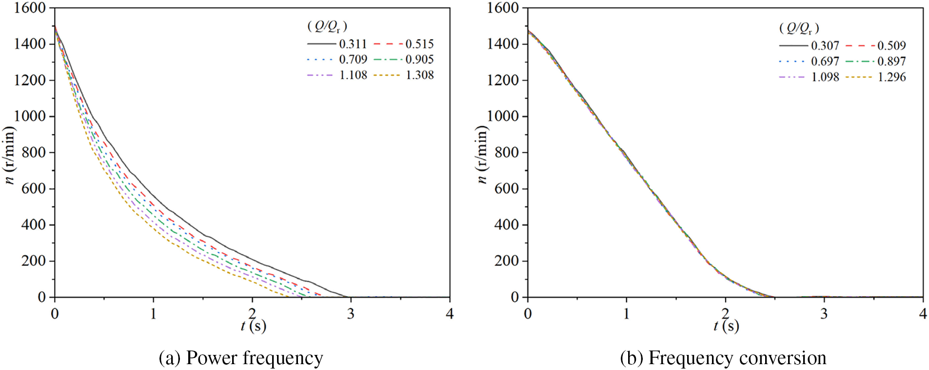
Figure 14: Rotational speed characteristics for two modes

In the power frequency mode, the pump’s rotational speed decreases from 1470 rpm to 0 as time progresses. The rate of decrease in speed slows down over time; it is faster in the 0 s to 1 s interval and slower after t > 1 s. The six steady-state flow rate ratios reach 0 rpm at t = 2.97, 2.77, 2.70, 2.63, 2.52, and 2.39 s, respectively. As the steady-state flow rate ratio increases, the time required for the speed to decrease to 0 gradually decreases.

In the frequency conversion mode, the pump’s rotational speed also decreases with time for all six steady-state flow rate ratios. For t < 1.9 s, the speed decreases linearly, and for t ≥ 1.9 s, the rate of decrease gradually slows down, with all ratios reaching 0 rpm at approximately t = 2.48 s. The change in steady-state flow rate ratio does not significantly affect the speed curves during stopping.

During stopping, the time for the pump’s speed to decrease to 0 in the power frequency mode decreases as the steady-state flow rate ratio increases, whereas there is no significant difference in the frequency conversion mode. In the tested six steady-state flow rate ratios, the time for the pump’s speed to decrease to 0 in the power frequency mode is consistently longer than in the frequency conversion mode.

Fig. 15 illustrates the changes in torque of the experimental pump during stopping in two different modes. Specifically, Fig. 15a shows the torque changes for the pump operating at a power frequency mode with steady-state flow rate ratios of Q/Qr = 0.311, 0.515, 0.709, 0.905, 1.108, and 1.308, while Fig. 15b presents the corresponding torque changes for the pump operating at a frequency conversion mode with steady-state flow rate ratios of Q/Qr = 0.307, 0.509, 0.697, 0.897, 1.098, and 1.296.

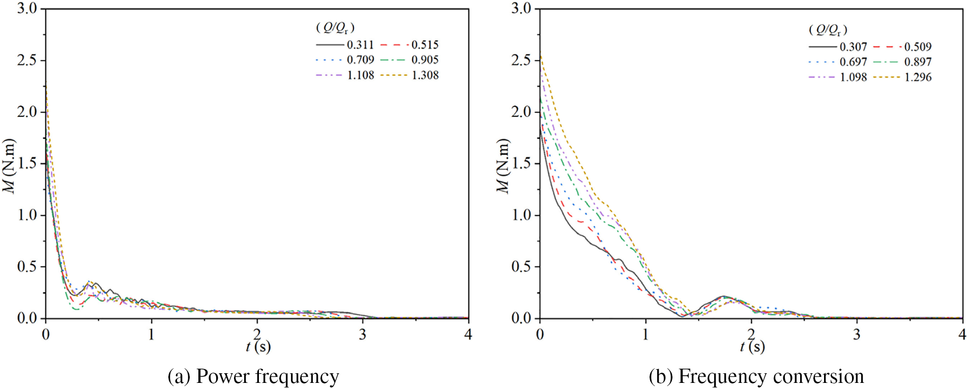
Figure 15: Torque characteristics for two modes

In the power frequency mode, the torque for all six steady-state flow rate ratios initially decreases rapidly. The torque reaches its minimum values at t = 0.27, 0.30, 0.31, 0.31, 0.31, and 0.30 s, with values of 0.23, 0.14, 0.29, 0.09, 0.23, and 0.22 N·m, respectively. After reaching these minima, the torque briefly increases, reaching 0.34, 0.22, 0.36, 0.22, 0.33, and 0.36 N·m at t = 0.47, 0.42, 0.41, 0.47, 0.41, and 0.41 s, respectively. Subsequently, the torque decreases slowly over time. In the 0.5 to 1.5 s interval, the torque exhibits larger fluctuations, and from 1.5 to 2.5 s, it decreases more smoothly, ultimately reaching 0 at t = 3.36, 2.94, 2.86, 2.75, 2.64, and 2.61 s, respectively. As the steady-state flow rate ratio increases, the time required for the torque to reach 0 gradually decreases.

In the frequency conversion mode, the torque for all six steady-state flow rate ratios also initially decreases rapidly, reaches a minimum, briefly increases, and then gradually decreases to 0. From 0 to 1.5 s, the torque decreases quickly, with the initial values of 1.86, 2.00, 2.03, 2.15, 2.44, and 2.60 N·m, decreasing to minima of 0.02, 0.03, 0.02, 0.02, 0.03, and 0.05 N·m at t = 1.36, 1.38, 1.34, 1.44, 1.44, and 1.56 s, respectively. From 1.5 to 1.8 s, the torque briefly increases, reaching 0.22, 0.21, 0.21, 0.20, 0.16, and 0.16 N·m at t = 1.75, 1.77, 1.73, 1.80, 1.82, and 1.85 s, respectively. After this, the torque continues to decrease until it reaches 0: from 1.8 to 2 s, the torque decreases; from 2 to 2.4 s, the torque decreases very slowly; and from 2.4 to 2.6 s, the torque decreases again, ultimately reaching 0 at t = 2.61, 2.67, 2.61, 2.64, 2.63, and 2.59 s, respectively. As the steady-state flow rate ratio increases, the times to reach the minimum and maximum torque values are slightly delayed, but all ratios eventually reach 0 at approximately the same time.

Compared to the power frequency mode, the time required for the torque to decrease to 0 in the frequency conversion mode is shorter. However, in the fluctuation phase before the torque reaches 0, the times to reach the minimum and subsequent peak torque values in the frequency conversion mode are slightly delayed compared to the power frequency mode. The torque curves in the frequency conversion mode show significant differences with varying steady-state flow rate ratios, whereas the torque curves in the power frequency mode do not exhibit substantial variations across the tested six steady-state flow rate ratios.

Fig. 16 illustrates the changes in shaft power of the experimental pump during stopping in two different modes. Specifically, Fig. 16a shows the shaft power changes for the pump operating at a power frequency mode with steady-state flow rate ratios of Q/Qr = 0.311, 0.515, 0.709, 0.905, 1.108, and 1.308, while Fig. 16b presents the corresponding shaft power changes for the pump operating at a frequency conversion mode with steady-state flow rate ratios of Q/Qr = 0.307, 0.509, 0.697, 0.897, 1.098, and 1.296.

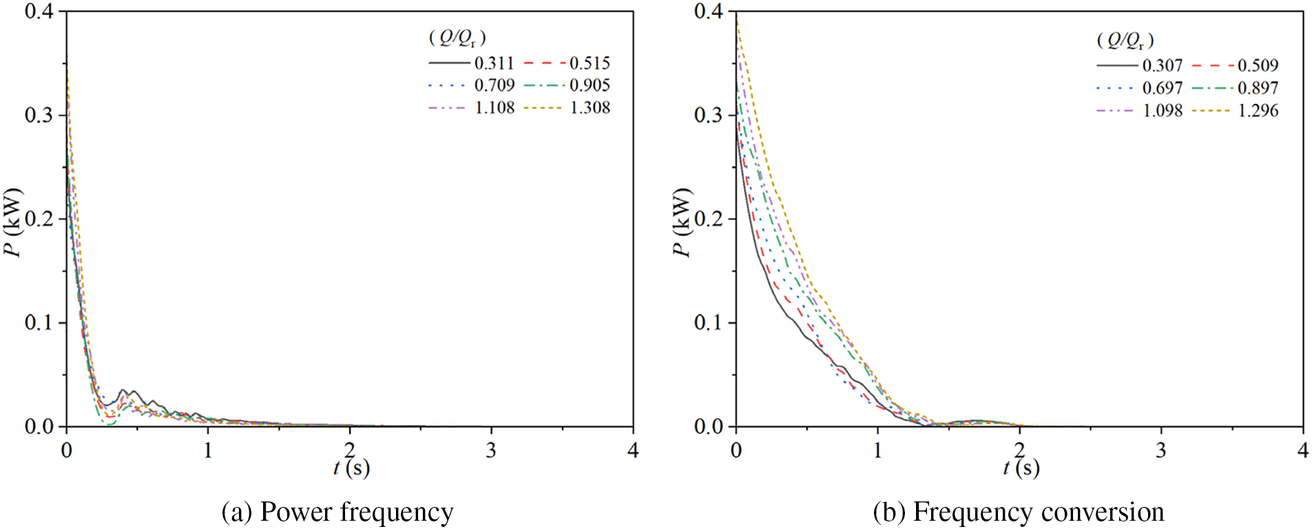
Figure 16: Shaft power characteristics for two modes

In the power frequency mode, the shaft power initially decreases rapidly, reaches a minimum, briefly increases, and then gradually decreases to 0. During the 0 s to 0.3 s interval, the shaft power for the steady-state flow rate ratios of Q/Qr = 0.311, 0.515, 0.709, 0.905, 1.108, and 1.308 decreases quickly from initial values of 0.26, 0.27, 0.23, 0.28, 0.34, and 0.36 kW, respectively, to minima of 0.02, 0.01, 0.02, 0.01, 0.02, and 0.01 kW at t = 0.30 s. After reaching these minima, the shaft power briefly increases, reaching 0.04, 0.02, 0.04, 0.02, 0.03, and 0.03 kW at t = 0.39, 0.42, 0.41, 0.47, 0.41, and 0.44 s, respectively. Finally, the shaft power decreases slowly, reaching 0 at t = 1.84, 1.64, 1.70, 1.56, 1.52, and 1.42 s, respectively.

In the frequency conversion mode, the shaft power for all six steady-state flow rate ratios also initially decreases rapidly, reaches a minimum, slightly increases, and then decreases to 0. During the 0 s to 1.3 s interval, the shaft power decreases quickly from initial values of 0.29, 0.31, 0.31, 0.33, 0.38, and 0.40 kW, respectively, to minima of 0 kW at t = 1.33, 1.34, 1.37, 1.44, 1.44, and 1.41 s, respectively. After reaching these minima, the shaft power briefly increases, reaching 0.01 kW at t = 1.72 s, and finally decreases to 0 at approximately t = 2.03 s for all ratios.

Compared to the power frequency mode, the initial shaft power values in the frequency conversion mode are higher, and the time required for the shaft power to decrease to 0 is longer. The shaft power curves in the frequency conversion mode show more significant differences with varying steady-state flow rate ratios, whereas the shaft power curves in the power frequency mode exhibit smaller variations as the steady-state flow rate ratio increases.

4  Performance Prediction

This paper employs eight machine learning models to fit the external characteristics of the pump and investigates the reliability of predictions made by these models. The models are as follows: M1 is Support Vector Machine Regression (SVMR) [27], M2 is Gaussian Process Regression (GPR) [28], M3 is Decision Tree Regression (DTR) [29], M4 is an ensemble regression model combining Gradient Boosting Trees Regression (GBTR) and Random Forests Regression (RFR) [29], M5 is K-Nearest Neighbors Regression (KNNR) [29], M6 is a Feedforward Neural Network (FNN) [30], M7 is a Deep Learning Network (DLN) [31], and M8 is a Generalized Additive Model (GAM) [32]. These eight machine learning models are used to predict the external characteristic curves of the pump in both power frequency and frequency conversion modes.

The training dataset consists of sample points from five external characteristic curves, corresponding to the expected steady-state flow rate ratios Q/Qr = 0.30, 0.50, 0.70, 0.90, and 1.10. The test dataset includes the inlet pressure, outlet pressure, head, flow rate, rotational speed, torque, and shaft power at the expected steady-state flow rate ratio Q/Qr = 1.3 during the starting and stopping periods for both power frequency and frequency conversion modes. The accuracy of the prediction results is evaluated using the absolute error and relative error between the predicted values and the experimental data, with the formulas for absolute error (Eq. (1)) and relative error (Eq. (2)) as follows:

Δ=X1−X (1)

δ=X1−XX (2)

In the above two formulas, Δ represents the absolute error value, δ represents the relative error value, X1 is the predicted value, and X is the experimental value. The final criteria for evaluating the prediction accuracy are obtained by calculating the average of the absolute values of the relative errors and the average of the absolute values of the absolute errors over the entire prediction curve.

4.1 Prediction Model

The objective of the Support Vector Regression (SVR) model is to identify a function that optimally fits the data while maintaining a specified tolerance for error. Unlike traditional least squares methods, SVR enhances the generalization capability of the model by seeking a flat function. To address nonlinear relationships, SVR employs various kernel functions to map the original feature space into a higher-dimensional space, thereby facilitating the identification of a separating hyperplane. For nonlinear models, the input data is first mapped into a feature space using a kernel function, after which regression is performed. The underlying principle is illustrated in Fig. 17, and the mathematical formulation is provided in Eqs. (3) through (6).

minw,b,ξi,ξ^i12wTw+C∑i=1m(ξi+ξ^i) (3)

s.t. f(xi)−yi≤ε+ξi (4)

yi−f(xi)≤ε+ξ^i (5)

ξi≥0,ξ^i≥0,i=1,2,⋯,m (6)

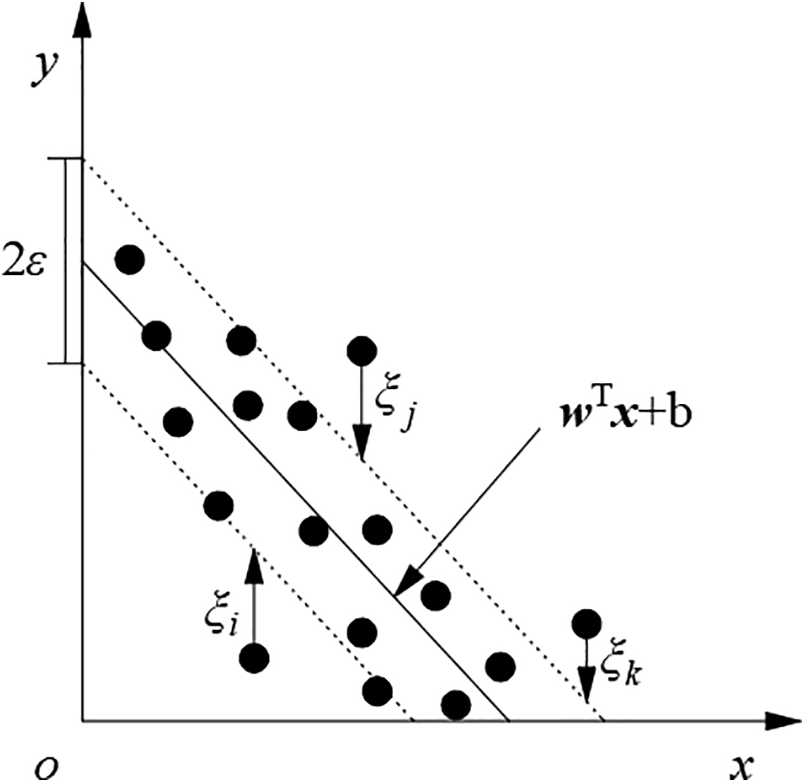
Figure 17: Principle of support vector regression

In the equations, w and b are the parameters to be determined by the model; xi represents the feature values of the sample; yi is the target value of the sample; C is the penalty coefficient; ξi is the slack variable; and ε is the margin of tolerance, representing the maximum deviation allowed between the predicted value f(xi) and the actual value yi without incurring a penalty.

In the Gaussian Process Regression (GPR), a Gaussian Process reflects the empirical risk through a Gaussian likelihood function, ensuring that any finite number of random variables follows a joint Gaussian distribution. Given a training dataset D = {(xi, yi) | i = 1, ..., n} where xi is a d-dimensional input vector and yi is the corresponding target variable [34], the Gaussian Process Regression (GPR) model assumes that the prior distribution of the target variables is Gaussian. The model is defined by a mean function m(x) and a covariance function k(x, x′):

m(x)=E(f(x))k(x,x′)=E[(f(x)−m(x))(f(x′)−m(x′))]} (7)

Following the Bayesian principle, the prediction for a test set sample y* is assumed to follow a Gaussian distribution. The estimated mean y¯∗ and variance cov(y*) of y* are given by:

y¯∗=k(x∗,x)[k(x,x)+σn2In]−1y (8)

cov(y∗)=k(x∗,x∗)−k(x∗,x)[k(x,x)+σn2In]−1k(x,x∗) (9)

The covariance function, often referred to as the kernel function, is central to GPR and determines the shape of both the prior and posterior distributions. The kernel function encodes the “similarity” between data points, which in turn influences the smoothness and structure of the functions drawn from the Gaussian process. There are various types of kernel functions, each with its own method of measuring similarity, leading to different shapes of the resulting Gaussian process models and probability distributions. In this paper, the most common Radial Basis Function (RBF) kernel, also known as the Gaussian or squared exponential kernel, is chosen to construct the GPR model. The mathematical expression for the RBF kernel is given by:

k(xi,xj)=exp⁡(−d(xi,xj)22l2) (10)

Decision trees are a type of supervised learning method and serve as a tree-like classifier, consisting primarily of leaf nodes, a root node, and internal nodes. The root node is unique and serves as the starting point for the training and prediction process. Data is progressively split based on the feature attributes at each non-leaf node, creating multiple sub-datasets that are then passed to the next level of nodes. The splitting process continues until the data reaches the leaf nodes, at which point no further splits occur. The data in the leaf nodes is then processed to produce the final prediction. For each sub-dataset S[i] a decision tree is constructed, and with n bootstrap sub-datasets, a total of n decision trees are built [35]. The construction steps for each tree are as follows:

(1) Select the optimal feature value for node splitting. Among all possible values of each feature in the exhaustive subspace, choose the split point that minimizes the mean squared error (MSE). The mean squared error is calculated as follows:

MSE=1l∑i=1l(yi−y^i)2 (11)

In the equation: l is the number of samples in the subspace; yi is the true output for the i-th sample; y^i is the estimated output for the i-th sample as predicted by the decision tree.

(2) On the basis of the node splitting, the optimal split points are selected for further splitting on the resulting child nodes. The selection of the optimal split points is based on the criterion of minimizing the mean squared error.

(3) The splitting process as described in step (2) is repeated until the stopping criteria are met.

Ultimately, the n decision trees each provide a prediction for the input sample. The n predictions are denoted as {x1, x2, ..., xn}, where xi, with i ϵ {1, 2, ..., n}, represents the predicted remaining useful life of the engine by the i-th decision tree.

Ensemble regression models integrate the predictions from multiple regression models to make a final decision. These models are built in a specific sequence, and there is a dependency relationship between them. In this study, an ensemble regression model is constructed using Gradient Boosting Trees Regression (GBTR) and Random Forest Regression (RFR).

GBTR generates a strong learner by combining a set of weak learners. The core idea is to add new regression trees that minimize the objective function at each iteration. Each new tree is trained on the residuals of the previous tree, and the training is performed in the direction of the negative gradient of the loss function. Through multiple iterations, the weak learners are linearly combined to form a strong learner [29]. The algorithm for the GBTR model is as follows:

Initialize the decision tree:

f0(x)=argmin∑i=1nL(yi,c) (12)

Compute the negative gradient of the loss function with respect to the current model as an estimate of the residuals:

rmh=−[∂L(yh,f(xh))∂f(xh)]f(x)=fm−1(x) (13)

Fit a regression tree to get the leaf node regions Rmj for the m-th tree, where j = 1, 2, ..., J represents the number of nodes in each tree. For each j, use a line search to estimate the value of the leaf node region that minimizes the loss function, and calculate the optimal fitted value:

cmj(x)=argmin∑xh∈RmjL(yi,fm−1(xi)+c) (14)

Update to the strong learner:

fm(x)=fm−1(x)+∑j=1JcmjI,x∈Rmj (15)

Obtain the final regression tree by summing the values of the leaf nodes from each tree:

F(x)=∑m=1M∑j=1JcjmI,x∈Rmj (16)

Random Forest Regression (RFR) can be mathematically summarized as follows: Given a dataset X and a set of predictions Y, a forest that depends on the random variable θ is grown, forming tree predictors h(x, θk), where the output of each predictor is a numerical value. The Random Forest predictor is obtained by averaging the predictions of these trees {h(x, θk)} over k [36]. A training set is composed of samples drawn independently from the distribution of the random variables Y and X. The mean squared generalization error for any tree predictor h(X) is given by EX,Y(Y-h(X))2. As the number of trees in the forest approaches infinity, the following holds everywhere:

EX,Y(Y−avkh(X,θk))2→EX,Y(Y−Eθh(X,θ))2 (17)

Thus, the Random Forest regression function is: Y = Eθh(X, θ). In practice, when using a sufficiently large number of trees, the approximation is used: Y = avkh(X, θk). The error analysis is as follows:

PE∗(tree)=EθEX,Y(Y−h(X,θ))2 (18)

where PE* represents the average generalization error of the Random Forest.

K-Nearest Neighbors Regression (KNNR) is an instance-based learning method that makes predictions by finding the closest training data points to a given test point. This method is simple and intuitive, suitable for continuous value prediction problems. Given a new observation, the KNNR model identifies the k nearest neighbors (based on Euclidean distance) and predicts the output for the new point based on the outputs of these k neighbors [37].

In regression prediction, assume there is a set S = {(x1,y1),(x2,y2),...,(xn,yn)} containing n sample points, where xi (i = 1, ..., n) are points in an N-dimensional Euclidean space, and yi (i = 1, …, n) are the corresponding values. The k nearest sample points to the new point can be selected, and a weighted average of their y-values can be taken to obtain the y-value for the new point. This can be expressed mathematically as:

y=∑(xiyi)∈Nk(x)ωiyi (19)

Nk(x) is the set of the k nearest points to the sample point x; ωi is the weight associated with the i-th nearest neighbor.

Feedforward Neural Network (FNN) in Fig. 18 is adept at modeling complex nonlinear relationships and are a typical type of neural network model, also known as multilayer perceptrons. A FNN consists of an input layer, one or more hidden layers, and an output layer. The input layer receives the raw data, the hidden layers perform transformations and feature extraction on the input data, and the output layer produces the model’s predictions based on the results from the hidden layers [38]. Each layer is composed of several neurons, and the weights of each neuron are iteratively optimized using the backpropagation algorithm.

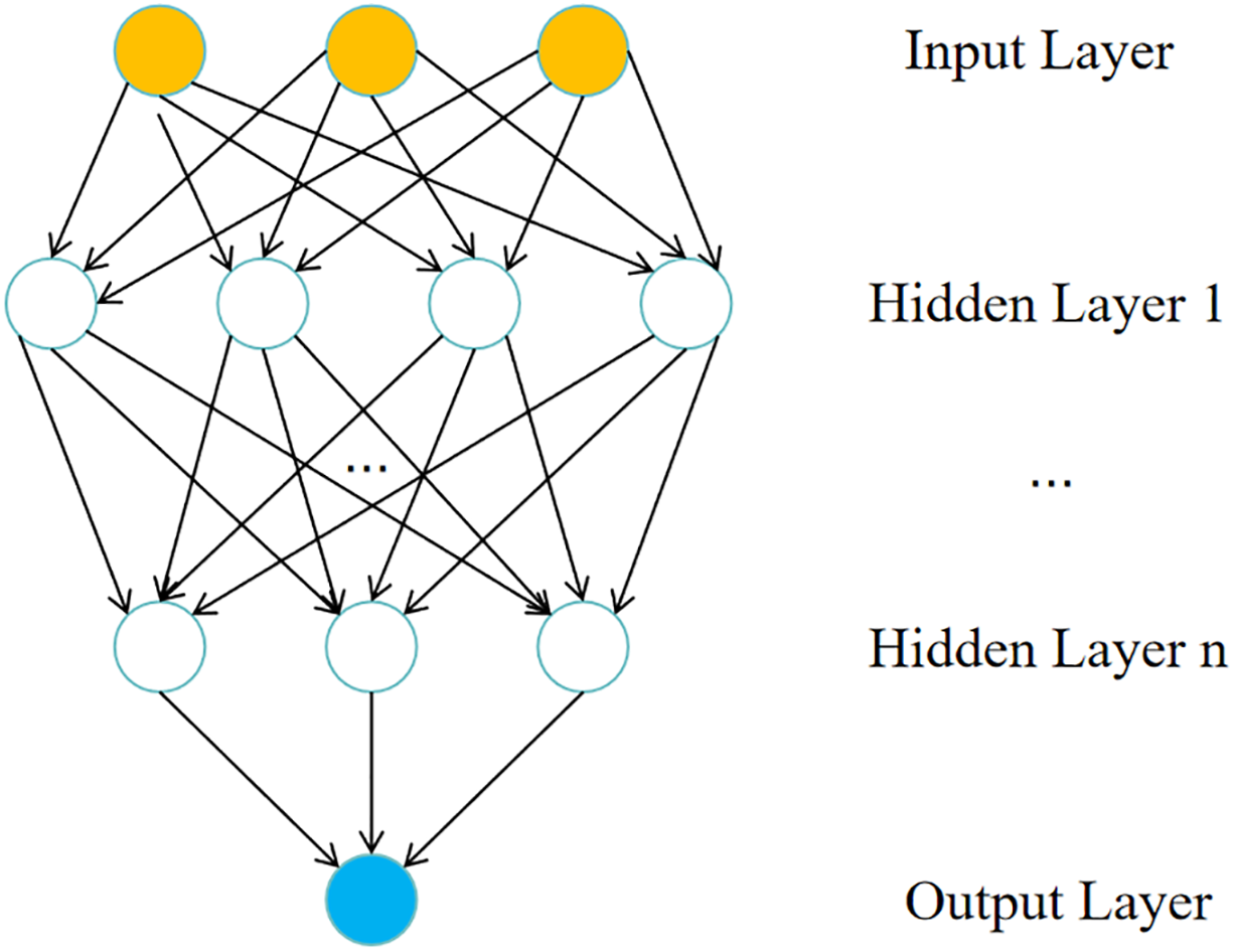
Figure 18: Feedforward neural network

Feedforward Neural Networks propagate information through the network using the following equations:

z(l)=W(l)⋅a(l−1)+b(l),a(l)=fl(z(l)) (20)

Through layer-by-layer information propagation, the final output a(l) of the network is obtained, where l represents the layer index, fl is the activation function for the neurons in layer l, W(l) is the weight matrix from layer l−1 to layer l, b(l) is the bias from layer l−1 to layer l, z(l) is the net input to the neurons in layer l, and a(l) is the output of the neurons in layer l. The entire network can be viewed as a composite function, with vector x as the input to the first layer a(0), and the output of layer l a(l) as the output of the function.

Compared to FNN, Deep Learning Network (DLN) have many more hidden layers (typically tens or even hundreds of layers), which allows them to learn more complex hierarchical feature representations [33]. Due to their multi-layered architecture, DLN are capable of handling more complex datasets, such as those in image recognition, speech recognition, and natural language processing. In these domains, they often outperform shallower networks.

Generalized Additive Models (GAM) combine the Generalized Linear Model (GLM) and additive models to achieve higher accuracy than simple models while retaining the good interpretability of linear models [32]. The general form is:

y=f1(x1)+f2(x2)+⋯+fn(xn)+ε (21)

y is the dependent variable; xi is the i-th feature variable, with i = 1, 2, ..., n, and n is the total number of features; ε is the error term, which follows a normal distribution ε ~(0, σ2) and is independent of the features; fi( xi) is a nonlinear function related to the i-th feature, most commonly composed of a sum of B-spline basis functions, which can quantify the relationship between the feature xi and the dependent variable y.

The form of fi( xi) is:

fi(xi)=∑j=1kiβi,jbi,j(xi) (22)

bi,j( xi) is the j-th B-spline basis of fi( xi), with the most common being the cubic B-spline basis. According to the properties of B-splines, a q-degree B-spline basis is composed of q + 1 polynomials of degree q determined by q + 2 knots; βi,j is the weight for the j-th B-spline basis; ki is the number of spline bases, which is a parameter of the model.

4.2 Power Frequency Starting Mode Performance Prediction

Fig. 19 illustrates the prediction of seven external characteristic curves for the experimental pump at a steady-state flow rate ratio of Q/Qr = 1.308 during starting in power frequency mode. In Fig. 19a, five inlet pressure prediction models are presented. The M2 to M5 curves exhibit a consistent pattern with the experimental data, characterized by an initial rapid decrease to a trough followed by a rapid increase before reaching a stable value. Conversely, the M8 curve shows a gradual decline followed by a gradual rise without a significant dip before stabilization. The stable values of all five methods are slightly higher than the experimental data. Prior to stabilization, the trough of the M2 curve is significantly higher than the experimental data, and the trough of the M8 curve is also higher, with average absolute errors of 0.0015 and 0.0027 kPa, and average relative errors of 36.59% and 75.12%, respectively. The M3, M4, and M5 curves, however, show closer troughs and overall shapes to the experimental data, with average absolute errors of 0.0005, 0.0013, and 0.0012 kPa, and average relative errors of 37.24%, 37.21%, and 34.73%, respectively. The M1, M6, and M7 curves have been omitted from the figure due to unsatisfactory prediction results. Based on the average relative and absolute errors, the M2 to M5 models demonstrate satisfactory predictive performance, with the M3 model (DTR) showing the best predictive accuracy.

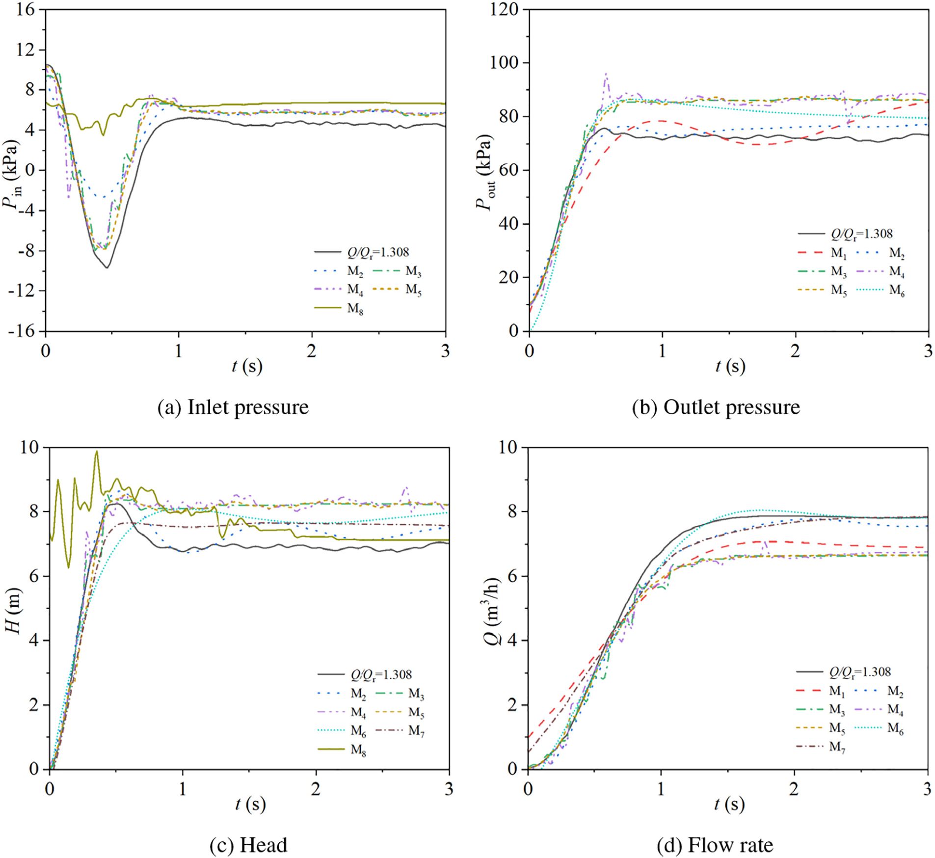
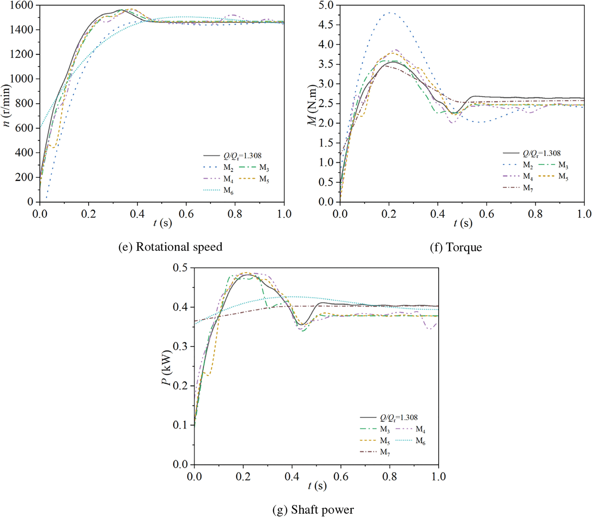
Figure 19: Power frequency starting mode external characteristics prediction

In Fig. 19b, six outlet pressure prediction models are presented. All six models show a rapid initial increase followed by stabilization. Specifically, the M1 curve exhibits significant fluctuations around the stable value of the experimental data after t > 0.5 s, with an average absolute error of 0.0054 kPa and an average relative error of 7.82%. The M2 curve closely matches the experimental data before and after reaching the stable value, with an average absolute error of 0.0051 kPa and an average relative error of 7.41%. The M3 to M5 curves also align well with the experimental data before stabilization, but their stable values are higher than the experimental data, with average absolute errors of 0.0130, 0.0131, and 0.0130 kPa, and average relative errors of 18.06%, 18.45%, and 18.22%, respectively. The M6 curve gradually approaches the stable value of the experimental data after reaching its maximum, with an average absolute error of 0.0077 kPa and an average relative error of 12.36%. The M7 and M8 curves have been omitted from the figure due to unsatisfactory prediction results. Based on the average relative and absolute errors, the M2 model (GPR) demonstrates the best predictive performance.

In Fig. 19c, seven head prediction models are displayed. The M2 to M7 curves show a high degree of agreement with the experimental data before reaching their maximum values. After reaching the maximum, the M2 curve follows the trend of the experimental data, initially decreasing and then fluctuating around the stable value of the experimental curve, with an average absolute error of 0.54 m and an average relative error of 7.84%. The M3 to M7 curves stabilize after reaching their maximum values, all showing higher stable values than the experimental data, with average absolute errors of 1.21, 1.23, 1.22, 0.98, and 0.67 m, and average relative errors of 14.54%, 14.79%, 16.86%, 8.24%, and 2.22%, respectively. The M8 curve exhibits significant discrepancies during the rapid increase phase of the experimental data, showing an oscillatory trend, but it gradually decreases and approaches the stable value of the experimental curve, with an average absolute error of 0.91 m and an average relative error of 121.74%. The M1 curve is omitted from the figure due to unsatisfactory prediction results. Based on the average relative and absolute errors, the M2, M6, and M7 models demonstrate better predictive performance, with the M7 model (DLN) showing the best predictive accuracy.

In Fig. 19d, seven flow rate prediction models are presented, all of which exhibit a trend of rapid initial increase followed by stabilization, consistent with the experimental curve. The M1 curve shows higher flow rates than the experimental data during the initial rise (0–0.6 s), after which it becomes lower, and its stable value is below that of the experimental curve, with an average absolute error of 0.89 m3/h and an average relative error of 47.54%. The M2 and M6 curves show good overall agreement with the experimental data, with average absolute errors of 0.21 and 0.10 m3/h, and average relative errors of 13.57% and 16.71%, respectively. The M3, M4, and M5 curves align well with the experimental data from 0 to 0.7 s, but they stabilize at values lower than the experimental curve’s stable value after 0.7 s, with average absolute errors of 1.04, 1.03, and 1.02 m3/h, and average relative errors of 15.05%, 16.59%, and 13.73%, respectively. The M7 curve has a slightly slower increase in flow rate compared to the experimental data from 0 to 1.3 s, but it gradually approaches and matches the stable value of the experimental curve, with an average absolute error of 0.22 m3/h and an average relative error of 24.81%. The M8 curve is omitted from the figure due to unsatisfactory prediction results. Based on the average relative and absolute errors, the M2, M6, and M7 models demonstrate better predictive performance, with the M6 model (FNN) showing the best predictive accuracy.

In Fig. 19e, five rotational speed prediction models are displayed. All five models exhibit a rapid initial increase followed by stabilization, consistent with the experimental curve. Specifically, the M2 curve shows slightly lower rotational speeds than the experimental data during the rapid increase phase (0–0.3 s), but it gradually approaches and maintains high agreement with the stable value of the experimental curve, with an average absolute error of 21.72 r/min and an average relative error of 2.97%. The M3 curve shows a high degree of agreement with the experimental data throughout, with an average absolute error of 8.69 r/min and an average relative error of 0.83%. The M4 curve is also in good agreement with the experimental data, although it exhibits minor fluctuations in the middle, with an average absolute error of 10.01 r/min and an average relative error of 0.81%. The M5 curve closely matches the experimental data from 0 to 0.3 s, with small fluctuations, and stabilizes at around t = 0.45 s, aligning with the stable value of the experimental curve, with an average absolute error of 8.24 r/min and an average relative error of 0.89%. The M6 curve starts with a significantly higher initial rotational speed than the experimental data and increases more slowly from 0 to 0.3 s, but it aligns well with the experimental data in the stable phase, with an average absolute error of 18.03 r/min and an average relative error of 2.32%. The M1, M7, and M8 curves are omitted from the figure due to unsatisfactory prediction results. Based on the average relative and absolute errors, the M3, M4, and M5 models demonstrate better predictive performance, with the M5 model (KNNR) showing the best predictive accuracy.

In Fig. 19f, five torque prediction models are presented, all of which show a trend of initially rapid increase, followed by a decrease, and finally stabilization, consistent with the experimental curve. Specifically, the M2 curve exhibits a peak value significantly higher than that of the experimental curve, reaches the stable value later than the experimental curve, and has a slightly lower stable value, with an average absolute error of 0.32 N·m and an average relative error of 12.17%. The M3 to M5 curves show good overall agreement with the experimental data; their peak values are slightly higher, and their stable values are slightly lower than those of the experimental curve, aligning with the time at which the experimental curve reaches its stable value. The average absolute errors for M3, M4, and M5 are 0.18, 0.18, and 0.19 N·m, respectively, and the average relative errors are 6.93%, 7.21%, and 7.36%, respectively. The M7 curve shows significant differences from the experimental curve before reaching the stable value, but its stable value is close to that of the experimental curve, with an average absolute error of 0.04 N·m and an average relative error of 2.27%. The M1, M6, and M8 curves are omitted from the figure due to unsatisfactory prediction results. Based on the average relative and absolute errors, the M3, M4, M5, and M7 models demonstrate better predictive performance, with the M7 model (DLN) showing the best predictive accuracy.

In Fig. 19g, five shaft power prediction models are presented. The M3 to M5 curves show a trend that is consistent with the experimental curve, where the shaft power initially increases rapidly, then decreases, increases again, and finally stabilizes. In contrast, the M6 and M7 curves exhibit a more stable profile overall. Specifically, the M3 curve aligns well with the experimental data during the rapid increase phase but shows significant differences between 0.2 and 0.4 s, and its final stable value is slightly lower than that of the experimental curve, with an average absolute error of 0.0297 kW and an average relative error of 6.53%. The M4 and M5 curves also show good overall agreement with the experimental data, but their stable values are slightly lower, with average absolute errors of 0.0316 kW for both, and average relative errors of 6.70% and 6.46%, respectively. The M6 and M7 curves do not show similar changes to the experimental curve from 0 s to 0.5 s, showing a larger overall discrepancy, but they closely match the stable value of the experimental curve in the stabilization phase, with average absolute errors of 0.0176 and 0.0134 kW, and average relative errors of 2.92% and 2.63%, respectively. The M1, M2, and M8 curves are omitted from the figure due to unsatisfactory prediction results. Based on the average relative and absolute errors, the M2, M6, and M7 models demonstrate better predictive performance, with the M7 model (DLN) showing the best predictive accuracy.

Table 2 presents the mean absolute errors and mean relative errors of the external characteristic curves predicted by each machine learning model compared to the experimental curves during power frequency starting. Some prediction methods that exhibited excessively large average errors for certain external characteristic parameters have been excluded from the table for reference purposes. From the table, it can be observed that Models M3 to M5 achieved relatively high prediction accuracy across all parameters, rendering their results more reliable. In contrast, Models M1, M7, and M8 generally performed poorly in terms of prediction accuracy. Notably, when predicting the inlet pressure, all eight machine learning models exhibited small mean absolute errors but large mean relative errors. This is due to the fact that the experimental values of the inlet pressure fluctuated near zero during the 0–1 s interval, leading to very small denominators in the relative error calculations and thus resulting in larger relative errors. For the prediction of head, Model M8 showed a small mean absolute error but an extremely large mean relative error. This is attributed to the experimental values of head gradually increasing from zero during the 0–0.5 s interval, while the predicted values exhibited significant fluctuations around a higher value starting from 0 s. The near-zero experimental values led to the generation of extremely large relative errors.

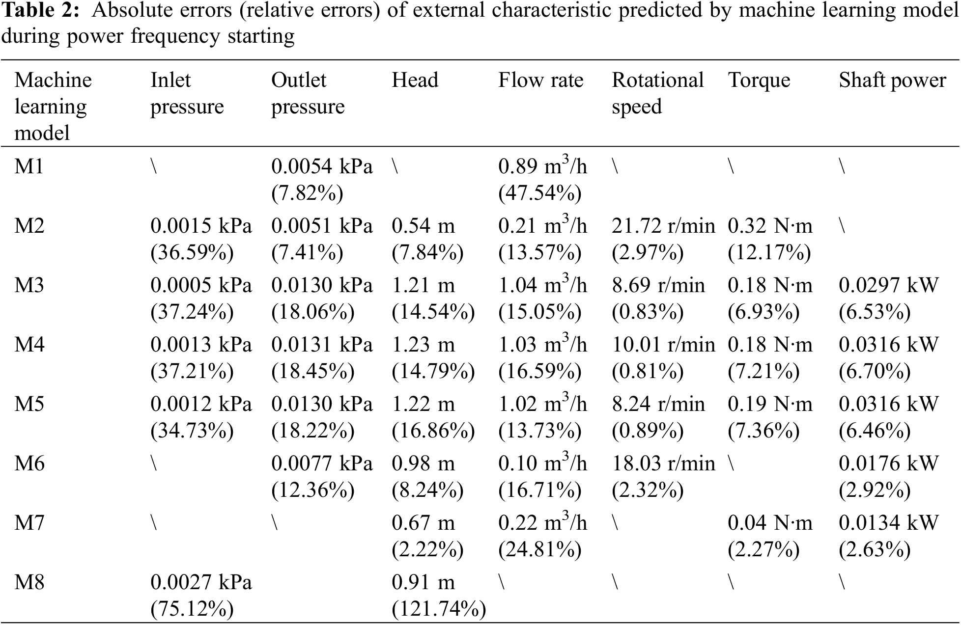
4.3 Power Frequency Stopping Mode Performance Prediction

Fig. 20 illustrates the prediction of seven external characteristic curves for the experimental pump at a steady-state flow rate ratio of Q/Qr = 1.308 during stopping in power frequency mode. In Fig. 20a, eight models predicting the pump’s inlet pressure are presented. The M1 to M5 curves generally follow the trend of the experimental data, showing a rapid increase from 0 to 0.5 s, reaching a maximum value, and then slowly decreasing to a stable value. The M1 curve shows slight differences from the experimental data during the rapid rise phase but aligns well with the experimental curve after t > 3 s, with an average absolute error of 0.0002 kPa and an average relative error of 2.67%. The M2 to M5 curves show high agreement with the experimental data, with average absolute errors of 0.0002, 0.0001, 0.0001, and 0.0001 kPa, and average relative errors of 2.37%, 1.24%, 1.30%, and 0.98%, respectively. The M6 curve exhibits significant differences from the experimental data from 0 s to 3 s, starting from an initial value of 8.09 kPa and rising slowly, reaching a maximum value, and then gradually decreasing to a stable value that is slightly lower than the experimental curve’s stable value, with an average absolute error of 0.0004 kPa and an average relative error of 5.39%. The M7 curve shows large discrepancies from the experimental data throughout and never reaches a stable state, with an average absolute error of 0.0009 kPa and an average relative error of 10.55%. The M8 curve initially decreases rapidly and then increases rapidly within the 0 s to 1 s interval, showing significant differences from the experimental data, and its stable value is slightly lower than the experimental curve, with an average absolute error of 0.0007 kPa and an average relative error of 8.54%. Based on the average relative and absolute errors, the M2 to M5 models demonstrate better predictive performance, with the M5 model (KNNR) showing the best predictive accuracy.

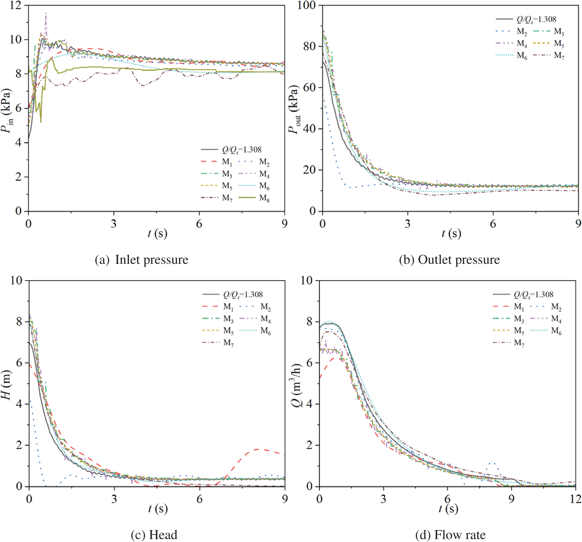
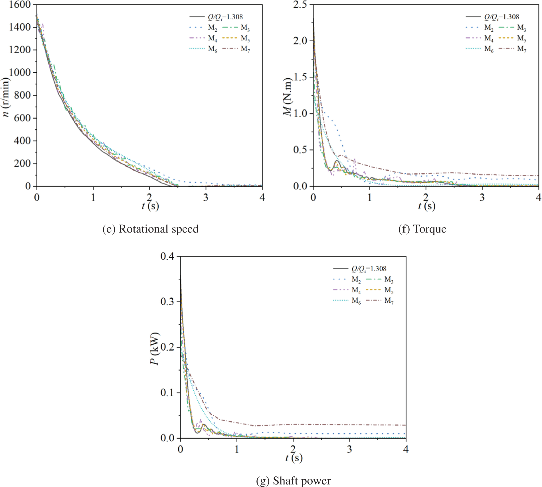
Figure 20: Power frequency stopping mode external characteristics prediction

In Fig. 20b, six models predicting the outlet pressure are presented, all of which exhibit a consistent trend with the experimental curve: a rapid decrease from 0 to 1.5 s, followed by a slower decrease towards a stable value. Specifically, the M2 curve shows a rapid decline from 0 to 2 s, but it is significantly lower than the experimental curve during this period; however, after stabilization, it aligns well with the stable value of the experimental curve, with an average absolute error of 0.0029 kPa and an average relative error of 11.48%. The M3 to M5 curves closely match the experimental data from 0 to 2 s, with slightly higher outlet pressure values, and they stabilize at values consistent with the experimental curve, showing high agreement, with average absolute errors of 0.0016, 0.0015, and 0.0016 kPa, and average relative errors of 6.48%, 6.32%, and 6.81%, respectively. The M6 and M7 curves have slightly higher outlet pressure values than the experimental data from 0 to 2 s and then become slightly lower from 2 to 7 s, stabilizing later; the M6 curve matches the stable value of the experimental curve, while the M7 curve stabilizes at a slightly lower value, with average absolute errors of 0.0019 and 0.0033 kPa, and average relative errors of 11.66% and 21.35%, respectively. The M1 and M8 curves are omitted from the figure due to unsatisfactory prediction results. Based on the average relative and absolute errors, the M3 to M6 models demonstrate better predictive performance, with the M4 model, the ensemble regression model combining GBTR and RFR, showing the best predictive accuracy.

In Fig. 20c, seven models predicting the head are presented, all of which show an initial rapid decrease followed by a gradual stabilization. Specifically, the M1 curve starts with a lower initial value than the experimental curve, at 5.88 m, and exhibits a slower decrease from 0 to 2 s compared to the experimental data. After t > 6 s, the M1 curve shows a sudden and significant rise, resulting in a large discrepancy from the experimental curve, with an average absolute error of 0.68 m and an average relative error of 158.51%. The M2 curve also begins with a lower initial value than the experimental curve, at 4.45 m, and remains below the experimental values during the 0 to 2 s interval. However, after reaching the stable value, it aligns well with the experimental curve, with an average absolute error of 0.37 m and an average relative error of 30.92%. The M3 to M6 curves show high overall agreement with the experimental data, both in terms of the time to reach the stable value and the magnitude of the stable value, with average absolute errors of 0.15, 0.14, 0.15, and 0.10 m, and average relative errors of 14.85%, 12.74%, 16.72%, and 12.08%, respectively. The M7 curve is generally in good agreement with the experimental data but stabilizes at a slightly lower value, only 0.02 m below the experimental curve, with an average absolute error of 0.31 m and an average relative error of 65.71%. The M8 curve is omitted from the figure due to unsatisfactory prediction results. Based on the average relative and absolute errors, the M3 to M6 models demonstrate better predictive performance, with the M6 model (FNN) showing the best predictive accuracy.

In Fig. 20d, seven flow rate prediction models are presented, all of which exhibit a trend consistent with the experimental curve: a rapid decrease at t = 1 s, followed by a gradual slowing of the flow rate decrease, and ultimately reaching zero. Specifically, the M1 curve starts with an initial value of 5.31 m3/h, which is lower than the experimental curve’s 7.68 m3/h. From 0 to 1 s, the M1 curve shows significant differences from the experimental data, and from 1 to 7 s, the flow rate values are slightly lower, with the M1 curve reaching zero earlier than the experimental curve. The average absolute error is 0.49 m3/h, and the average relative error is 240.40%. The M2 curve shows high agreement with the experimental data from 0 to 5 s but begins to fluctuate after t = 5 s, leading to larger discrepancies and reaching zero slightly earlier than the experimental curve, with an average absolute error of 0.17 m3/h and an average relative error of 38.49%. The M3, M4, and M5 curves show good overall agreement with the experimental data, but their initial flow rates are lower than the experimental curve, and they reach zero earlier. The average absolute errors for M3, M4, and M5 are 0.28 m3/h, and the average relative errors are 16.72%, 19.67%, and 16.46%, respectively. The M6 curve is in high agreement with the experimental data, with an average absolute error of 0.12 m3/h and an average relative error of 44.49%. The M7 curve also shows good agreement, with an initial value slightly lower than the experimental curve, and flow rates that are slightly higher than the experimental data after t > 2 s, though the differences are small. The M7 curve does not reach zero, stabilizing at approximately 0.14 m3/h, with an average absolute error of 0.24 m3/h and an average relative error of 137.53%.The M8 curve is omitted from the figure due to unsatisfactory prediction results. Based on the average relative and absolute errors, the M3 to M7 models demonstrate better predictive performance, with the M6 model (FNN) showing the best predictive accuracy.

In Fig. 20e, six models predicting the rotational speed are presented, all of which exhibit a trend consistent with the experimental curve: an initial rapid decrease, followed by a gradual slowing of the decrease, and ultimately reaching zero. Specifically, the M2 curve aligns well with the experimental data from 0 to 1 s, but after t > 1 s, the M2 rotational speed values gradually become higher than those of the experimental curve, and it reaches zero at t = 4 s, which is later than the experimental curve, with an average absolute error of 23.80 r/min. The M3 to M5 curves show high overall agreement with the experimental data; as time progresses, the difference in rotational speed between these curves and the experimental curve increases slightly, but the increase is minimal, with average absolute errors of 9.80, 6.51, and 6.52 r/min, respectively. The M6 curve follows the same trend as the experimental curve, but its rotational speed values are consistently slightly higher, with an average absolute error of 17.22 r/min. The M7 curve shows high agreement with the experimental data, with an average absolute error of 8.94 r/min.The M1 and M8 curves are omitted from the figure due to unsatisfactory prediction results. Based on the average absolute errors, the M3, M4, M5, and M7 models demonstrate better predictive performance, with the M4 model, the ensemble regression model combining GBTR and RFR, showing the best predictive accuracy. Due to the small values of the experimental curve, the relative errors are not considered informative for evaluation and are therefore not used as a criterion.

In Fig. 20f, six models predicting the torque are presented, and all of the prediction curves exhibit a consistent trend with the experimental curve: an initial rapid decrease, followed by a slower decrease, and ultimately reaching zero. Specifically, the M2 curve shows high agreement with the experimental data for t < 0.2 s, but afterwards, the torque values are consistently higher than those of the experimental curve, with significant differences, resulting in an average absolute error of 0.10 N·m. The M3, M4, and M5 curves show high overall agreement with the experimental data; the M4 curve exhibits minor fluctuations during the process, but all three models demonstrate good predictive performance, with an average absolute error of 0.01 N·m for each. The M6 curve shows slight discrepancies from the experimental data between 0 and 0.5 s, but it aligns well with the experimental curve for t > 0.5 s, with an average absolute error of 0.04 N·m. The M7 curve follows the general trend of the experimental data, but its torque values are consistently higher, and it does not reach zero, instead stabilizing at approximately 0.15 N·m, with an average absolute error of 0.13 N·m. The M1 and M8 curves are omitted from the figure due to unsatisfactory prediction results. Based on the average absolute errors, the M3 to M7 models demonstrate better predictive performance, with the M5 model (KNNR) showing the best predictive accuracy. Due to the small values of the experimental curve, relative errors are not considered informative for evaluation and are therefore not used as a criterion.

In Fig. 20g, six models predicting the shaft power are presented, and all of the prediction curves exhibit a consistent trend with the experimental curve: an initial rapid decrease, followed by a slower decline, and ultimately reaching zero. Specifically, the M2 curve shows high agreement with the experimental data from 0 to 0.15 s, but for t > 1.5 s, it gradually diverges from the experimental curve, with shaft power values higher than the experimental values. The M2 curve does not reach zero, instead stabilizing at approximately 0.0147 kW, with an average absolute error of 0.0128 kW. The M3, M4, and M5 curves show high overall agreement with the experimental data, and they all reach zero at t = 1.91 s, with average absolute errors of 0.0012, 0.0014, and 0.0004 kW, respectively. The M6 curve starts with a lower initial value than the experimental curve and decreases at a slower rate. It shows slight discrepancies from the experimental data between 0 and 0.8 s and reaches zero at t = 1.4 s, earlier than the experimental curve, with an average absolute error of 0.0043 kW. The M7 curve also begins with a lower initial value than the experimental curve, but its shaft power values are consistently higher throughout. The M7 curve does not reach zero, instead stabilizing at approximately 0.03 kW, with an average absolute error of 0.0285 kW. The M1 and M8 curves are omitted from the figure due to unsatisfactory prediction results. Based on the average absolute errors, the M3 to M5 models demonstrate better predictive performance, with the M5 model (KNNR) showing the best predictive accuracy. Due to the small values of the experimental curve, relative errors are not considered informative for evaluation and are therefore not used as a criterion.

Table 3 presents the mean absolute errors and mean relative errors of the external characteristic curves predicted by each machine learning model compared to the experimental curves during power frequency stopping. Prediction methods that exhibited excessively large average errors for certain external characteristic parameters have been excluded from the table for reference purposes. From the table, it can be observed that Models M2 to M7 achieved relatively high prediction accuracy across all parameters, rendering their results more reliable. In contrast, Models M1 and M8 generally performed poorly in terms of prediction accuracy. For the prediction of inlet and outlet pressures, all methods achieved satisfactory results. However, it is noteworthy that for the prediction of rotational speed, torque, and shaft power, the mean absolute errors were small, but the mean relative errors were extremely large. This is due to the fact that the experimental values of these parameters rapidly decreased to values very close to zero, leading to very small denominators in the relative error calculations and thus resulting in extremely large relative errors. Consequently, these relative errors are not considered as reliable references. Models M1 and M7 exhibited excessively large mean relative errors when predicting head and flow rate. This is because, after the experimental values decreased to near-zero, the predicted values remained at relatively high levels, leading to significant discrepancies.

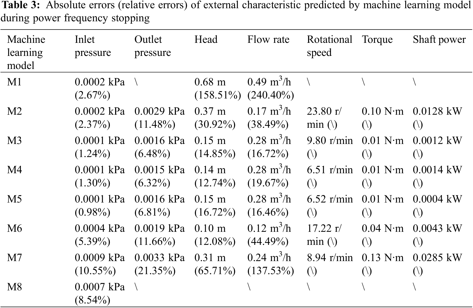
4.4 Frequency Conversion Starting Mode Performance Prediction

In Fig. 21, the prediction of seven external characteristic curves for the experimental pump at a steady-state flow rate ratio of Q/Qr = 1.296 during starting in frequency conversion mode is shown. Fig. 21a presents the experimental curve and five different model predictions for the inlet pressure, all of which exhibit an initial decrease followed by small fluctuations around a stable value. The M1 curve aligns well with the experimental data from 0 to 1.5 s and continues to show small fluctuations close to the experimental curve after t > 1.5 s, demonstrating overall good agreement. The average absolute error is 0.0003 kPa, and the average relative error is 6.97%. The M2, M3, and M5 curves match the experimental data from 0 to 2 s but gradually diverge after t > 2 s, with their inlet pressure values consistently higher than those of the experimental curve. The average absolute errors are 0.0010, 0.0009, and 0.0009 kPa, and the average relative errors are 20.72%, 19.42%, and 19.12%, respectively. The M7 curve shows good agreement with the experimental data from 0.5 to 3 s; however, during the 0 to 0.5 s interval, the inlet pressure values are significantly lower than the experimental curve, and after t > 3 s, the inlet pressure values are significantly higher than the experimental curve. The average absolute error is 0.0010 kPa, and the average relative error is 20.16%. The M4, M6, and M8 curves are omitted from the figure due to unsatisfactory prediction results. Based on the average relative and absolute errors, only the M1 model (SVMR) demonstrates satisfactory predictive performance.

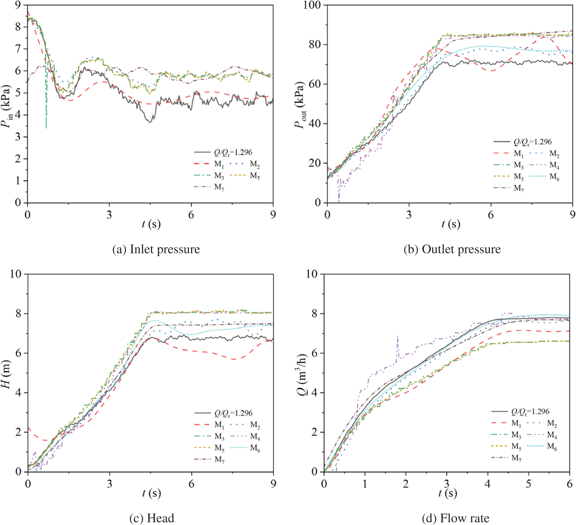
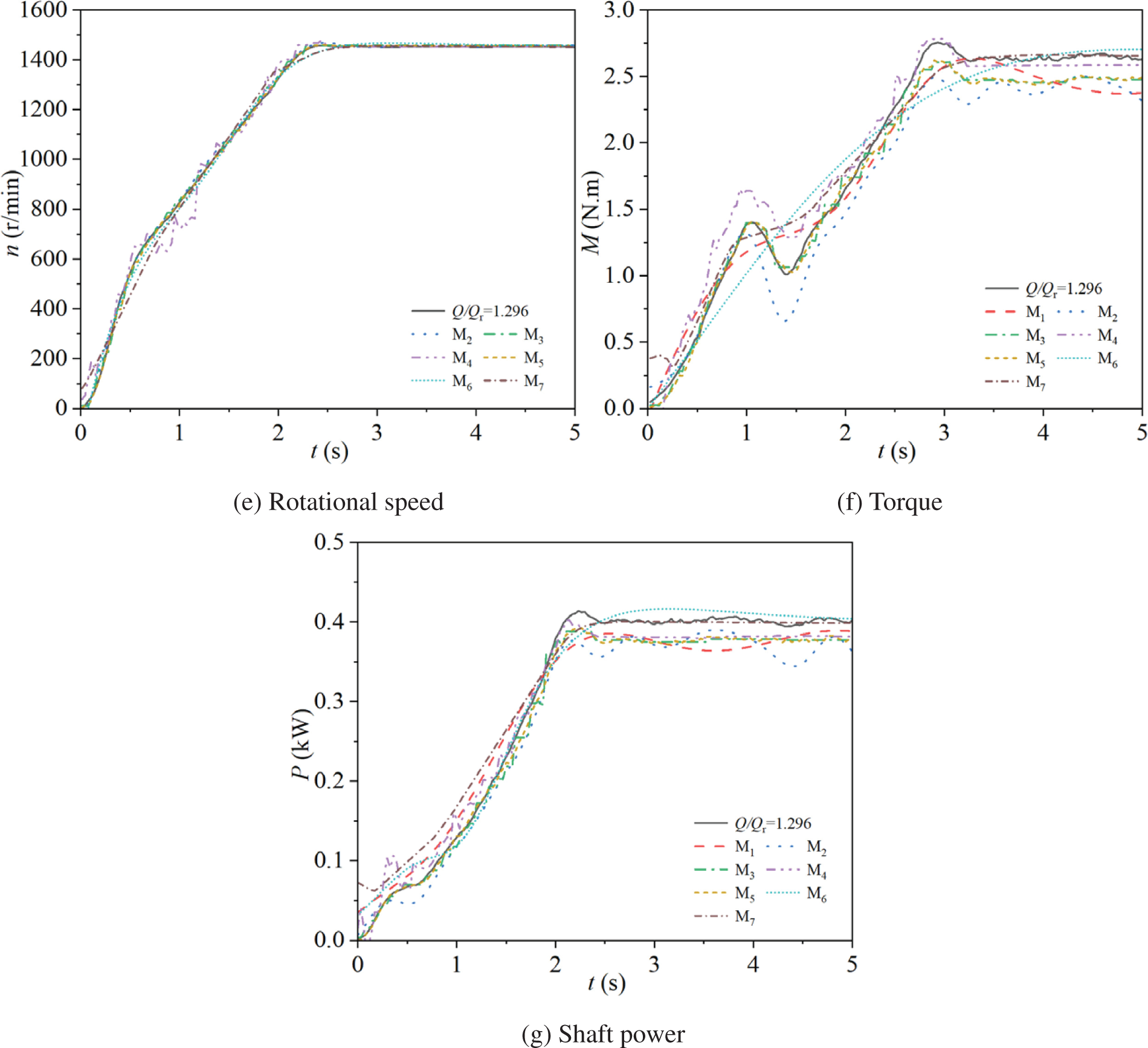
Figure 21: Frequency conversion starting mode external characteristics prediction

In Fig. 21b, the experimental curve and seven different model predictions for the outlet pressure are presented, all of which exhibit a rapid increase followed by stabilization at a steady value. The M1 curve shows high agreement with the experimental data from 0 to 1 s but gradually diverges after t > 1 s, with outlet pressure values becoming higher than those of the experimental curve. It eventually fluctuates within a relatively large range around the stable value of the experimental curve, with an average absolute error of 0.0059 kPa and an average relative error of 10.70%. The M2 curve aligns well with the experimental data during the rapid increase phase from 0 to 4 s, but it stabilizes at a value higher than the experimental curve, with an average absolute error of 0.0038 kPa and an average relative error of 6.08%. The M3, M5, M6, and M7 curves show good agreement with the experimental data from 0 to 1 s, but after t > 1 s, their outlet pressure values become higher than the experimental curve, and they stabilize at values higher than the experimental steady state. Among these, the M6 curve stabilizes at a value closer to the experimental curve. The average absolute errors are 0.0103, 0.0102, 0.0049, and 0.0096 kPa, and the average relative errors are 16.40%, 16.10%, 8.55%, and 14.92%, respectively. The M4 curve fluctuates within a range close to the experimental outlet pressure values throughout, and it also stabilizes at a value higher than the experimental steady state, with an average absolute error of 0.0108 kPa and an average relative error of 20.13%. The M8 curve is omitted from the figure due to unsatisfactory prediction results. Based on the average relative and absolute errors, the M2 and M6 models demonstrate better predictive performance, with the M2 model (GPR) showing the best predictive accuracy.

In Fig. 21c, the experimental curve and seven different model predictions for the head are presented, all of which exhibit an initial rapid increase followed by stabilization at a steady value. The M1 curve aligns well with the experimental data from 1 to 4 s. However, during the 0 to 1 s interval, the head values are higher than those of the experimental curve, and the initial value does not start from zero. After t > 4 s, while the experimental curve fluctuates slightly around the stable value, the M1 curve does not stabilize and remains slightly below the experimental curve’s head value, with an average absolute error of 0.55 m and an average relative error of 27.75%. The M2 curve shows high agreement with the experimental data during the rapid increase phase from 0 to 4 s. However, after the experimental curve reaches a stable head, the M2 curve fluctuates around 7.43 m, which is higher than the stable value of the experimental curve, with an average absolute error of 0.40 m and an average relative error of 9.25%. The M3, M4, and M5 curves show good agreement with the experimental data from 0 to 1 s. However, after t > 1 s, their head values gradually become higher than the experimental curve, and they stabilize at values higher than the experimental steady state. The average absolute errors are 0.93, 0.93, and 0.92 m, and the average relative errors are 16.24%, 20.90%, and 16.00%, respectively. The M6 and M7 curves align well with the experimental data from 0 to 4 s but ultimately stabilize at values higher than the experimental steady state. The average absolute errors are 0.40 and 0.49 m, and the average relative errors are 14.88% and 11.47%, respectively. The M8 curve is omitted from the figure due to unsatisfactory prediction results. Based on the average relative and absolute errors, the M2, M6, and M7 models demonstrate better predictive performance, with the M2 model (GPR) showing the best predictive accuracy.

In Fig. 21d, the experimental curve and seven different model predictions for the flow rate are presented, all of which exhibit an initial rapid increase, followed by a gradual increase, and finally stabilization at a certain value. The M1, M3, and M5 curves align well with the experimental data during the rapid increase phase from 0 to 1 s. However, in the 1 to 4 s interval, where the flow rate gradually increases, these three prediction curves show lower flow rates than the experimental curve, and they stabilize at values lower than the experimental steady state. The average absolute errors are 0.70, 0.93, and 0.93 m3/h, and the average relative errors are 16.84%, 14.92%, and 14.60%, respectively. The M2 curve shows high overall agreement with the experimental data, with flow rate values slightly lower than the experimental curve throughout the entire time span. The average absolute error is 0.30 m3/h, and the average relative error is 17.19%. The M4 curve fluctuates within a range close to the experimental flow rate values but significantly exceeds the experimental flow rate values from 1 to 3.5 s. The average absolute error is 0.37 m3/h, and the average relative error is 41.32%. The M6 curve shows high agreement with the experimental data, with an average absolute error of 0.10 m3/h and an average relative error of 3.72%. The M7 curve also aligns well with the experimental data, showing only small fluctuations around the experimental flow rate values. The average absolute error is 0.24 m3/h, and the average relative error is 12.89%. The M8 curve is omitted from the figure due to unsatisfactory prediction results. Based on the average relative and absolute errors, the M2, M6, and M7 models demonstrate better predictive performance, with the M6 model (FNN) showing the best predictive accuracy.

In Fig. 21e, the experimental curve and six different model predictions for the rotational speed are presented, all of which exhibit an initial rapid increase, followed by a slightly slower but still rapid increase, and finally stabilization at a certain value. The M2, M3, M5, and M6 curves show high overall agreement with the experimental data, reaching the stable value at the same time and magnitude as the experimental curve, with the exception that the M6 curve stabilizes slightly later than the experimental curve. The average absolute errors are 5.05, 5.69, 3.70, and 9.42 r/min, respectively, and the average relative errors are 7.46%, 2.89%, 0.63%, and 24.47%, respectively. The M4 and M7 curves align well with the experimental data from 0 to 2.5 s, showing only occasional small fluctuations around the experimental rotational speed values. After reaching the stable value, both curves remain consistent with the experimental curve, with the M7 curve stabilizing slightly later. The average absolute errors are 9.09 and 13.00 r/min, and the average relative errors are 11.39% and 21.54%, respectively. The M1 and M8 curves are omitted from the figure due to unsatisfactory prediction results. Based on the average relative and absolute errors, the M2 to M6 models demonstrate better predictive performance, with the M5 model (KNNR) showing the best predictive accuracy.

In Fig. 21f, the experimental curve and seven different model predictions for the torque are presented, all of which exhibit an initial increase followed by stabilization. The M2 to M5 curves show a similar behavior to the experimental curve during the 1 to 1.5 s interval, where there is a fluctuation and a decrease in torque values. In contrast, the M1 and M7 curves only show a slight deceleration in the rate of torque change during this period, while the M6 curve does not exhibit any particular changes. The M1, M6, and M7 curves differ significantly from the experimental trend. The M7 curve aligns with the experimental curve after reaching the stable value. The average absolute errors are 0.22, 0.07, and 0.05 N·m, and the average relative errors are 11.28%, 4.69%, and 8.86%, respectively. The M2 curve shows a lower trough at t = 1.5 s compared to the experimental curve and stabilizes at a value lower than the experimental steady state, with an average absolute error of 0.24 N·m and an average relative error of 12.04%. The M3 and M5 curves align well with the experimental data from 0 to 2.5 s but ultimately stabilize at values lower than the experimental steady state, with average absolute errors of 0.14 and 0.14 N·m, and average relative errors of 6.90% and 7.05%, respectively. The M4 curve is slightly higher than the experimental torque values from 0 to 2 s but stabilizes at a value close to the experimental steady state, with an average absolute error of 0.09 N·m and an average relative error of 9.24%. The M8 curve is omitted from the figure due to unsatisfactory prediction results. Based on the average relative and absolute errors, the M3 to M7 models demonstrate better predictive performance, with the M7 model (DLN) showing the best predictive accuracy.

In Fig. 21g, the experimental curve and seven different model predictions for the shaft power are presented, all of which exhibit an initial rapid increase followed by stabilization at a certain value. The M1, M2, and M4 curves align well with the experimental data from 0 to 2 s. The M1 curve shows slightly higher shaft power values than the experimental curve, while the M2 and M4 curves fluctuate within a small range around the experimental shaft power values. The M3 and M5 curves also show high agreement with the experimental data from 0 to 2 s, with good fitting. However, all five curves (M1, M2, M3, M4, M5) stabilize at values slightly lower than the experimental steady state. The average absolute errors are 0.0347, 0.0325, 0.0216, 0.0226, and 0.0232 kW, and the average relative errors are 26.00%, 12.51%, 7.33%, 15.99%, and 5.93%, respectively. The M6 curve is slightly higher than the experimental shaft power values from 0 to 1 s and then aligns well with the experimental data from 1 to 2 s. However, after reaching its peak, it does not stabilize but instead decreases slowly, gradually approaching the experimental steady state. The average absolute error is 0.0119 kW, and the average relative error is 19.26%. The M7 curve is also slightly higher than the experimental shaft power values from 0 to 2 s. After stabilization, it matches the experimental steady state, showing high agreement with the experimental curve. The average absolute error is 0.0127 kW, and the average relative error is 40.30%. The M8 curve is omitted from the figure due to unsatisfactory prediction results. Based on the average relative and absolute errors, the M1 to M6 models demonstrate better predictive performance, with the M6 model (FNN) showing the best predictive accuracy.

Table 4 presents the mean absolute errors and mean relative errors of the external characteristic curves predicted by each machine learning model compared to the experimental curves during frequency conversion starting. Prediction methods that exhibited excessively large average errors for certain external characteristic parameters have been excluded from the table for reference purposes. From the table, it can be observed that, with the exception of Model M8, all other prediction methods achieved low mean absolute and relative errors, indicating generally good prediction performance. The results obtained using these methods are more reliable. Compared to power frequency starting, the errors in predicting the external characteristics during frequency conversion starting are smaller, and the prediction performance is better. This is because, during frequency conversion starting, the fluctuations in the parameters before reaching steady-state values are smaller, and the time taken to reach steady state is longer, leading to less uncertainty and easier prediction. Notably, Models M1 and M7, which performed poorly in predicting the external characteristics during power frequency starting, also achieved better results during frequency conversion starting.

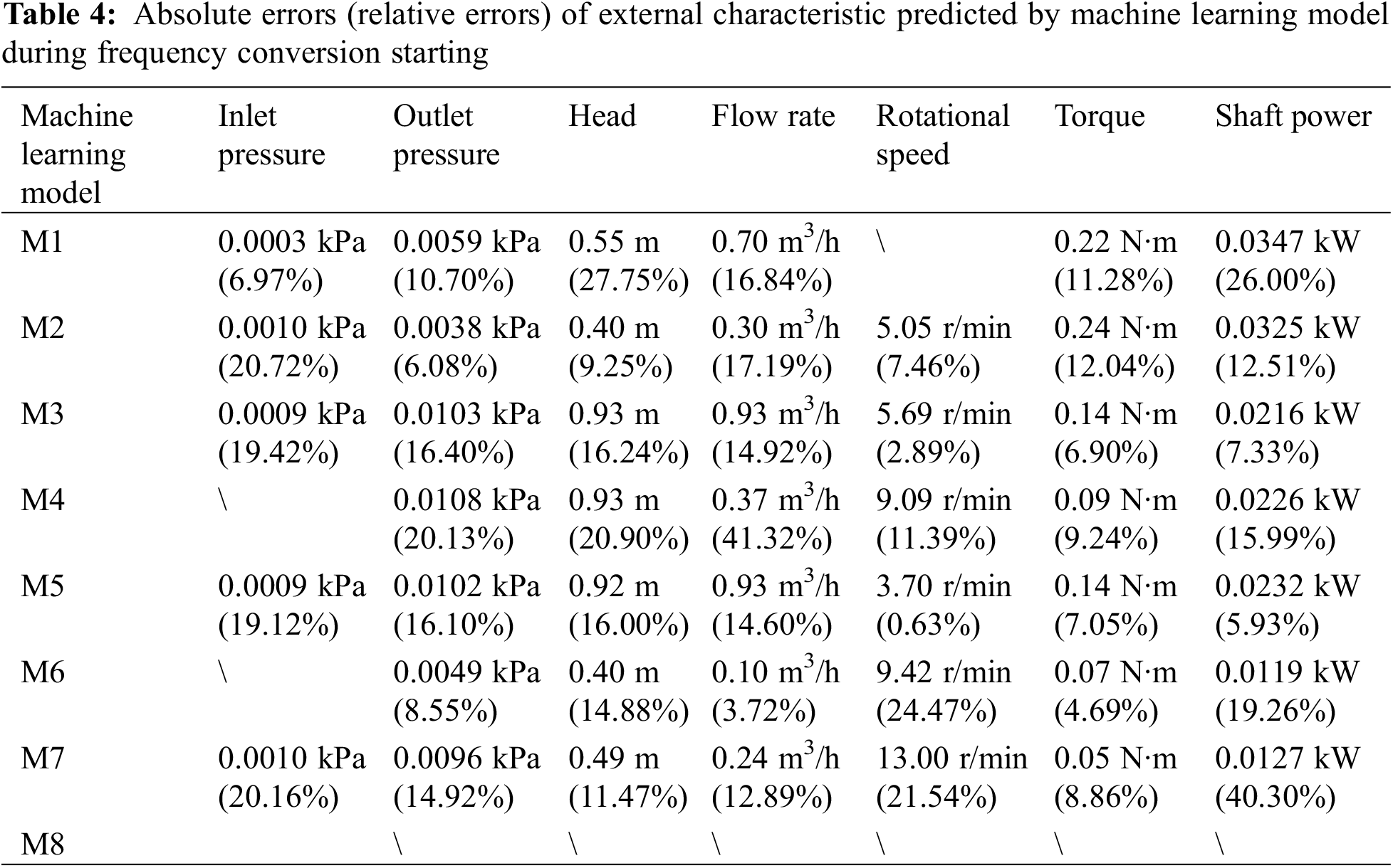
4.5 Frequency Conversion Stopping Mode Performance Prediction

In Fig. 22, the prediction of seven external characteristic curves for the experimental pump at a steady-state flow rate ratio of Q/Qr = 1.296 during stopping in frequency conversion mode is shown. Fig. 22a presents the comparison between the experimental curve and five different model predictions for the inlet pressure, which generally exhibit an initial rapid increase followed by a slow decrease to a stable value. The M1 curve aligns well with the experimental data from 0 to 3 s and shows high agreement after t > 3 s. The overall trend of the M1 curve is smoother compared to the experimental curve, with an average absolute error of 0.0002 kPa and an average relative error of 2.13%. The M2 curve starts with a higher initial value than the experimental curve. From 0 to 2 s, the inlet pressure values are higher than those of the experimental curve. After t > 2 s, the M2 curve aligns well with the experimental curve, with slightly lower inlet pressure values, and it stabilizes at a value that is also slightly lower than the experimental curve. The average absolute error is 0.0002 kPa, and the average relative error is 3.18%. The M3, M4, and M5 curves show significant differences from the experimental data from 0 to 3 s, with inlet pressure values higher than the experimental curve. Notably, the M4 curve exhibits a large fluctuation in inlet pressure values between 0.5 and 1.5 s, significantly exceeding the experimental values. However, after t > 3 s, all three curves show high agreement with the experimental curve, stabilizing at consistent values. The average absolute errors for M3, M4, and M5 are all 0.0002 kPa, and the average relative errors are 2.41%, 3.29%, and 2.36%, respectively. The M6, M7, and M8 curves are omitted from the figure due to unsatisfactory prediction results. Based on the average relative and absolute errors, the M1 to M5 models demonstrate good predictive performance, with the M1 model (SVMR) showing the best predictive accuracy.

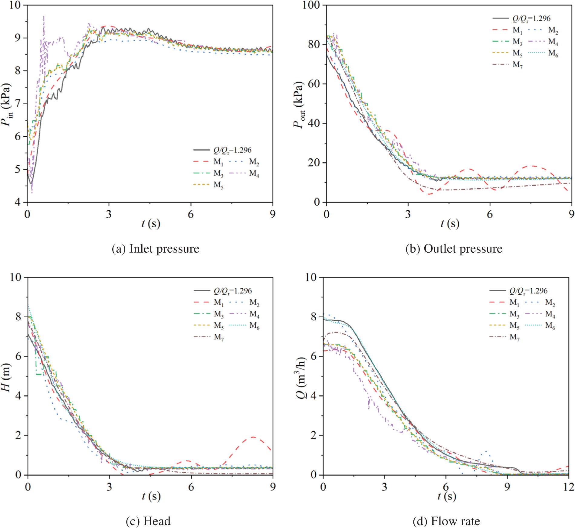
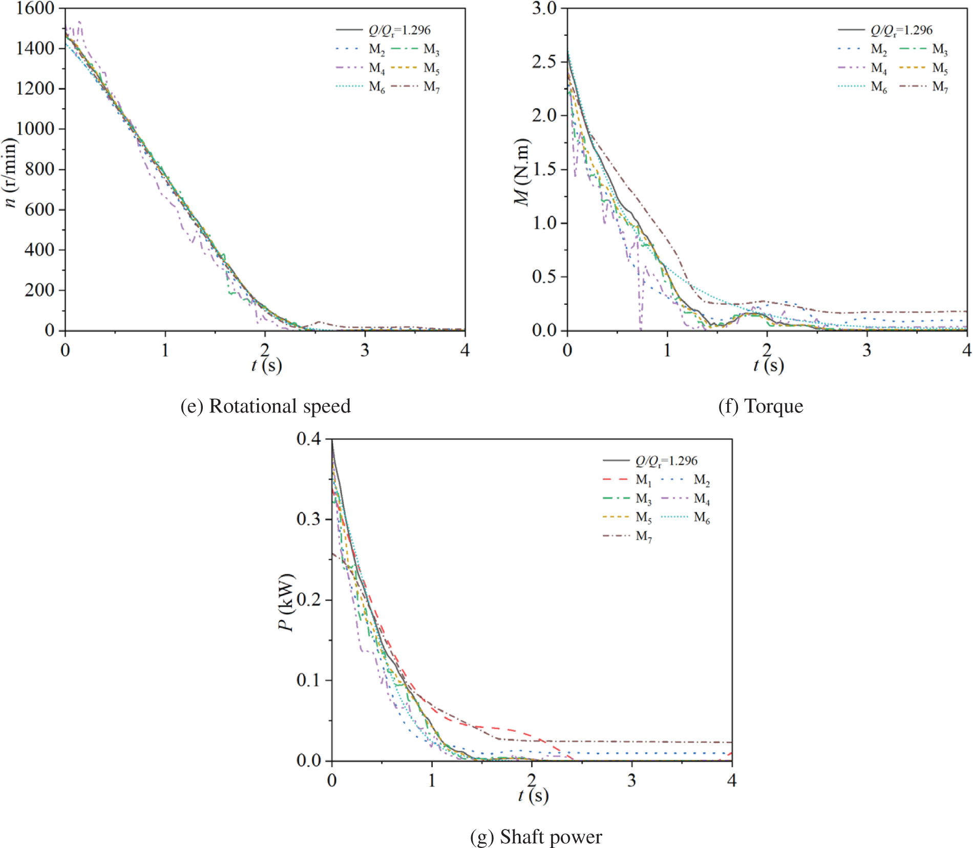
Figure 22: Frequency conversion stopping mode external characteristics prediction

In Fig. 22b, the experimental curve and seven different model predictions for the outlet pressure during stopping in frequency conversion mode are presented. The outlet pressure generally exhibits a rapid decrease followed by stabilization around a steady value. The M1 curve aligns well with the experimental data from 0 to 1.5 s, with predicted values close to the experimental values. However, after t > 1.5 s, it begins to fluctuate around the experimental values and ultimately oscillates within a relatively large range near the stable value of the experimental curve. The average absolute error is 0.0039 kPa, and the average relative error is 27.05%. The M2 curve shows high overall agreement with the experimental data, with predicted values very close to the experimental values. The average absolute error is 0.0007 kPa, and the average relative error is 4.36%. The M3, M4, M5, and M6 curves exhibit consistent trends with the experimental curve from 0 to 3 s, but their predicted values are slightly higher than the experimental values. After t > 3 s, all four curves show high agreement with the experimental curve, with predicted values very close to the experimental values, and they stabilize at almost the same time and magnitude as the experimental curve. The average absolute errors are 0.0021, 0.0022, 0.0021, and 0.0015 kPa, and the average relative errors are 6.65%, 7.58%, 6.11%, and 5.45%, respectively. The M7 curve has predicted values slightly higher than the experimental values from 0 to 1.5 s. After t > 1.5 s, the predicted values become slightly lower than the experimental values. The outlet pressure decreases to a minimum and then slowly increases, gradually approaching the stable value of the experimental curve. The average absolute error is 0.0038 kPa, and the average relative error is 25.16%. The M8 curve is omitted from the figure due to unsatisfactory prediction results. Based on the average relative and absolute errors, the M2 to M6 models demonstrate better predictive performance, with the M2 model (GPR) showing the best predictive accuracy.

In Fig. 22c, the experimental curve and seven different model predictions for the head during stopping in frequency conversion mode are presented. All curves exhibit a rapid decrease in head, followed by stabilization at a steady value. The M1 curve aligns well with the experimental data for t < 3 s, with predicted values close to the experimental values. However, after t > 3 s, it begins to diverge significantly from the experimental curve, showing large fluctuations around the stable value of the experimental curve. The average absolute error is 0.63 m, and the average relative error is 164.85%. The M2 to M5 curves show good agreement with the experimental data from 0 to 2 s. After t > 2 s, these curves maintain high alignment with the experimental curve, with predicted values very close to the experimental values. They also stabilize at almost the same time and magnitude as the experimental curve. The average absolute errors are 0.19, 0.15, 0.11, and 0.15 m, and the average relative errors are 25.61%, 12.05%, 15.19%, and 12.61%, respectively. The M6 curve has slightly higher head values than the experimental data for t < 1 s. After that, it shows high agreement with the experimental curve, with predicted values very close to the experimental values. The average absolute error is 0.11 m, and the average relative error is 13.17%. The M7 curve aligns well with the experimental data for t < 5 s, with predicted values very close to the experimental values. However, after t > 5 s, the predicted head values drop slightly, stabilizing at a value that is slightly lower than the experimental curve’s stable value. The average absolute error is 0.27 m, and the average relative error is 58.64%. The M8 curve is omitted from the figure due to unsatisfactory prediction results. Based on the average relative and absolute errors, the M2 to M6 models demonstrate better predictive performance, with the M6 model (FNN) showing the best predictive accuracy.

In Fig. 22d, the experimental curve and seven different model predictions for the flow rate during stopping in frequency conversion mode are presented. All curves generally exhibit a smooth transition, followed by a rapid decrease, and then a gradual decline to zero. The M1 curve is slightly lower than the experimental flow rate values for t < 4 s. From 4 to 7 s, it aligns well with the experimental curve. After t > 7 s, it fluctuates around the experimental values. The average absolute error is 0.55 m3/h, and the average relative error is 225.25%. The M2 curve shows good agreement with the experimental data for t < 5 s, with predicted values slightly lower than the experimental values. Between 5 and 9 s, it exhibits fluctuations around the experimental values and reaches zero at t = 9 s, which is slightly earlier than the experimental curve. The average absolute error is 0.25 m3/h, and the average relative error is 35.88%. The M3, M4, and M5 curves follow a trend similar to the experimental curve but have overall predicted values that are slightly lower. They also reach zero slightly earlier than the experimental curve. The average absolute errors are 0.42, 0.60, and 0.41 m3/h, and the average relative errors are 23.29%, 25.26%, and 23.19%, respectively. The M6 curve shows high agreement with the experimental data for t < 7 s, with predicted values very close to the experimental values. From 7 to 10 s, the predicted values are slightly lower than the experimental values, and it reaches zero at the same time as the experimental curve. The average absolute error is 0.10 m3/h, and the average relative error is 28.15%. The M7 curve aligns well with the experimental curve overall, with predicted values slightly lower than the experimental values from 0 to 2 s. After t > 2 s, the difference between the predicted and experimental values is not significant. The average absolute error is 0.23 m3/h, and the average relative error is 117.05%. The M8 curve is omitted from the figure due to unsatisfactory prediction results. Based on the average relative and absolute errors, the M2, M3, M5, and M6 models demonstrate better predictive performance, with the M6 model (FNN) showing the best predictive accuracy.

In Fig. 22e, the experimental curve and six different model predictions for the rotational speed during stopping in frequency conversion mode are presented. All curves show a rapid decrease followed by a gradual decline to zero. The M2, M3, M5, and M6 curves show high overall agreement with the experimental data, with predicted values very close to the experimental values. These models all reach zero at the same time as the experimental curve. The average absolute errors are 8.96, 3.58, 1.46, and 9.76 r/min, respectively. The M4 curve aligns well with the experimental data but shows small fluctuations around the experimental values, making it slightly more oscillatory than the experimental curve. The average absolute error is 12.02 r/min. The M7 curve shows high agreement with the experimental data from 0 to 2.5 s, with predicted values very close to the experimental values. However, after the experimental value drops to zero, the M7 curve does not reach zero but stabilizes at approximately 17 r/min. The average absolute error is 10.72 r/min. The M1 and M8 curve is omitted from the figure due to unsatisfactory prediction results. Based on the average absolute errors, the M3 and M5 models demonstrate better predictive performance, with the M5 model (KNNR) showing the best predictive accuracy. Since the experimental values are very small, relative errors do not provide a meaningful comparison and are therefore not used as an evaluation criterion.

In Fig. 22f, the experimental curve and six different model predictions for the torque during stopping in frequency conversion mode are presented. All curves generally show a rapid decrease followed by a gradual decline to zero. The M2 curve is slightly lower than the experimental torque values from 0 to 1 s. After t > 1 s, the predicted values become slightly higher than the experimental values, and it stabilizes at 0.1 N·m without reaching zero. The average absolute error is 0.11 N·m. The M3 and M5 curves align well with the experimental data for t < 0.7 s, with predicted values slightly lower than the experimental values. After t > 0.7 s, both curves show high agreement with the experimental curve, with predicted values very close to the experimental values, and they reach zero at the same time as the experimental curve. The average absolute errors are 0.02 and 0.01 N·m, respectively. The M4 curve has predicted values lower than the experimental values from 0 to 1.5 s and shows significant fluctuations. After t > 1.5 s, it aligns well with the experimental curve, with a small difference between the predicted and experimental values. The average absolute error is 0.05 N·m. The M6 curve is smoother than the experimental curve and shows high agreement for t < 1 s. Between 1 and 2 s, the predicted torque values are higher than the experimental values. After t > 2 s, it aligns well with the experimental curve, with predicted values slightly higher than the experimental values. The average absolute error is 0.03 N·m. The M7 curve follows a similar trend to the experimental curve but has overall predicted values that are higher than the experimental values. It does not reach zero but stabilizes at approximately 0.18 N·m. The average absolute error is 0.14 N·m. The M1 and M8 curves are omitted from the figure due to unsatisfactory prediction results. Based on the average absolute errors, the M3, M5, and M6 models demonstrate better predictive performance, with the M5 model (KNNR) showing the best predictive accuracy. Since the experimental values are very small, relative errors do not provide meaningful information and are therefore not used as an evaluation criterion.

In Fig. 22g, the experimental curve and seven different model predictions for the shaft power during stopping in frequency conversion mode are presented. All curves generally exhibit a rapid decrease followed by stabilization. The M1 curve aligns well with the experimental data for t < 0.75 s but shows significant differences after t > 0.75 s, with large fluctuations around zero. The average absolute error is 0.0212 kW. The M2 curve has predicted values slightly lower than the experimental values from 0 to 1 s. After t > 1 s, the predicted values become slightly higher than the experimental values and stabilize at approximately 0.01 kW without reaching zero. The average absolute error is 0.0143 kW. The M3 and M4 curves show good overall agreement with the experimental data. From 0 to 1 s, the predicted values are slightly lower than the experimental values, and after t > 1 s, they align well with the experimental curve, stabilizing at zero at the same time as the experimental curve. The average absolute errors are 0.0020 and 0.0046 kW, respectively. The M5 and M6 curves also show high agreement with the experimental data, aligning well throughout and reaching zero at the same time as the experimental curve. The average absolute errors are 0.0012 and 0.0029 kW, respectively. The M7 curve aligns well with the experimental data from 0.3 to 0.8 s. However, for t < 0.3 s, the predicted values are lower than the experimental values, and after t > 0.8 s, the predicted values are higher than the experimental values, stabilizing at approximately 0.03 kW without reaching zero. The average absolute error is 0.0218 kW. The M8 curve is omitted from the figure due to unsatisfactory prediction results. Based on the average absolute errors, the M3, M4, M5, and M6 models demonstrate better predictive performance, with the M5 model (KNNR) showing the best predictive accuracy. Since the experimental values are very small, relative errors do not provide meaningful information and are therefore not used as an evaluation criterion.

Table 5 presents the mean absolute errors and mean relative errors of the external characteristic curves predicted by each machine learning model compared to the experimental curves during frequency conversion stopping. Prediction methods that exhibited excessively large average errors for certain external characteristic parameters have been excluded from the table for reference purposes. From the table, it can be observed that, with the exception of Model M8, all other prediction methods achieved low mean absolute errors, indicating generally good prediction performance. The results obtained using these methods are more reliable. When predicting rotational speed, torque, and head, the experimental values rapidly decrease to near-zero values, leading to very small denominators in the relative error calculations and, consequently, extremely large relative errors. Therefore, these relative errors are not used as a reference. Similarly, the large relative errors in the predictions of head and flow rate by Models M1 and M7 are also due to the same reason. Unlike during starting, the prediction performance during power frequency stopping is comparable to that during frequency conversion stopping, maintaining a similar level of accuracy. This is because, during stopping, the two modes do not exhibit significant differences, and the fluctuations and time taken to reach steady-state values are relatively similar.

5  Conclusion

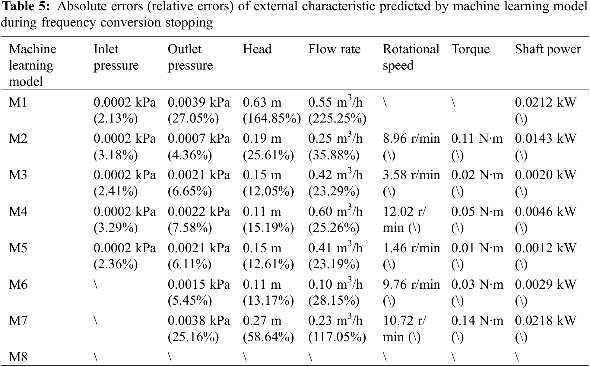
This paper conducted an experimental investigation on the external characteristics of a five-bladed closed impeller centrifugal pump during starting and stopping processes in both power frequency and frequency conversion operation modes. The external characteristics were predicted using eight different machine learning models. Through a comparative experimental analysis of power frequency and frequency conversion starting methods, this study has elucidated the time-dependent variation curves of the primary hydraulic parameters of a centrifugal pump under different starting conditions, providing data support for research on pump starting and stopping processes. Additionally, by employing eight distinct machine learning models to predict these key parameters, the study has identified the most suitable predictive approaches for each parameter. This work lays a theoretical foundation for future predictions of centrifugal pump hydraulic performance. The specific conclusions are as follows:

(1) During the starting process, the external characteristics of the pump in frequency conversion operation reached a steady state later than those in power frequency operation, and the fluctuations before reaching the steady state was less pronounced in the frequency conversion mode. These two features were not significantly observed during the stopping process.

(2) For both starting modes, the outlet pressure, head, flow rate, and rotational speed of the pump increased rapidly over time and then stabilized. In both power frequency and frequency conversion modes, the inlet pressure exhibited significant fluctuations before stabilizing. In the power frequency mode, the torque and shaft power increased rapidly initially, then decreased quickly, and finally stabilized. In the frequency conversion mode, the torque and shaft power increased rapidly and then stabilized, with the torque showing fluctuations during its rapid increase. During the stopping process, the outlet pressure, head, flow rate, rotational speed, torque, and shaft power for both stopping modes decreased rapidly to zero or stabilized at a low value. The outlet pressure for both stopping modes increased rapidly at first and then gradually stabilized.

(3) As the steady-state flow rate increased, the stable values of the inlet pressure, outlet pressure, and head decreased for both power frequency and frequency conversion pumps during starting, while the stable values of the torque and shaft power increased, with no significant change in rotational speed. During stopping, as the steady-state flow rate increased, the time required for the inlet pressure to reach a stable value increased, the time for the outlet pressure and head to decrease to a stable value decreased, and the time for the flow rate to drop to zero increased. The torque and shaft power did not show significant changes. The time for the rotational speed to drop to zero decreased in the power frequency mode, whereas there was no significant change in the frequency conversion mode.

(4) Gaussian Process Regression (GPR), Decision Tree Regression (DTR), an ensemble regression model combining Gradient Boosting Trees Regression (GBTR) and Random Forest Regression (RFR), K-Nearest Neighbors Regression (KNNR), Feedforward Neural Networks (FNN), and Deep Learning Networks (DLN) all demonstrated relatively accurate predictions of the hydraulic performance of the centrifugal pump during starting and stopping. In contrast, Support Vector Machine Regression (SVMR) and Generalized Additive Models (GAM) showed larger prediction errors. Specifically, Gaussian Process Regression (GPR) was more suitable for predicting inlet and outlet pressures, Feedforward Neural Networks (FNN) were more appropriate for predicting head and flow rate, and K-Nearest Neighbors Regression (KNNR) was better suited for predicting rotational speed, torque, and shaft power.

Acknowledgement: None.

Funding Statement: The research was financially supported by Science and Technology Project of Quzhou (Grant Nos. 2023K256, 2023NC08), Research Grants Program of Department of Education of Zhejiang Province (No. Y202455709), Zhejiang Provincial Natural Science Foundation of China (Grant No. LZY21E050001), and University-Enterprise Cooperation Program for Visiting Engineers in Higher Education Institutions in Zhejiang Province (No. FG2020215).

Author Contributions: Yuliang Zhang carried out the transient experiments. Zezhou Yang carried out the performance prediction based on machine learning. Lianghuai Tong proposed the innovative idea. Yanjuan Zhao analyzed the results. Xiaoqi Jia wrote the manuscript. Anda Han revised the manuscript. All authors reviewed the results and approved the final version of the manuscript.

Availability of Data and Materials: The data that support the findings of this study are available from the corresponding author upon reasonable request.

Ethics Approval: None.

Conflicts of Interest: The authors declare no conflicts of interest to report regarding the present study.

References

1. Shojaeefard M, Saremian S. Effects of impeller geometry modification on performance of pump as turbine in the urban water distribution network. Energy. 2022;255(3):124550. doi:10.1016/j.energy.2022.124550. [Google Scholar] [CrossRef]

2. Adiaconitei A, Vintila I, Mihalache R, Alexandru P, Tiberius F, Mihai V, et al. A study on using the additive manufacturing process for the development of a closed pump impeller for mechanically pumped fluid loop systems. Materials. 2021;14(4):967. doi:10.3390/ma14040967. [Google Scholar] [PubMed] [CrossRef]

3. Adiaconitei A, Vintila I, Mihalache R, Alexandru P, Tiberius F, Ionut F, et al. Manufacturing of closed impeller for mechanically pump fluid loop systems using selective laser melting additive manufacturing technology. Materials. 2021;14(20):5908. doi:10.3390/ma14205908. [Google Scholar] [PubMed] [CrossRef]

4. Kumar A, Shandiz M, Sikan F, Mathieu B. Microstructural and mechanical properties of an internal support-free IN625 closed impeller manufactured via laser powder bed fusion (L-PBF). Mater Sci Eng: A. 2023;874(3):145080. doi:10.1016/j.msea.2023.145080. [Google Scholar] [CrossRef]

5. Rezghi A, Riasi A, Tazraei P. Multi-objective optimization of hydraulic transient condition in a pump-turbine hydropower considering the wicket-gates closing law and the surge tank position. Renew Energy. 2020;148:478–91. doi:10.1016/j.renene.2019.10.054. [Google Scholar] [CrossRef]

6. Choi J, Lee G, Kim M. Numerical study on the steady state and transient performance of a multi-type heat pump system. Int J Refrig. 2011;34(2):429–43. doi:10.1016/j.ijrefrig.2010.09.021. [Google Scholar] [CrossRef]

7. Kan K, Yang Z, Lyu P, Zheng Y, Shen L. Numerical study of turbulent flow past a rotating axial-flow pump based on a level-set immersed boundary method. Renew Energy. 2021;168(6):960–71. doi:10.1016/j.renene.2020.12.103. [Google Scholar] [CrossRef]

8. Tong L, Zhu Z, Li X, Li J, Lin Y. Theoretical, experimental, and numerical methods to predict the best efficiency point of centrifugal pump as turbine. Renew Energy. 2021;168(5):31–44. doi:10.1016/j.renene.2020.12.040. [Google Scholar] [CrossRef]

9. Jia X, Shen S, Zhang S, Lv H, Lin Z, Zhu Z. Influence of tip clearance on internal energy loss characteristics of axial flow pumps under different operating conditions. Phys Fluids. 2024;36(1):15102. doi:10.1063/5.0180984. [Google Scholar] [CrossRef]

10. Jia X, Li Y, Zhang J, Yan C, Lin Z, Zhu Z. Research on the effects of volute area ratios on centrifugal pump internal flow and noise. Phys Fluids. 2024;36(7):75111. doi:10.1063/5.0212150. [Google Scholar] [CrossRef]

11. Kan K, Chen H, Zheng Y, Zhou D, Binama M, Dai J. Transient characteristics during power-off process in a shaft extension tubular pump by using a suitable numerical model. Renew Energy. 2021;164:109–21. doi:10.1016/j.renene.2020.09.001. [Google Scholar] [CrossRef]

12. Li W, Ji L, Shi W, Zhou L, Jiang X, Zhang Y. Fluid-structure interaction study of a mixed-flow pump impeller during startup. Eng Comput. 2018;35(1):18–34. doi:10.1108/EC-01-2016-0043. [Google Scholar] [CrossRef]

13. Liu M, Liang X, Liu Z, Lin Q, Wu Y. Field measurement of water hammer and signal analysis at pump-stop due to power failure in long water-supply pipeline. J Drain Irrig Mach Eng. 2012;30(3):249–53. doi:10.5555/20133037637. [Google Scholar] [CrossRef]

14. Madeira F, Fernandes J, Pérez-Sánchez M, López-Jiménez P, Ramos H, Branco P. Electro-hydraulic transient regimes in isolated pumps working as turbines with self-excited induction generators. Energies. 2020;13(17):4521. doi:10.3390/en13174521. [Google Scholar] [CrossRef]

15. Unterluggauer J, Sulzgruber V, Doujak E, Bauer E. Experimental and numerical study of a prototype Francis turbine startup. Renew Energy. 2020;157(2):1212–21. doi:10.1016/j.renene.2020.04.156. [Google Scholar] [CrossRef]

16. Tsukamoto H, Matsunaga S, Yoneda H, Hata S. Transient characteristics of a centrifugal pump during stopping period. J Fluid Eng. 1986;108(4):392–9. doi:10.1115/1.3242594. [Google Scholar] [CrossRef]

17. Dazin A, Caignaert G, Dauphin-Tanguy G. Model based analysis of the time scales associated to pump start-ups. Nucl Eng Des. 2015;293(4):218–27. doi:10.1016/j.nucengdes.2015.07.045. [Google Scholar] [CrossRef]

18. Shourkaei H. Transient performance during stopping the research reactor primary loop pump. Kerntechnik. 2015;80(1):40–4. doi:10.3139/124.110476. [Google Scholar] [CrossRef]

19. Khorsheed R, Beyca O. An integrated machine learning: utility theory framework for real-time predictive maintenance in pumping systems. Proc Inst Mech Eng Part B: J Eng Manuf. 2021;235(5):887–901. doi:10.1177/0954405420970517. [Google Scholar] [CrossRef]

20. Orrù P, Zoccheddu A, Sassu L, Mattia C, Cozza R, Arena S. Machine learning approach using MLP and SVM algorithms for the fault prediction of a centrifugal pump in the oil and gas industry. Sustainability. 2020;12(11):4776. doi:10.3390/su12114776. [Google Scholar] [CrossRef]

21. Shin J, Cho Y. Machine-learning-based coefficient of performance prediction model for heat pump systems. Appl Sci. 2021;12(1):362. doi:10.3390/app12010362. [Google Scholar] [CrossRef]

22. Huang R, Zhang Z, Zhang W, Mou J, Zhou P, Wang Y. Energy performance prediction of the centrifugal pumps by using a hybrid neural network. Energy. 2020;213(7):119005. doi:10.1016/j.energy.2020.119005. [Google Scholar] [CrossRef]

23. Mohanraj M, Jayaraj S, Muraleedharan C. Applications of artificial neural networks for refrigeration, air-conditioning and heat pump systems—A review. Renew Sustain Energ Rev. 2012;16(2):1340–58. doi:10.1016/j.rser.2011.10.015. [Google Scholar] [CrossRef]

24. Thanapandi P, Prasad R. A quasi-steady performance prediction model for dynamic characteristics of a volute pump. Proc Insti Mech Eng Part A: J Power Energy. 1994;208(1):47–58. doi:10.1243/PIME_PROC_1994_208_008_02. [Google Scholar] [CrossRef]

25. Barbarelli S, Amelio M, Florio G. Predictive model estimating the performances of centrifugal pumps used as turbines. Energy. 2016;107(10):103–21. doi:10.1016/j.energy.2016.03.122. [Google Scholar] [CrossRef]

26. Abdalla R, Samara H, Perozo N, Carvajal C, Jaeger P. Machine learning approach for predictive maintenance of the electrical submersible pumps (ESPS). ACS Omega. 2022;7(21):17641–51. doi:10.1021/acsomega.1c05881. [Google Scholar] [PubMed] [CrossRef]

27. Panda A, Janani S, Tiwari R. Prediction of flow blockages and impending cavitation in centrifugal pumps using Support Vector Machine (SVM) algorithms based on vibration measurements. Measurement. 2018;130(4):44–56. doi:10.1016/j.measurement.2018.07.092. [Google Scholar] [CrossRef]

28. Zhang R, Zhao X. Inverse method of centrifugal pump blade based on Gaussian process regression. Math Probl Eng. 2020;1(1):4605625. doi:10.1155/2020/4605625. [Google Scholar] [CrossRef]

29. Li M, Li Y, Wang J. Tobacco output prediction method based on gradient boost regression tree model. Yunnan Chem Technol. 2023;50(9):109–11. doi:10.3969/j.issn.1004-275X.2023.09.28. [Google Scholar] [CrossRef]

30. Pei J, Wang W, Osman M, Gan X. Multiparameter optimization for the nonlinear performance improvement of centrifugal pumps using a multilayer neural network. J Mech Sci Technol. 2019;33(6):2681–91. doi:10.1007/s12206-019-0516-6. [Google Scholar] [CrossRef]

31. Wen Z, Zhang H, Tian M, Grilli F, Mueller M. A statistical model for the design of rotary HTS flux pumps based on deep-learning neuron network. Superconductivity. 2022;3(3):100017. doi:10.1016/j.supcon.2022.100017. [Google Scholar] [CrossRef]

32. Monstein R, Capone P, Dettling M, Vrdoljak M. Determination of model structure from flight test with generalized additive models. J Aircr. 2019;56(4):1367–75. doi:10.2514/1.C035171. [Google Scholar] [CrossRef]

33. Zhang Y, Zhu Z, Li W, Zhou Z, Xiao J. Hydraulic performance of low specific-speed centrifugal pump with compound impeller during stopping period. Trans Chin Soc Agric Eng. 2018;34(12):95–103. doi:10.5555/20183321935. [Google Scholar] [CrossRef]

34. Zhang H, Wu S, Li B, Zhao Y. Uncertainty estimation of rock shear strength parameters based on Gaussian process regression. Rock Soil Mech. 2024;45(S1):415–23. doi:10.16285/j.rsm.2023.0570. [Google Scholar] [CrossRef]

35. Yan Y. Research and application of regression model method based on decision forest. (Ph.D. Dissertation). ZhejiangUniversity: Hangzhou, China; 2019 doi:10.27461/d.cnki.gzjdx.2019.000022. [Google Scholar] [CrossRef]

36. Zhang Q. Research on housing rent forecasting model based on Random Forests Regression Model (M.S. Thesis). Northeast Normal University: Changchun, China; 2019. [Google Scholar]

37. Gou J, Qiu W, Yi Z, Shen X, Zhan Y, Ou W. Locality constrained representation-based K-nearest neighbor classification. Knowl Based Syst. 2019;167(1):38–52. doi:10.1016/j.knosys.2019.01.016. [Google Scholar] [CrossRef]

38. Zhao J, Ran Q, Zhu B, Li Y, Liang S, Chang J. A method for identifying faults based on well-controlled multi-attribute fusion using a feedforward neural network. Geophys Geochem Explor. 2024;48(4):1045–53. doi:10.11720/wtyht.2024.1524. [Google Scholar] [CrossRef]