
 Submit a Paper
 Propose a Special lssue
 Open Access
ARTICLE

Analysis of In-Station Pressure Drops in Shale Gas Gathering Systems Using CFD and Network Modeling
1 Gathering and Transportation Engineering Technology Research Institute, China National Petroleum Corporation Southwest Oil and Gas Field Branch, Chengdu, China
2 Oil and Gas Development Engineering Institute, School of Petroleum Engineering, China University of Petroleum, Qingdao, China
* Corresponding Authors: Yu Wu. Email: ; Liming Zhang. Email:
Fluid Dynamics & Materials Processing 2026, 22(2), 8 https://doi.org/10.32604/fdmp.2026.076662
Received 24 November 2025; Accepted 13 February 2026; Issue published 04 March 2026
 View Full Text
 Download PDF
Abstract
This study investigates in-station pressure drop mechanisms in a shale gas gathering system, providing a quantitative basis for flow system optimization. Computational fluid dynamics (CFD) simulations, based on field-measured parameters related to a representative case (a shale gas platform located in Sichuan, China) are conducted to analyze the flow characteristics of specific fittings and manifolds, and to quantify fitting resistance coefficients and manifold inlet interference. The resulting coefficients are integrated into a full-station gathering network model in PipeSim, which, combined with production data, enables evaluation of pressure losses and identification of equivalent pipeline blockages. The results indicate that the resistance coefficients, valid only for fittings under the studied field-specific geometries, are 0.21 for 90° elbows in the fully open position, 0.16 for gate valve passages in the fully open position, and 2.3 for globe valve passages. Manifold interference decreases with lower high-pressure inlet values, whereas inlets farther from the high-pressure side experience stronger disturbances. Interestingly, significant discrepancies between simulated and measured pressure drops reveal partial blockages, corresponding to effective diameter reductions of 65 mm, 38 mm, 44 mm, 38 mm, and 28 mm for Wells 1#, 3#, 5#, and 6#, respectively.Keywords
In the early stage of shale gas development, hydraulic fracturing operations are required. As a result, the formation pressure remains high, and the produced gas exhibits characteristics of high pressure, strong liquid loading, and sand production. Therefore, wellhead assemblies are installed to perform throttling and pressure reduction, along with sand separators to handle the produced sand. However, these facilities introduce considerable pressure losses within the gathering station. As production proceeds, the reservoir and wellbore pressures decline rapidly, leading to a sharp reduction in gas production (e.g., Asad et al. [1]). The original facilities, designed for early-stage production, become increasingly unsuitable for low-pressure, low-rate wells and impose additional flow resistance. Due to the implementation of rolling exploration and development strategies, both high-pressure and low-pressure wells often coexist on the same production platform. When gas streams from wells with different pressures are gathered into a common manifold, flow interference and even backflow may occur, which restricts the production capacity of low-pressure wells.
To maximize platform productivity, it is therefore essential to minimize the in-station pressure drop. It is also crucial to research the mechanisms of interference within the manifold, to quantify the pressure losses across different fittings and the degree of pipeline blockage, and to evaluate the potential for production enhancement. These findings will provide a technical basis for the optimization and simplification of in-station gathering processes. Elbows and valves are key components in gas gathering systems for changing flow direction and controlling flow rate. Their internal flow characteristics directly affect the overall pressure drop distribution and energy loss within the system. The flow mechanisms inside elbows and valves are highly complex, making traditional analytical methods insufficient for accurate characterization. (e.g., Smyk et al. [2]) Basically, it can only be determined through physical experiments.
In recent years, computational fluid dynamics (CFD) has become the dominant approach in this field due to its visualization capability, controllability, and high precision. CFD is a numerical simulation approach that enables the study of fluid motion, thermal transport, and associated phenomena such as chemical reactions. This approach has become an essential tool in both industrial applications and fundamental research due to its versatility and computational efficiency (e.g., Versteeg et al. [3]).
Previous studies have mainly focused on the effects of curvature geometry, flow conditions, and structural parameters on flow and heat transfer characteristics, forming a research paradigm that integrates multi-model coupling and experimental validation. Azzi and Friedel [4] studied vertical 90° elbows using a mixture model combined with the k–ε turbulence model, developing a two-phase pressure drop multiplier model incorporating curvature radius and mass flux. Their model reduced prediction error by approximately 40% compared with the Chisholm model. Hayashi et al. [5] conducted CFD simulations of horizontal U-shaped elbows and demonstrated that CFD could accurately capture characteristic flow regimes such as bubble flow, slug flow, and annular flow. By adjusting the coefficients in the Chisholm model, the prediction error for annular flow pressure drop was reduced to 17.7%. They also revealed a significant flow redevelopment region extending about 30 pipe diameters downstream of the elbow, indicating that sufficient upstream and downstream extension sections should be included in simulations. Mandal and Das [6] and Saber and Maree [7] further investigated two-phase flow in elbows with varying bend angles and curvature ratios, proposing friction factor correlations that include Reynolds number, curvature ratio, and bend angle, providing a quantitative basis for nonstandard elbow design.
In the study of valves, CFD simulation has likewise proven to be an effective tool for analyzing pressure drop mechanisms and optimizing internal flow structures. Alimonti [8] conducted two-phase flow simulations for 2-inch globe and gate valves, revealing that the optimal prediction model varies by valve type: the Chisholm model best fits the globe valve, while a modified Lockhart–Martinelli model is optimal for the gate valve, both achieving average prediction errors within ±10%. Filo et al. [9] and Lisowski et al. [10] optimized valve flow and energy dissipation performance by modifying valve geometry and spring stiffness, and proposed an energy consumption prediction framework based on coupled CFD–MATLAB/Simulink modeling. Overall, existing studies have established a relatively unified technical framework regarding turbulence models, mesh quality, and boundary conditions, with the standard k–ε model widely adopted for its balance between accuracy and efficiency. However, most research remains limited to single-component or single-condition simulations, lacking correlation analysis between component-level pressure drops, system blockage conditions, and operating parameters.
Pipeline blockage detection is a critical technology for ensuring the safe and stable operation of gathering systems, and has evolved into a comprehensive framework encompassing hardware-based, simulation-based, and machine-learning-based methods. Hardware approaches rely on physical signals—such as pressure waves, acoustic responses, and vibration signatures—to identify the location and morphology of blockages. Liang et al. [11] and Yan et al. [12] validated the effectiveness of the pressure pulse method using long-distance experimental pipelines, achieving blockage localization errors below 1%. However, variations in blockage geometry and fluid properties significantly affect reflected wave characteristics, leading to blockage rate prediction fluctuations of 10–30%. Software-based methods typically rely on numerical simulation and transient signal inversion to achieve non-invasive detection. Wan et al. [13] employed the Method of Characteristics (MOC) to model transient behavior in partially blocked pipelines and found that pressure perturbations induced by blockage decay linearly along the axial direction. Zhang Ying et al. [14] used CFD simulations to analyze the temporal–spatial evolution of vorticity and wall shear stress in the blockage region, providing a microscopic understanding of blockage mechanisms. Nonetheless, such models often assume rigid, symmetric blockage and thus deviate from real-world complex pipeline networks.
In recent years, machine learning has demonstrated strong potential in blockage identification due to its superior temporal feature extraction capability. Fang et al. [15] applied a random forest model to process unbalanced acoustic data, achieving 71.2% recognition accuracy. Xiao et al. [16] utilized a Long Short-Term Memory (LSTM) deep learning model with pressure and flow time-series data to distinguish between blockage, leakage, and normal conditions, reaching an overall accuracy of 98.31%. However, these methods typically depend on extensive multi-condition experimental datasets, limiting their field applicability and generalization capability. Overall, blockage detection research is evolving from single-signal identification toward multi-source fusion and simulation–data coupling approaches.
The flow environment inside shale gas gathering stations is highly complex, involving numerous components and devices. Pressure drop reduction and energy efficiency improvement are the core research directions in this field. Current studies have developed an integrated technical framework combining pipeline network simulation, intelligent optimization algorithms, and mathematical programming models.
In terms of simulation, CFD has been widely applied to analyze local flow phenomena in manifolds, valves, and compressors, and—when coupled with the Weymouth or Darcy–Weisbach equations—can quantify local pressure losses (e.g., Ríos-Mercado et al. [17]). Iftikhar Ahmed et al. [18] modeled an onshore gas-gathering pipeline system in Pakistan using PipeSim and employed the Analytic Hierarchy Process (AHP) to identify the most efficient transportation scheme, confirming the practical effectiveness of PipeSim for pipeline simulation and optimization. Liu et al. [19] combined K-means clustering with a Modified Particle Swarm Optimization (MPSO) algorithm to optimize station location and pipeline routing, achieving an 8.1% reduction in total pressure loss. Additionally, Mixed-Integer Nonlinear Programming (MINLP) models have been widely used for system-level co-optimization, adjusting pipeline diameters, valve openings, and compressor pressures to simultaneously minimize pressure loss and energy consumption.
Despite significant advances in theory and methodology, several gaps remain: The influence mechanisms of high-pressure inlet interference within station manifolds remain insufficiently studied; Although blockage detection techniques are mature, non-destructive testing methods require large, high-quality datasets to support flow simulations or to enable complex mechanistic studies in combination with physical experiments (e.g., Hong et al. [20]), whereas in-station pressure drop analysis demands only an equivalent blockage estimation method for pipeline model correction; Existing pipeline optimization studies mainly focus on large-scale gathering networks, often neglecting pressure losses within the station itself.
Based on the above, this study focuses on the simulation and analysis of in-station pipeline pressure drops. Using CFD simulation software and based on field parameters, the flow fields of different fittings were simulated. The interference behavior between high- and low-pressure inlets in the manifold was analyzed to support production scheme design. The pipeline network was calibrated to estimate the equivalent degree of blockage, and the variation of station pressure drop under different production enhancement levels was investigated. By integrating wellhead inflow performance curves, gathering system characteristics, and pressure drop trends, this study establishes a framework to determine either the required compressor boost for a given production target or the maximum achievable production increase under fixed compressor capacity—thereby providing theoretical guidance for process simplification and optimization in mid- to late-stage shale gas gathering stations.
The flow fields of 90° elbow, gate valve, and globe valve were simulated using a CFD software. Based on the simulation results and corresponding mathematical models, the local resistance coefficients of these fittings were calculated. These coefficients were subsequently applied in the station process modeling. The manifold simulation aimed to analyze the interference caused by difference of inlet pressures. Gas inflow from high-pressure wells elevates the overall pressure within the manifold, thereby impeding gas transportation from low-pressure wells. By modeling the manifold and conducting flow field simulations, the interference mechanism between high- and low-pressure inlets was investigated and elucidated.
The standard k–ε model was employed in this study due to its robustness and proven reliability for high-Reynolds-number internal turbulent flows. (e.g., Sun-Woong Choi et al. [21]) For gas flow through pipe fittings, the model is suitable to simulate the flow fields with acceptable computational cost. Since the flow passages of the fittings in this study are relatively simple and do not involve rotating walls and all valves are in the fully open position, the standard k–ε model was selected as the turbulence model for this study, considering both computational accuracy and cost.
It should also be noted that the k–ε model performs poorly in complex flows such as separated flows, rotating flows, low-Reynolds-number flows, strong pressure gradients, and anisotropic turbulence. Therefore, this model is not recommended when the fitting flow passages are more complex, involve rotating walls, or when simulating the flow field of partially open valves.
In this study, the standard k–ε model was employed to simulate the turbulent flow within pipeline fittings. The continuity equation and the RANS [22,23] equation are shown below:
Launder and Spalding [24] introduced turbulent kinetic energy k and turbulent dissipation rate ε into the RANS. By solving the transport equations for k and ε, the model accounts for the production and dissipation mechanisms of turbulent energy. The corresponding transport equations are expressed as follows:
The Reynolds number is determined using the boundary conditions. The corresponding calculation equation is as follows [25]:
For the transitional (mixed-friction) flow region, the friction factor for circular pipes is determined using the empirical correlation proposed by Colebrook [27]:
For elbows, Ito [29] gives a curve-fit correlation to calculate the friction factors between the inlet and outlet sections, which are then compared with the simulation results for validation. His test is delivered under the condition that the range of Reynolds numbers are 2 × 10⁴ < Re < 4 × 10⁵.
The empirical correlation is expressed as follows:
Based on extensive experimental data, Darby [30] proposed an empirical correlation for calculating loss coefficients applicable to various types of fittings. Different fittings are characterized by different values of the coefficients K1, Ki and Kd; therefore, the correlation is also referred to as the “3K” correlation:
The 3K coefficients applicable under the geometric constraints of the elbow in the target station are as follows:
K1 = 800, Ki = 0.071, Kd = 4.2As the gate valves and globe valves used in the experimental data underlying the Darby–3K correlations differ significantly in geometry from those adopted at the target station, the validation of the gate valve and globe valve results was carried out by comparison with the design values of the field equipment.
For valves, according to the Borda–Carnot equation, the local resistance coefficient caused by a sudden contraction at the gate valve inlet can be calculated as follows [25]:
The pressure loss of extended sections can be calculated as follows [25,28]:
To quantitatively assess the degree of pipeline blockage at an apparent level, this study represents blockage caused by the accumulation of sand and other formation impurities by the relative reduction in the effective pipe cross-sectional area. The corresponding equivalent calculation is given as follows:
To obtain reliable pressure drop for short fittings, additional straight extensions of length 6·D were appended to both the inlet and outlet of each component to ensure fully developed flow. Area-weighted average pressures were then monitored at the inlet and outlet cross-sections located at the ends of the extended parts. The difference between these two monitored pressures is taken as the total pressure drop of the computational model:
The actual pressure loss of the fittings is obtained by subtracting the pressure losses of the inlet and outlet extension parts from the total pressure drop:
2.1.2 Simulation Method and Parameter Setting
Simplified Assumptions for Component Flow Simulation
In the preliminary simulation, the pressure drop across each fitting was negligible relative to the specified outlet pressure and the temperature variation was minimal. Although shale gas is compressible in principle, under low Mach number conditions (Ma < 0.3), gas flow can be treated as incompressible without introducing significant errors in pressure loss prediction (e.g., Anderson [31]). The Mach number can be calculated as follows [31]:
Under the conditions of 0.39 MPa and 300 K, the specific heat ratio (γ) of methane is approximately 1.3, and the specific gas constant (R) is about 518 J/(kg·K), the speed of the gas under simulation conditions is 5.52 m/s. Therefore, the local sound speed is approximately 449.47 m/s, and the Mach number under simulation conditions is 0.012, which is well below the threshold of 0.3. In addition, all valves simulated in this study are fully open, no throttling effects are present. Therefore, to simplify the calculation process and improve simulation efficiency, the gas flow through the fittings under the investigated operating conditions was assumed to be incompressible. Accordingly, both the fluid density and dynamic viscosity were treated as constants in the simulations. The detailed parameter settings are summarized in Table 1.
Table 1: Basic assumptions for simplified simulation.
| Parameters | Values | Assumptions |
|---|---|---|
| Density of gas | 2.517 kg/m3 | Constant |
| Temperature | 300 K | Constant |
| Viscosity of gas | 1.087 × 10⁻⁵ Pa·s | Constant |
| Roughness | 0.03 mm | Constant for each fitting |
All the CFD models were simulated using identical settings, as listed in Table 2. For the manifold simulation, different boundary conditions were applied, and the specific values are provided in the subsequent section.
Table 2: Simulation settings for fittings.
| Settings | Values | Remarks |
|---|---|---|
| Solver type | Pressure based | \ |
| Time | Steady | \ |
| Viscous model | Standard k-ε | \ |
| Material | Methane | Single phase gas |
| Inlet | 5.52 m/s | Velocity |
| Outlet | 0.39 MPa | Pressure |
| Residual | 1 × 10⁻⁵ | Same for each option |
| Pressure-velocity coupling | Coupled | \ |
| Gradient | Least Squares Cell Based | \ |
| Pressure | Second Order | \ |
| Momentum | Second Order Upwind | \ |
| Turbulent Kinetic Energy | Second Order Upwind | \ |
| Turbulent Dissipation Rate | Second Order Upwind | \ |
| Pseudo time step | Global time step | \ |
The total gas flow rate under standard conditions was 6107 m3/d, corresponding to a flow velocity of 5.52 m/s under operating conditions. The calculated Reynolds number was 83082, indicating that the flow regime was within the hydraulically smooth region for natural gas transmission pipelines. According to Eq. (8) the Darcy friction factor was determined to be 0.0186.
2.1.3 Pressure Field Simulation of Fittings
The elbow has an inner diameter of 65 mm, a bending angle of 90°, and a curvature radius of 1.5 times the pipe diameter. The total length of extension sections is 780 mm. The geometric dimensions and the meshes of the elbow are shown in Fig. 1. Local mesh refinement was applied to the bending region.
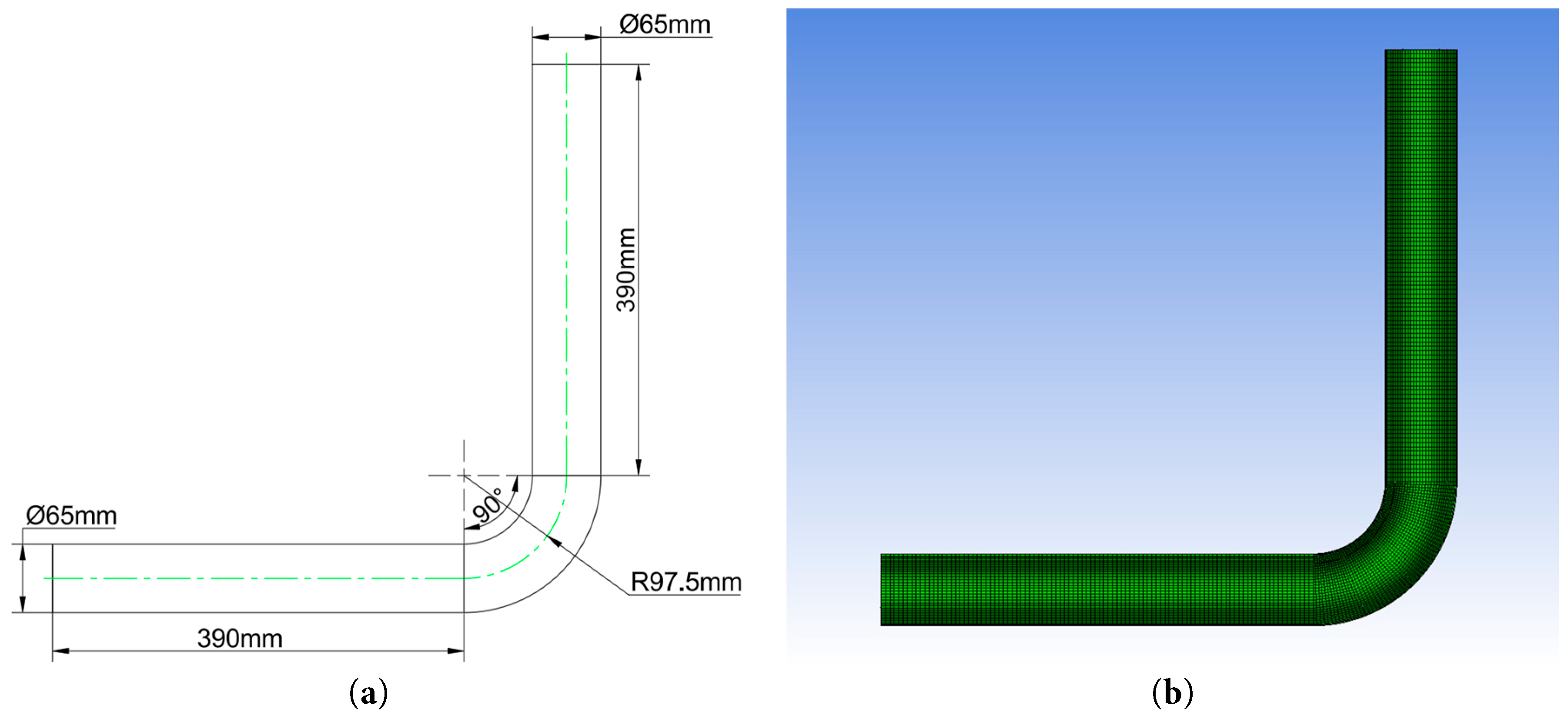
Figure 1: Schematic diagram of the elbow: (a) The geometric dimensions of the elbow; (b) The overall meshes of the elbow.
The gate valve, under the fully open condition, has the following main geometric parameters: nominal diameter 65 mm, and total body length 260 mm. The total length of the extension sections is 780 mm. Under the fully open condition, the resistance coefficient of the gate valve measured in the manufacturer’s factory test with water as the working fluid is 0.17. Local mesh refinement was applied to the central throttling region of the valve, where flow contraction and expansion are most pronounced. The geometric dimensions and the resulting mesh distribution is shown in Fig. 2.
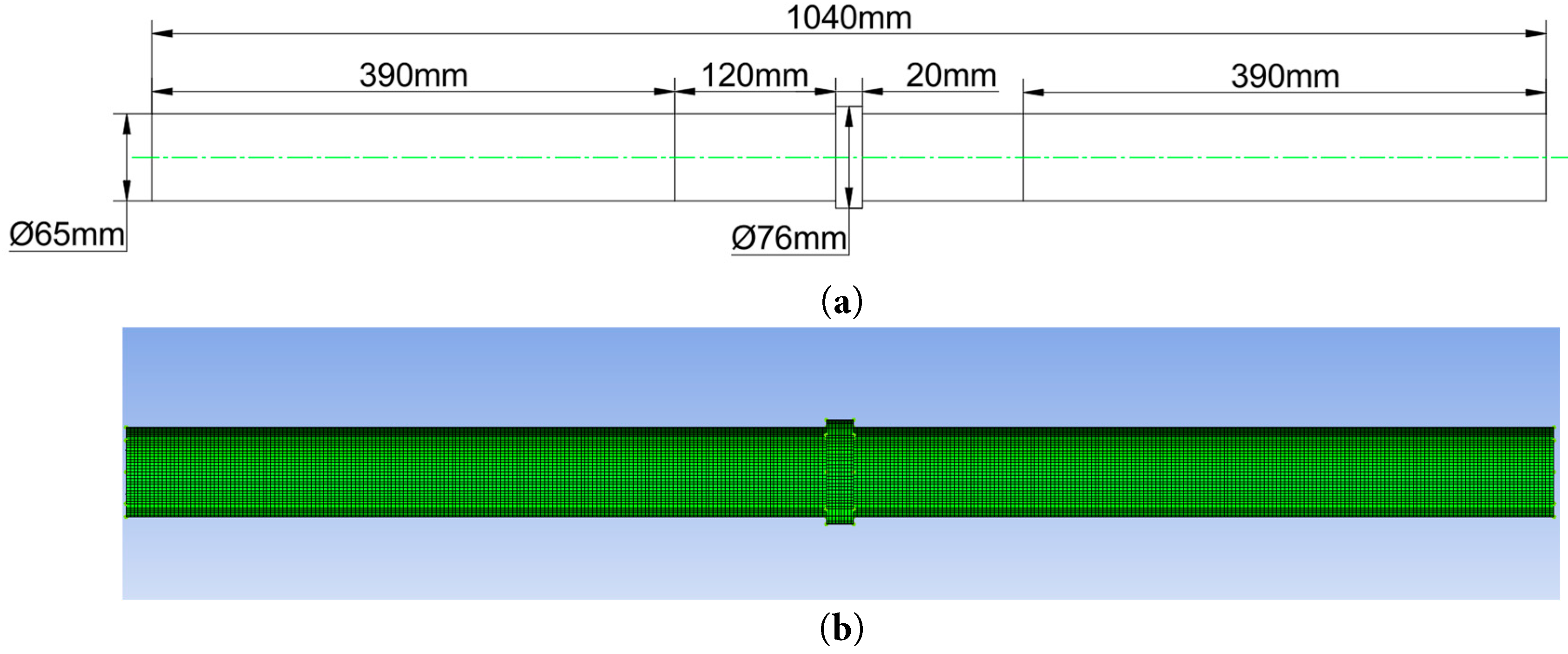
Figure 2: Schematic diagram of the gate valve: (a) The geometric dimensions of the gate valve; (b) The overall meshes of the gate valve.
Since the pressure drop across the gate valve was relatively small compared to the inlet operating pressure, the pressure contours showed minimal variation under standard conditions. An operating pressure of 0.39 MPa was specified in the simulations to enhance the visualization of pressure gradients within the flow domain.
The globe valve model included extension sections with an inner diameter of 65 mm and a total length of 780 mm. The central flow passage was simplified as a 44 mm circular pipe with a total horizontal length of 260 mm, bent to represent the internal flow path of the valve. The junctions between the valve inlet/outlet and the extension sections were modeled with a 45° bend and a curvature radius of 65 mm, while the central flow passage featured a 135° bend with a curvature radius of 31.02 mm. Under the fully open condition, the local resistance coefficient of the globe valve measured in the manufacturer’s factory test with water is 2.3. To improve accuracy in capturing local flow variations, the mesh in the valve flow passage was refined by a factor of two. The geometric dimensions and the meshes of the globe valve are shown in Fig. 3.
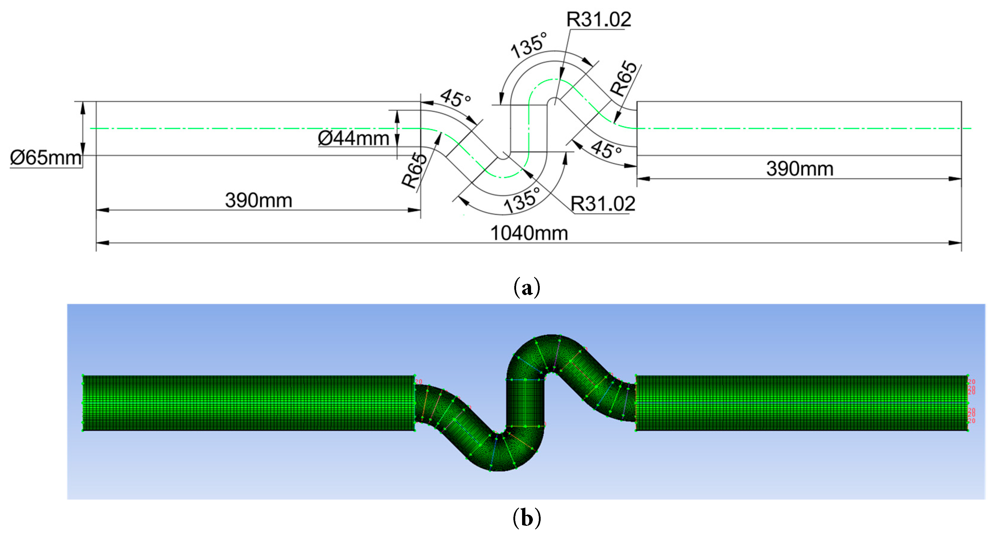
Figure 3: Schematic diagram of the globe valve: (a) The geometric dimensions of the globe valve; (b) The overall meshes of the globe valve.
2.1.4 Gathering and Transportation Interference Simulation of Manifold
The manifold model was established based on real parameters, without extension sections. The inner diameter of the manifold is 100 mm. Each inlet section has a diameter of 65 mm and a length of 350 mm. The inlet sections are numbered sequentially from the end of the manifold toward the outlet as 4#, 5#, 6#, 3#, 2#, and 1#. A local mesh refinement with a density factor of two was applied to the junction regions between each inlet and the main manifold. The geometric dimensions and the meshes of the globe valve are shown in Fig. 4.
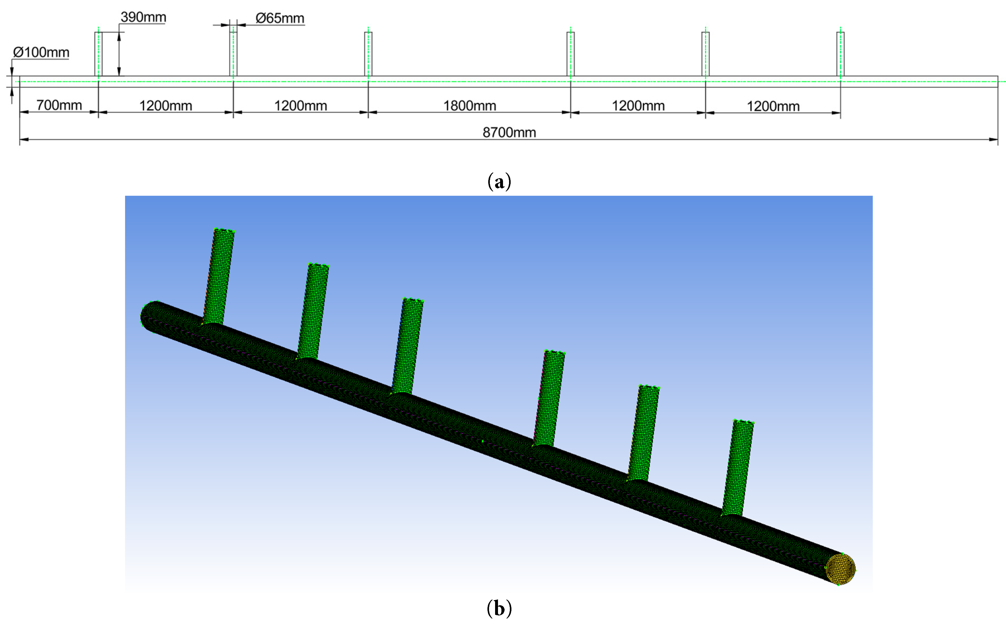
Figure 4: Schematic diagram of the manifold: (a) The geometric dimensions of the manifold; (b) The overall meshes of the manifold.
The high-pressure inlet is designated as 3#. Due to the backflow caused by the interference between high-pressure and low-pressure streams, a pressure inlet and an outflow boundary were defined. A total pressure contour on the manifold cross-section was established to observe the influence of the high-pressure inlet on the pressures at other inlets. Additionally, a cross-sectional velocity vector plot was generated to examine the backflow behavior at the low-pressure inlets. The initial boundary conditions are listed in Table 3.
Table 3: Initial manifold inlet pressures for each group.
| Inlets | Inlet Pressure of Group A (MPa) | Inlet Pressure of Group B (MPa) | Inlet Pressure of Group C (MPa) | Inlet Pressure of Group D (MPa) |
|---|---|---|---|---|
| 1# | 0.4 | 0.4 | 0.4 | 0.4 |
| 2# | 0.4 | 0.4 | 0.4 | 0.4 |
| 3# | 2 | 1 | 0.5 | 0.4 |
| 4# | 0.4 | 0.4 | 0.4 | 0.4 |
| 5# | 0.4 | 0.4 | 0.4 | 0.4 |
| 6# | 0.4 | 0.4 | 0.4 | 0.4 |
2.2 Mesh Independence Verification
Mesh-independence verification for each component was performed based on preliminary steady-state simulations. The geometric models were discretized with several mesh densities and imported into the solver separately. The pressure difference between the inlet and outlet boundaries was used as the monitoring variable for evaluating the pressure drop, and the simulated pressure drop values were recorded for each mesh density. The results are shown in Fig. 5.
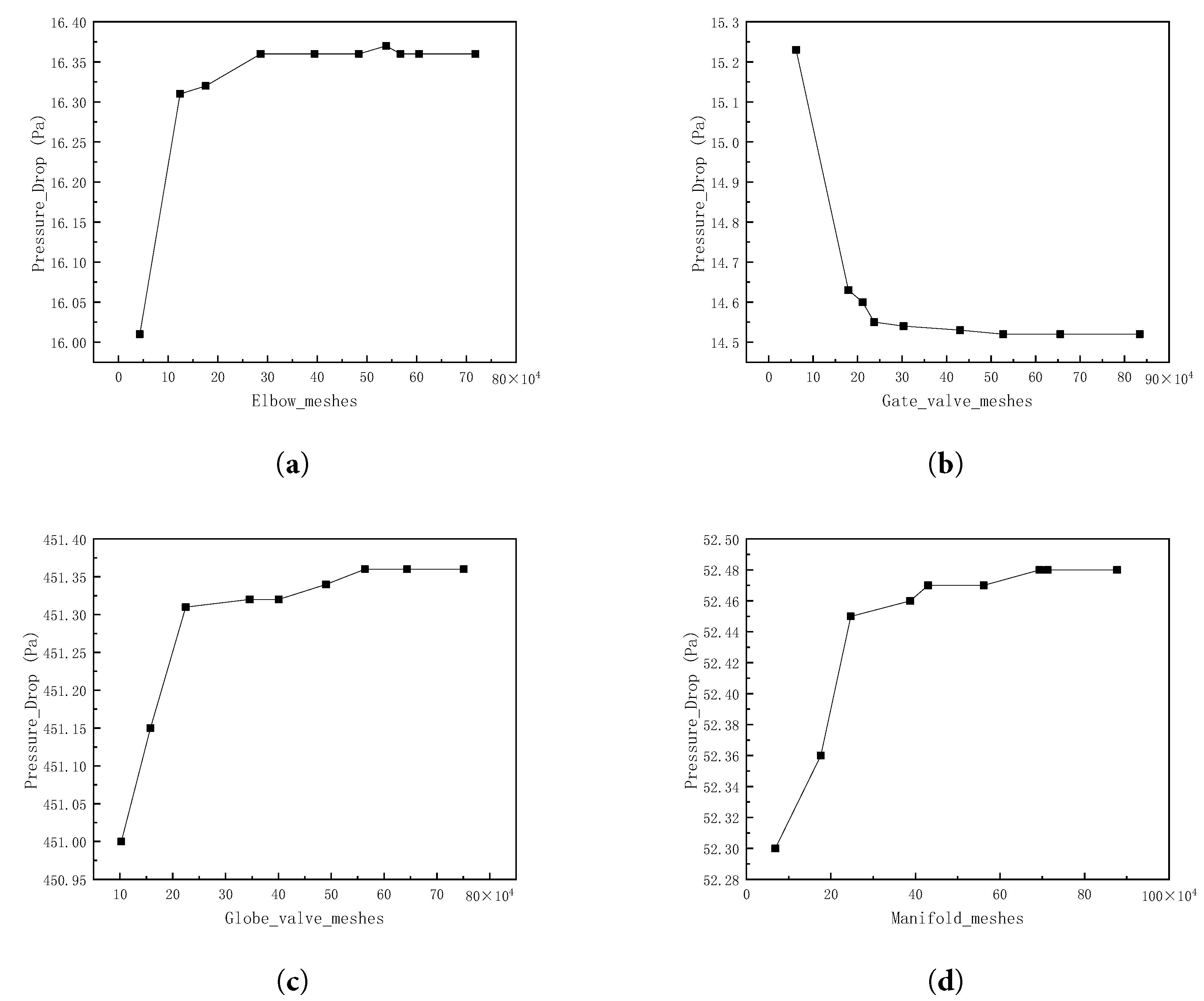
Figure 5: Pressure drop variation of each component with increasing mesh density: (a) Result of elbow; (b) Result of gate valve; (c) Result of globe valve; (d) Result of manifold.
The results show that, when the mesh count of the elbow exceeds 567,360 cells, the predicted pressure drop stabilizes at approximately 16.36 Pa. For the gate valve, the pressure drop becomes stable at around 14.52 Pa once the mesh count exceeds 527,076 cells. For the globe valve, a stable pressure drop of approximately 451.36 Pa is obtained when the mesh count exceeds 643,721 cells. For the manifold, the predicted pressure drop stabilizes near 52.48 Pa when the mesh count is greater than 712,468 cells. Therefore, the final mesh sizes adopted for the production simulations are 567,360, 527,076, 643,721, and 712,468 cells, respectively.
2.3 PipeSim Simulation of Platform Gathering Process
The target shale gas production platform includes six wells. Wells 1#, 2#, and 3# are situated farther from the process area, while Wells 4#, 5#, and 6# are located closer to it. Each well delivers gas to the process area through a gathering pipeline. At the process area inlet, two DN100 manifolds are installed to balance the pressure differences among the wells and ensure stable gas transmission. Within the station, two sets of horizontal separators are deployed. The connection layout of the infield pipelines linking the well area and the process area is shown in Fig. 6.
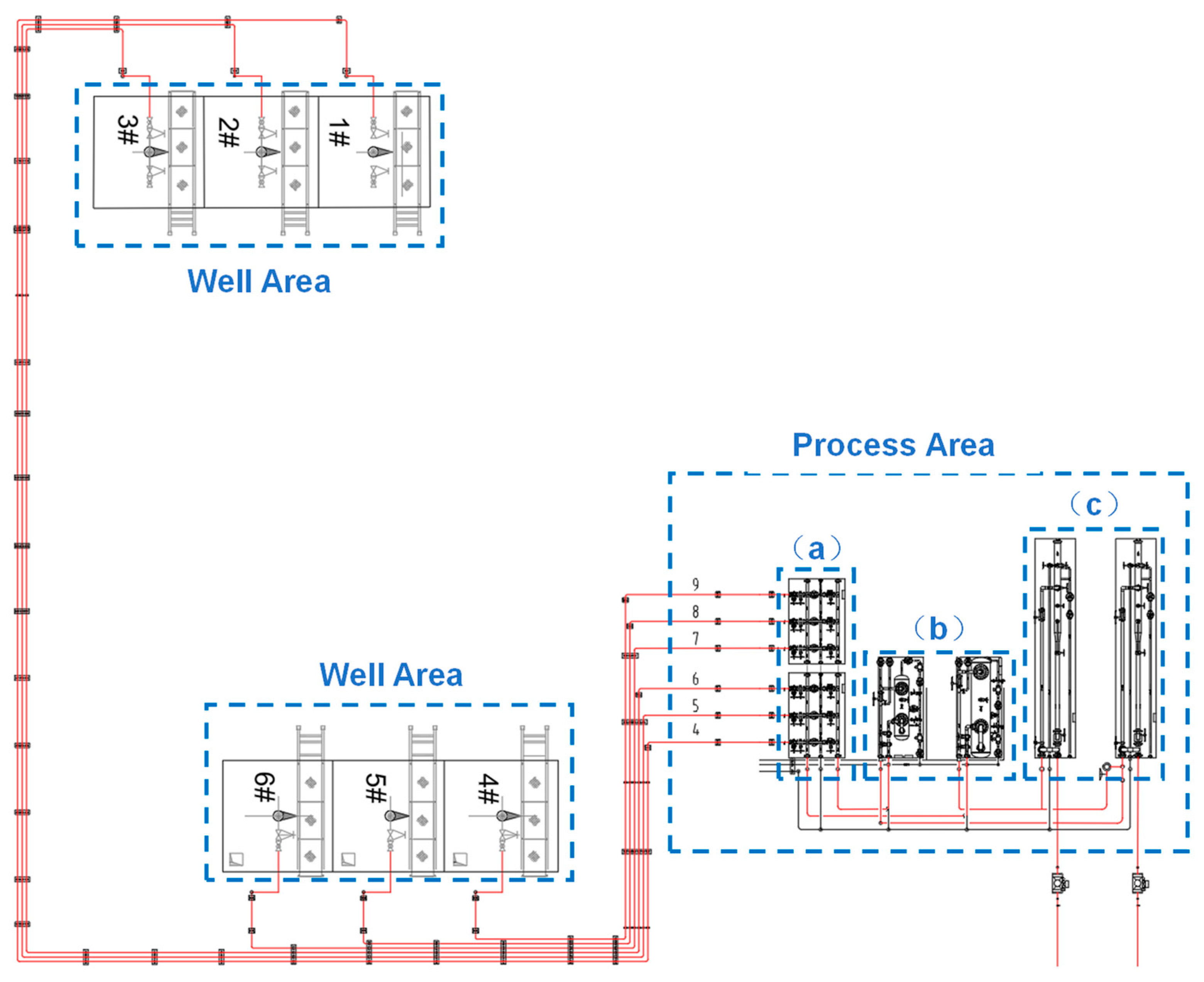
Figure 6: Pipeline flow of the platform: (a) Metering valves; (b) Separators; (c) Pig launcher and receiver.
2.3.1 In-Station Gathering Process Modeling
The station process simulation was conducted using Schlumberger’s PipeSim software. The on-site pipeline routing and layout were reproduced in the model to ensure high fidelity to field conditions. Because the built-in fittings library in PipeSim did not fully meet the actual equipment requirements, the fittings plugin was used to assist model construction; this plugin defines fittings by nominal diameter and parameters such as local loss coefficients. The modeled topology of the in-station gathering network in PipeSim is shown in Fig. 7.
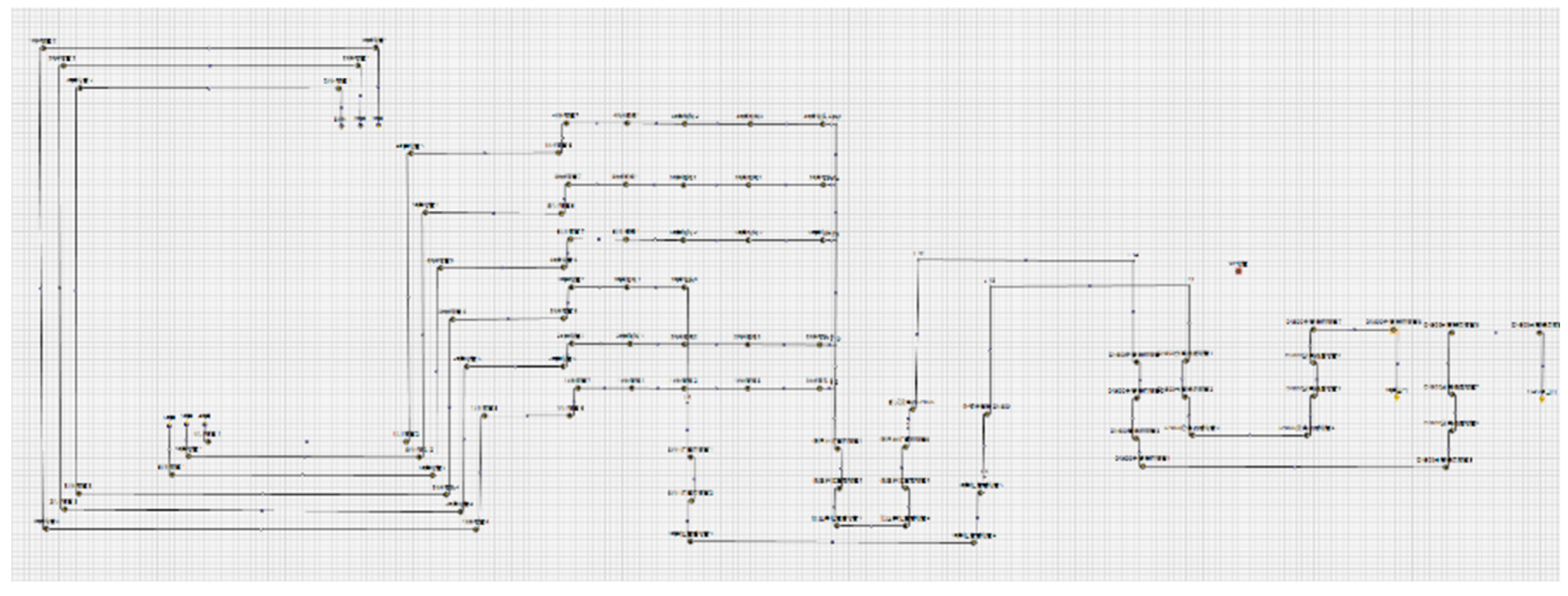
Figure 7: PipeSim model of in-station process.
The platform employs two parallel gathering systems for low-pressure and high-pressure streams. Wells 1#, 2#, 3#, 5#, and 6# are routed into the low-pressure gathering system, while Well 3# is gathered separately via the high-pressure system to reduce the risk of interference that could prevent low-pressure wells from exporting gas.
2.3.2 In-Station Pressure Drop Simulation
SCADA data of the platform were used for the simulation. Four monitoring instants were selected and listed as Table 4:
Table 4: Production data of 04–05 July 2024 of platform H11.
| Wells | Casing Pressure (MPa) | Tubing Pressure (MPa) | Pressure after Throttling (MPa) | Gas Production (104 m3/d) | Water Production (m3/d) | Remarks |
|---|---|---|---|---|---|---|
| 1# | 1.06 | 0.38 | 0.39 | 0.6107 | 0 | Pure gas* |
| 1.25 | 1.27 | 0.13 | 0 | 0 | Shut-in1 | |
| 1.15 | 0.41 | 0.42 | 0.456 | 7.6419 | With water2 | |
| 1.38 | 1.4 | 0.52 | 0 | 0 | Shut-in | |
| 2# | 1.25 | 1.29 | 0.38 | 0 | 0 | Shut-in |
| 1.55 | 1.64 | 0.15 | 0 | 0 | Shut-in | |
| 1.2 | 1.28 | 0.39 | 0 | 0 | Shut-in | |
| 1.62 | 1.69 | 0.52 | 0 | 0 | Shut-in | |
| 3# | 4.48 | 2.03 | 2.03 | 3.9934 | 1.2381 | With water |
| 4.07 | 1.55 | 1.53 | 3.4744 | 0 | Pure gas | |
| 4.55 | 2.09 | 2.08 | 4.0986 | 0 | Pure gas | |
| 4.33 | 1.93 | 1.92 | 3.5721 | 1.0707 | With water | |
| 4# | 2.5 | 2.63 | 0.4 | 0 | 0 | Shut-in |
| 3.06 | 3.06 | 0.15 | 0 | 0 | Shut-in | |
| 2.65 | 2.64 | 0.4 | 0 | 0 | Shut-in | |
| 2.19 | 0.94 | 0.2 | 0 | 0 | Shut-in | |
| 5# | 1.33 | 0.46 | 0.4 | 1.0974 | 3.6997 | High water3 |
| 1.31 | 0.21 | 0.14 | 0.7821 | 2.9528 | High water | |
| 1.35 | 0.45 | 0.39 | 0.7015 | 0.4646 | With water | |
| 1.35 | 0.59 | 0.53 | 0.9152 | 0.5225 | With water | |
| 6# | 0.92 | 0.37 | 0.41 | 0.3014 | 0 | Pure gas |
| 1 | 0.12 | 0.17 | 0 | 0 | Shut-in | |
| 0.96 | 0.4 | 0.43 | 0.5916 | 0 | Pure gas | |
| 1.03 | 0.52 | 0.55 | 0 | 0 | Shut-in |
In the pipeline-network simulations, the data marked as shut-in was excluded and the local resistance coefficients of all fittings were set to their simulated values. Pure methane was used as the gaseous medium and pure water as the liquid phase. The liquid-to-gas ratios and inlet flow conditions were assigned according to the measured data at the corresponding inlet locations. The simulation temperature was set to 300 K.
2.3.3 Pipeline Blockage Approximation
The pipeline segments between each wellhead and the desander inlet is relatively prone to blockage. Due to the absence of desander in the station under analysis, it is reasonable to assume that blockages may occur in the segments between Well Area and Process Area shown in Fig. 6. These segments are characterized by smaller diameters and longer lengths. By reducing the pipe diameters of certain segments within the simulated network, the excessive pressure drop caused by blockage can be effectively represented. This approach allows the simulated network to be calibrated to better match actual operating conditions, thereby providing a basis for analyses of real pipeline parameters.
It should be noted that this treatment is based on steady-state simulations and does not account for transient flow behavior. In addition, a constant flow rate is assumed, and variations in gas well productivity are not considered. Therefore, it can only be used to fit the in-station pressure drop at an apparent level and cannot accurately reflect the actual blockage mechanisms or conditions within the pipelines. Its primary purpose is to enable rapid and approximate assessment of the urgency of maintenance operations through a simplified calculation process, thereby providing preliminary guidance for inspection and repair.
2.3.4 Pressure Drop Simulation with Production Enhancement
Taking the data at the time when each well’s corrected simulation error is minimized as the initial simulation condition, one well’s production rate is increased while keeping the others constant. Each well’s production rate is successively increased by 10%, 20%, 30%, and 40% and the corresponding pressure drops are recorded. For the low-pressure gas wells, on-site operations often involve adjusting the internal process of the station—such as applying platform-wide compression or individual well boosting—to lower the wellhead pressure and thereby enhance single-well productivity. However, when gas wells operate with varying degrees of production enhancement, differing levels of pressure losses occur. Using the corrected simulation pipeline network, the required outlet (post-compression) pressure for each well under different production enhancement levels can be analyzed, providing a basis for determining compressor operating parameters.
3.1 Simulation Results Analysis of Fittings
3.1.1 Local Resistance Coefficient of 90° Elbow
The simulation result of the pressure field is presented in Fig. 8.
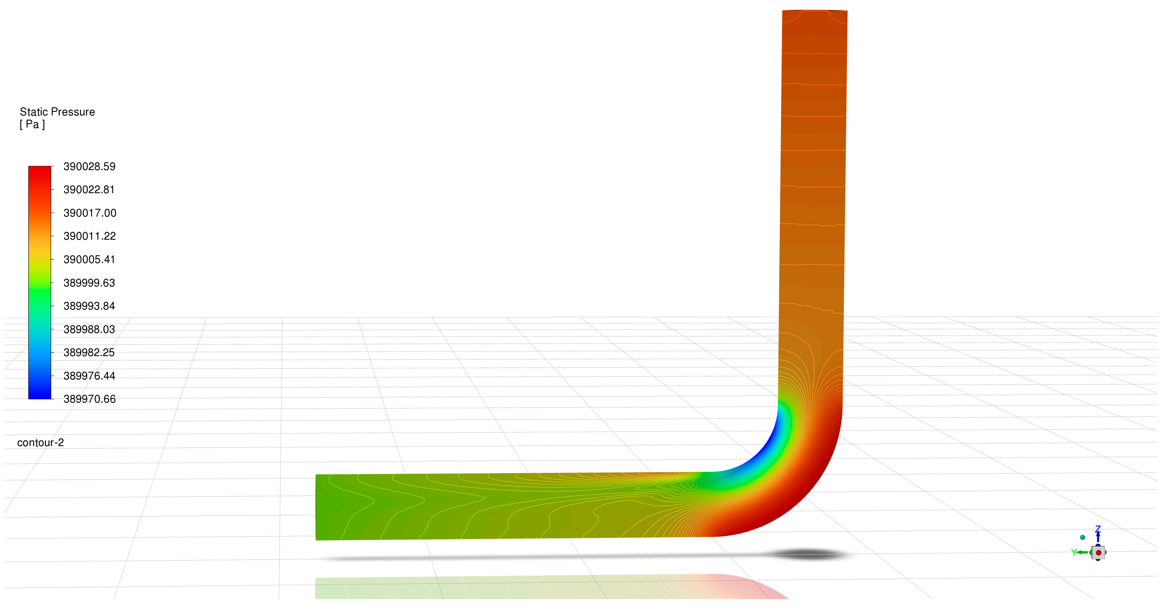
Figure 8: Relative pressure contour of the elbow cross-section.
According to the simulation results, the total pressure drop across the elbow was 16.41 Pa. Based on the calculation using the Eqs. (16) and (19), the pressure loss caused by the inlet and outlet extension sections was 8.56 Pa, resulting in a net pressure drop of 7.85 Pa attributed to the elbow itself. By applying the corresponding equations: Eqs. (9) and (10), the local resistance coefficient of the elbow was determined to be 0.21, and the equivalent length was 0.73 m.
To validate the reliability of the CFD results, the local loss coefficients of the elbow were evaluated using the Ito method and the Darby–3K empirical correlation, and the results were compared with that obtained from the simulation. The Ito method, using Eqs. (11) and (12) for a 90° elbow with R = 1.5 d, gives a reference value of ζE = 0.234. The relative error between the simulated and theoretical values is −10.3%; the Darby-3K method gives a reference value using Eq. (13) is 0.197, and the relative error is 6.6%, suggest that the simulation accuracy is basically satisfactory.
The generation of errors is due to two aspects: The walls of modern equipment are smoother than those used in experiments; and the calculation of the fitting formula also has deviations from the actual situation. Therefore, the error of the simulation results is within the acceptable range.
3.1.2 Local Resistance Coefficient of Gate Valve
The simulation result of the pressure field is presented in Fig. 9.
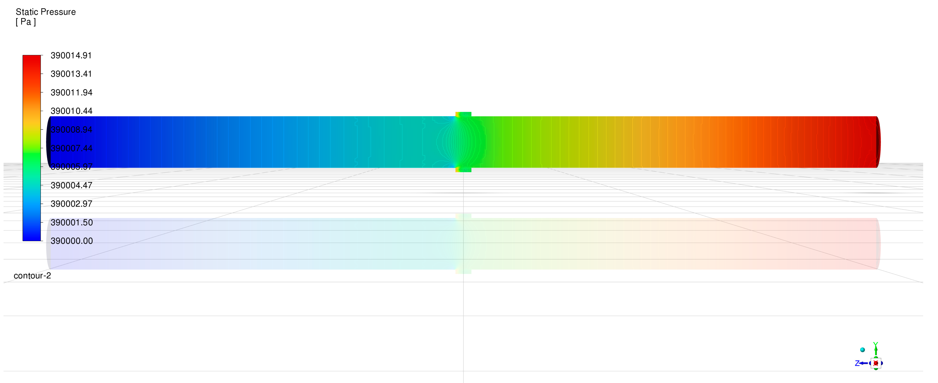
Figure 9: Relative pressure contour of the gate valve cross-section.
The simulated pressure drop across the gate valve was 14.52 Pa. The frictional pressure loss along the inlet and outlet extension sections under the same operating conditions was 8.56 Pa using Eq. (16). Therefore, the total pressure loss within the valve was 5.96 Pa calculated using Eq. (19). The corresponding local resistance coefficient of the gate valve flow passage, calculated using Eq. (9), was 0.16, the equivalent length of the gate valve is 0.54 m, calculated using Eq. (10). Compared with the manufacturer’s factory test value of 0.175, the calculated relative error is −5.88%.
The main source of the error is that, to better reflect actual field conditions, methane (gas) was used as the working fluid in the CFD simulations, whereas water (liquid) was used in the manufacturer’s factory tests. Considering that, the resulting error is acceptable for in-station process modeling.
3.1.3 Local Resistance Coefficient of Globe Valve
The simulation result of the pressure field is presented in Fig. 10.
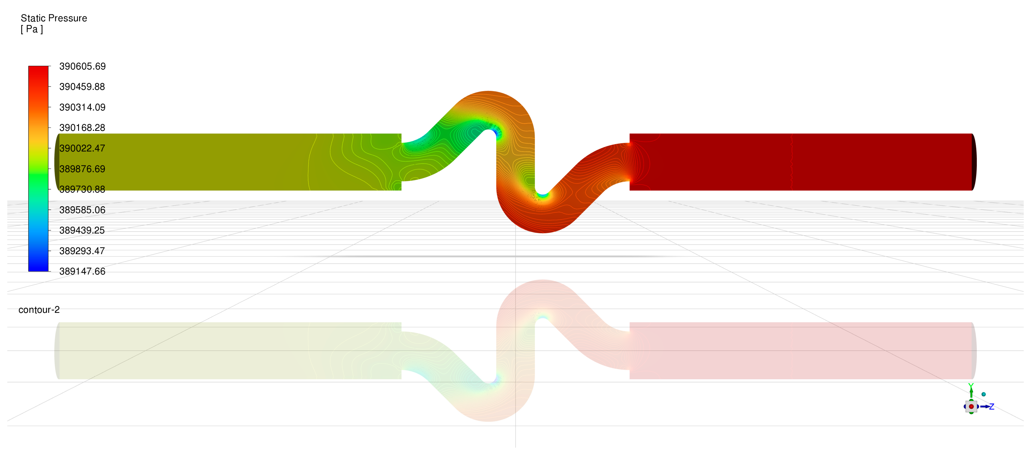
Figure 10: Total pressure contour of the globe valve cross-section.
The simulated pressure drop of the globe valve is 451.36 Pa. According to Eq. (16), the pressure loss caused by the inlet and outlet extension sections under the corresponding operating conditions is 8.56 Pa. The local pressure losses due to the sudden contraction and sudden expansion of the circular pipe, calculated from Eqs. (14) and (15), are 53.60 Pa and 41.55 Pa, respectively. The pressure drop caused by the main flow passage of the globe valve is 347.65 Pa based on Eq. (9), the local resistance coefficient of the flow passage is calculated to be 1.90. The equivalent length of the globe valve is 4.45 m, calculated using Eq. (10). Compared with the manufacturer’s factory test value of 2.3, the calculated relative error is −17.4%.
The calculated results indicate that the simulation error for the globe valve is relatively large. This is mainly because the model adopted in the CFD simulations differs significantly from the actual flow-passage geometry of the globe valve. In the CFD model, the internal flow passage is approximated as a circular pipe, which reduces the pressure losses caused by local vortices compared with the real valve. In addition, the difference between the working fluid used in the factory tests and that adopted in the CFD simulations also contributes to the discrepancy. Owing to the relatively large simulation error, the factory test value of 2.3 is adopted as the local resistance coefficient of the globe valve in the subsequent PipeSim in-station process modeling.
3.2 Interference Mechanism Analysis of Manifold
3.2.1 Simulation Results Analysis of High-Pressure Inlet at 2 MPa
The simulated pressure field of the manifold when the pressure of 3# inlet is 2 MPa is shown in the Fig. 11.
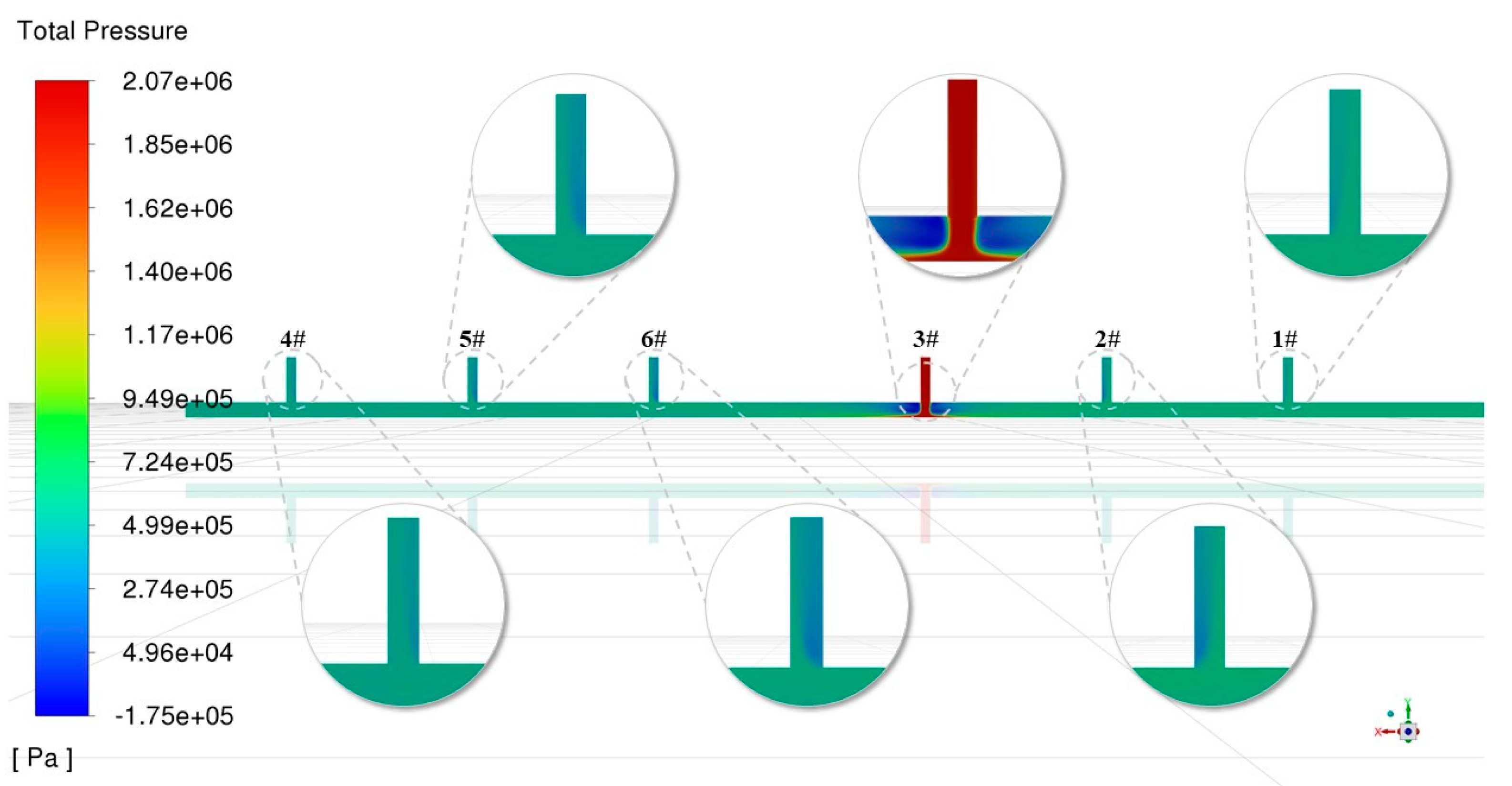
Figure 11: Total pressure contour of the overall cross section for 3# Inlet at 2 MPa.
The right side of the overall cross section corresponds to the outlet of the manifold in Fig. 11. When the inlet pressure of 3# is 2 MPa, the total pressure contour of the manifold shows a clearly defined high-pressure region near the 3# inlet. Other inlets exhibit localized high-pressure zones of varying magnitudes, while the pressure in the main body of the manifold remains generally uniform. Taking the 2# inlet as an example, the left side—adjacent to the 3# high-pressure inlet—corresponds to a low-pressure zone, whereas the right side—closer to the manifold outlet—shows a high-pressure region. The corresponding local velocity vector variations at each inlet are shown in Fig. 12.

Figure 12: Velocity vector distribution at each inlet for 3# Inlet pressure of 2 MPa.
The local velocity vector diagrams at each inlet indicate that when the monitored pressure at the low-pressure inlet sections exceeds 0.4 MPa, the flow behavior changes significantly. On the side close to the high-pressure inlet, the velocity vectors initially point from the inlet toward the manifold, but then swirl at the junction and reverse direction, forming a backflow zone. On the side farther from the high-pressure inlet, a pure backflow region appears, with flow entirely directed from the manifold toward the inlet.
When the inlet region is divided by the swirling zone boundary, the pure backflow region corresponds to the high-pressure area in the total pressure contour, while the inflow–swirl–backflow transition region corresponds to the low-pressure area. As the distance between the inlet and the high-pressure inlet increases, the proportion of the pure backflow (high-pressure) region gradually expands. For instance, Inlet 4#, which is farthest from the high-pressure inlet, exhibits complete backflow according to both the velocity vector and total pressure contours, indicating that gas cannot enter the manifold through this inlet. In summary, when the high-pressure inlet pressure remains constant, backflow occurs at other inlets once their average sectional pressure exceeds 0.4 MPa. The backflow intensity increases with both the pressure difference from the 0.4 MPa threshold and the distance from the high-pressure inlet.
3.2.2 Simulation Results Analysis of High-Pressure Inlet at 1.5 MPa, 0.5 MPa and 0.4 MPa
The simulated pressure field of the manifold when the pressure of 3# inlet is 1.5 MPa, 0.5 MPa and 0.4 MPa is shown in Fig. 13. The pressure variation of each inlet with that of high-pressure inlet is shown in Fig. 14.
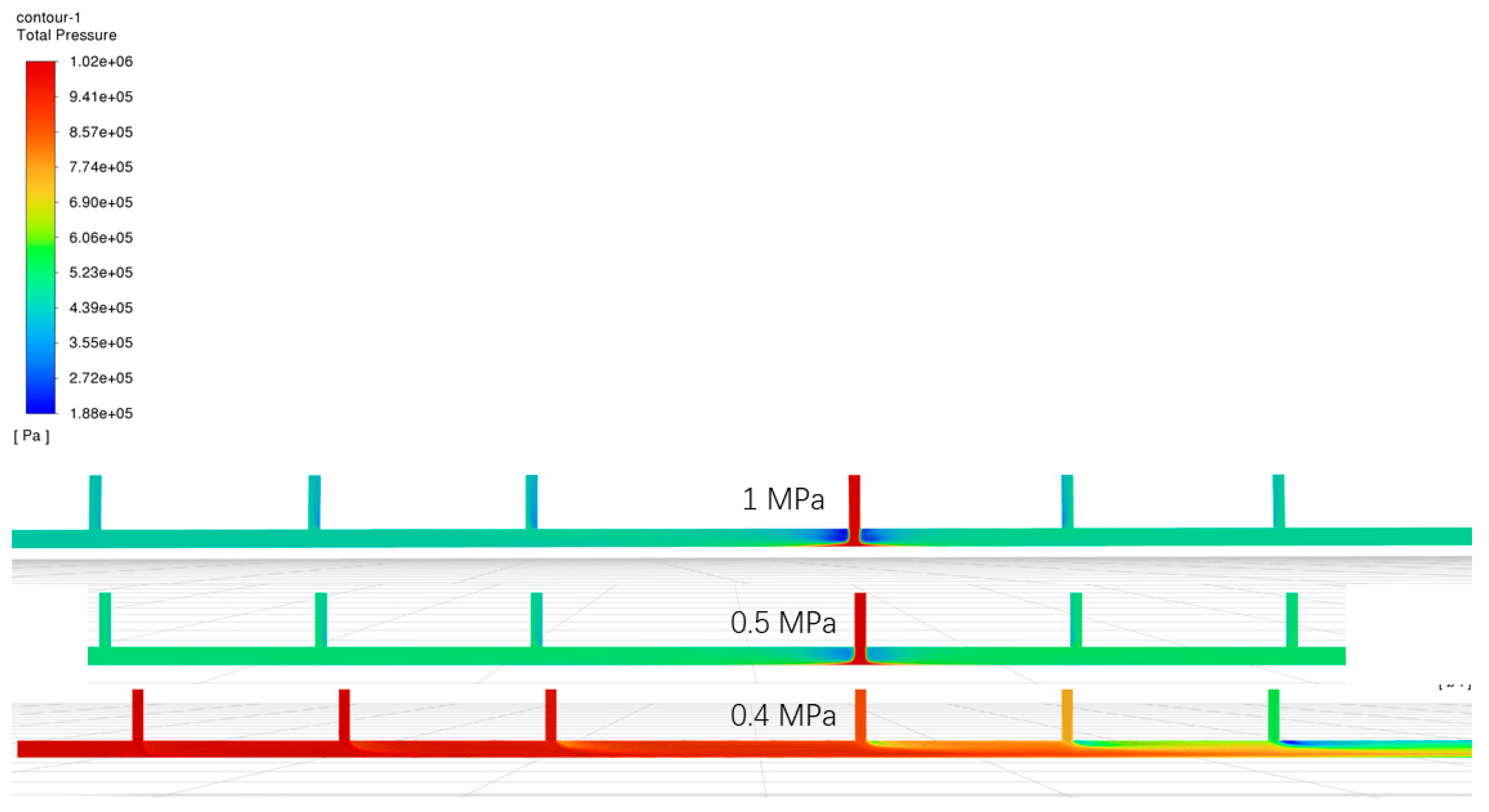
Figure 13: Total pressure contours of the overall cross section for 3# Inlet at 1 MPa, 0.5 MPa, and 0.4 MPa.

Figure 14: Variation curves of average total pressure at each inlet with 3# Inlet pressure.
The simulation results indicate that as the pressure at the high-pressure inlet decreases, the overall pressure within the manifold and the average total pressure at other inlets both decline, exhibiting an approximately linear relationship. This trend suggests that the backflow intensity at the other inlets weakens and the degree of interference from the high-pressure inlet gradually diminishes.
For the inlets located on the same side as the high-pressure inlet (Inlets 4#, 5#, and 6#), the average pressure increases with the distance from the high-pressure inlet. A similar pattern is observed on the opposite side (Inlets 1# and 2#); however, the average pressures of Inlets 1# and 2#—situated closer to the manifold outlet—are overall higher than those on the opposite side. This indicates that when the inlets are distributed on both sides of the high-pressure inlet, the side closer to the manifold outlet experiences stronger interference from the high-pressure inlet.
3.3 Simulation Results Analysis of Platform Gathering Process
3.3.1 Simulation Results of Pressure Drop within Platform
When the simulated pressure drop is greater than the measured value, the error is recorded as positive; when the simulated pressure drop is smaller than the measured value, the error is recorded as negative. The results are shown in Table 5. Based on the simulation results obtained from PipeSim, it is observed that the simulated pressure drops for Wells 1#, 3#, 5#, and 6# are consistently lower than the actual measured values, with the error range remaining relatively stable. This suggests that the gathering pipeline network within the station for these wells likely experiences abnormal increases in pressure loss, possibly caused by partial blockage, internal scaling, or damage of fittings within certain sections of the pipeline.
In a comparable production block operating under similar conditions, a similar issue was reported where the simulated station pressure drop was significantly lower than the field-measured value. Subsequent on-site inspection revealed that portions of the pipelines were severely blocked. The field-observed blockage status is shown in Fig. 15.
Table 5: Comparison between real and simulated pressure drops.
| Wells | Date | Pressure after Throttling (MPa) | Inlet Pressure of Compressor (MPa) | Real Pressure Drop (MPa) | Simulated Pressure Drop (MPa) | Relative Error (%) |
|---|---|---|---|---|---|---|
| 1# | 2024-7-4 9:00:00 | 0.39 | 0.36 | 0.03 | 0.0094 | −68.66 |
| 3# | 2024-7-4 9:00:00 | 2.03 | 1.95 | 0.08 | 0.0211 | −73.6 |
| 3# | 2024-7-4 15:00:00 | 1.53 | 1.47 | 0.06 | 0.0134 | −77.67 |
| 3# | 2024-7-5 9:00:00 | 2.08 | 2.01 | 0.07 | 0.0134 | −80.86 |
| 3# | 2024-7-5 15:00:00 | 1.92 | 1.85 | 0.07 | 0.0111 | −84.08 |
| 5# | 2024-7-4 9:00:00 | 0.4 | 0.36 | 0.04 | 0.0124 | −68.89 |
| 5# | 2024-7-5 9:00:00 | 0.39 | 0.37 | 0.02 | 0.00648 | −67.62 |
| 5# | 2024-7-5 15:00:00 | 0.53 | 0.49 | 0.04 | 0.00449 | −88.78 |
| 6# | 2024-7-4 9:00:00 | 0.41 | 0.36 | 0.05 | 0.00786 | −84.27 |
| 6# | 2024-7-5 9:00:00 | 0.43 | 0.37 | 0.06 | 0.00453 | −92.45 |

Figure 15: Blockage of partial pipeline and fitting.
The figure illustrates two different blockage patterns. In this study, the blockage simulated by reducing the pipe diameter corresponds to the pattern shown on the left, where deposits uniformly cover the inner wall of the pipe, resulting in an effective uniform reduction in the inner diameter. However, blockage morphologies can vary significantly among different stations due to differences in gas composition and operating conditions. When a large discrepancy is observed between the pressure drops predicted by this method and the measured values, it indicates that the actual pipeline blockage at the station exhibits strong non-uniformity, the proposed approach loses its capability for quantitative assessment.
When pipeline blockage occurs, the effective flow cross-sectional area may be reduced to less than half of its initial value, which not only affects gathering and transportation efficiency but also results in an extremely high pressure drop along the pipeline. Therefore, the subsequent pipeline network parameter correction is based on the assumption of pipeline blockage.
3.3.2 Approximate Calculation of Pipeline Blockage Degree
By adjusting the pipeline inner diameter to fit the in-station pressure drop, the simulation results for wells 1#, 5#, and 6# are shown in Fig. 16.
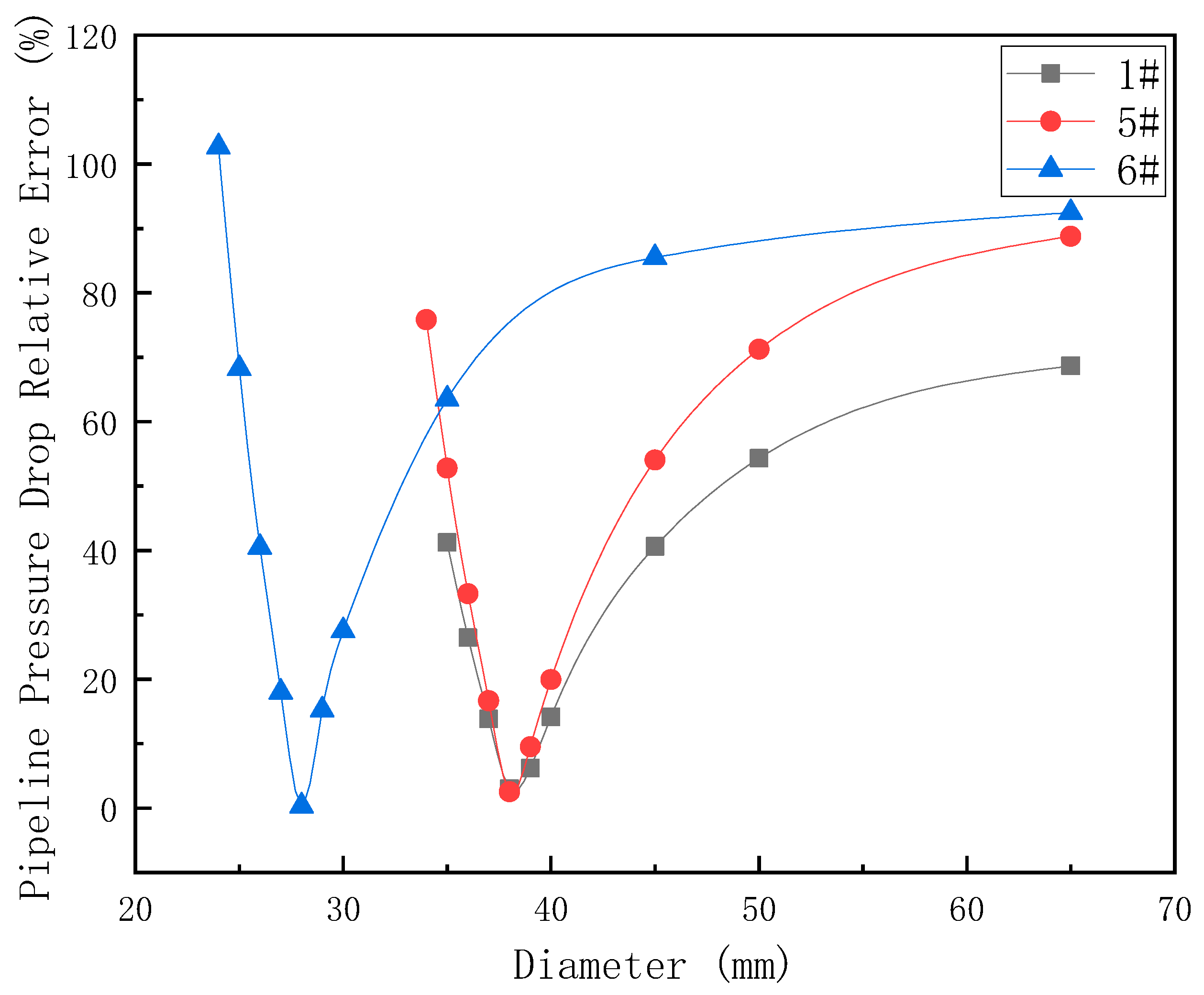
Figure 16: Pressure drop error curves under varying pipeline diameters of Wells 1#, 5#, and 6#.
The vertical axis represents the absolute value of the error. As the pipeline diameter decreases, the absolute error for each pipeline first decreases and then increases overall. The minimum errors for Wells 1#, 5#, and 6# correspond to diameters of 38 mm, 38 mm, and 28 mm, with absolute errors of 3.03%, 2.54%, and 0.33%, respectively. Therefore, according to Eq. (17), the calculated blockage degrees of the corresponding pipelines are 65.82%, 65.82%, and 81.44%, respectively.
Three days of production data for Wells 1#, 5#, and 6# were randomly selected from the field-collected production dataset to evaluate the fitting accuracy of the PipeSim-based model. The selected data are listed in Table 6.
Table 6: Wells 1#, 5# and 6# production data for test.
| Groups | Wells | Pressure after Throttling (MPa) | Gas Production (104 m3/d) | Water Production (m3/d) | Measured Pressure Drop (MPa) | Simulated Pressure Drop (MPa) | Relative Error (%) |
|---|---|---|---|---|---|---|---|
| A | 1# | 0.39 | 0.6572 | 0 | 0.03 | 0.03059 | 1.977 |
| 5# | 0.39 | 0.7201 | 0.562 | 0.03 | 0.03138 | 4.586 | |
| 6# | 0.41 | 0.5224 | 0 | 0.05 | 0.05151 | 3.023 | |
| B | 1# | 0.36 | 0.4387 | 0 | 0.02 | 0.01588 | −20.593 |
| 5# | 0.36 | 0.5472 | 0.3258 | 0.02 | 0.01945 | −2.730 | |
| 6# | 0.38 | 0.4406 | 0 | 0.04 | 0.03867 | −3.313 | |
| C | 1# | 0.37 | 0.5719 | 0 | 0.02 | 0.02195 | 9.725 |
| 5# | 0.37 | 0.6348 | 0.3865 | 0.02 | 0.02125 | 6.270 | |
| 6# | 0.36 | 0.2039 | 0 | 0.01 | 0.01123 | 12.251 |
As indicated by the testing errors in the table, the fitted simulation network achieves relatively high accuracy and can generally reproduce the actual on-site pressure drop behavior, making it suitable for subsequent production-increase simulations. However, it is also observed that the error for Group B Well 1# is relatively large, indicating that uniformly reducing the diameter of the pipeline section from the well outlet to the process-area inlet alone cannot fully represent the actual conditions of pipeline blockage or fitting damage in the field. Therefore, this method can only provide a semi-quantitative characterization of on-site faults, and the specific fault locations need to be identified through further field investigations or additional segmented pipeline testing data. The simulated results for the pipeline of Well 3# are shown in Fig. 17.
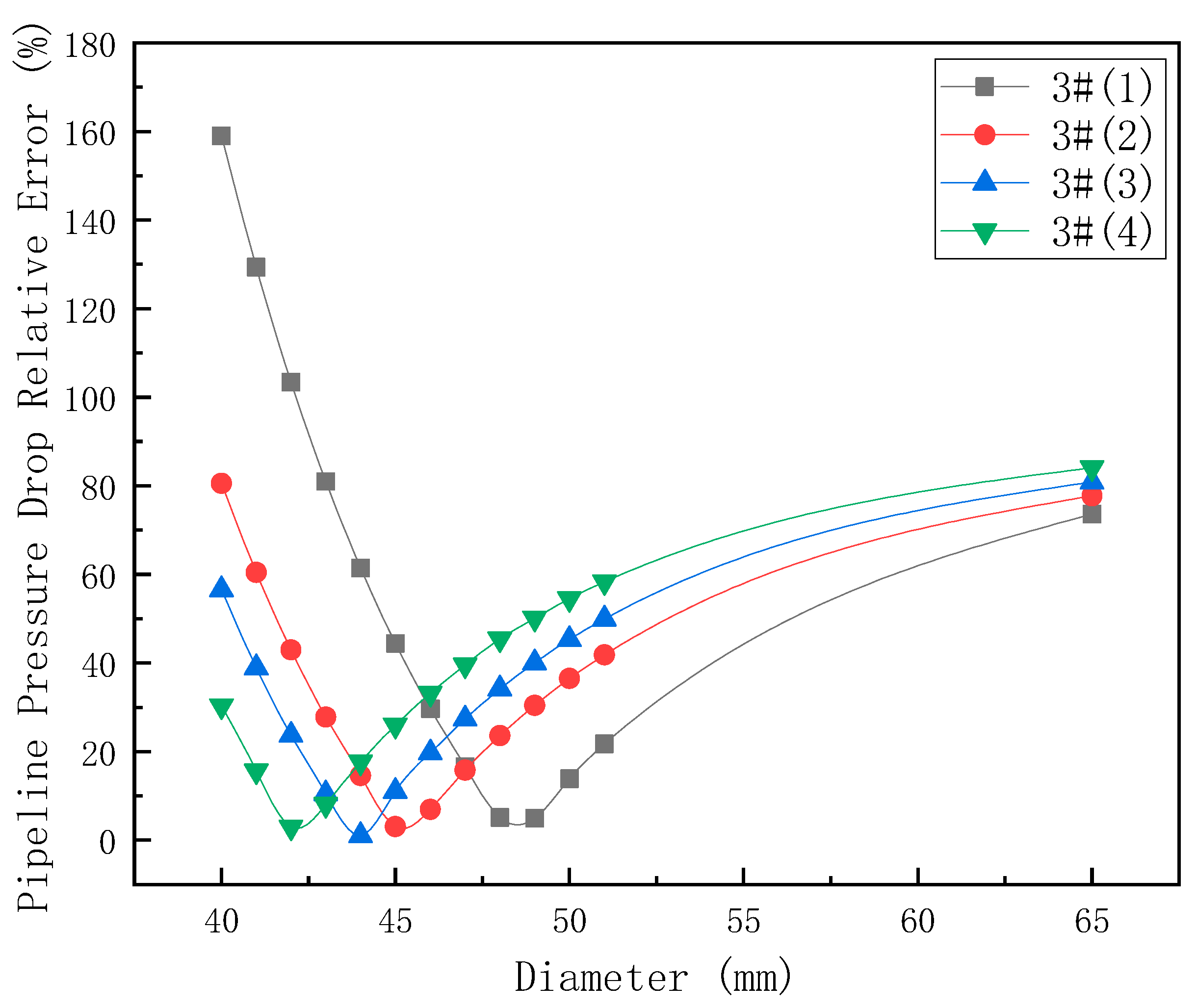
Figure 17: Pressure drop error curves under varying pipeline diameters of well 3#.
The curves correspond to the simulated pressure drop under different initial conditions at four time points: the morning and afternoon of 4th July and 5th July. Curves 1 and 4 represent conditions with water production, resulting in their minimum points deviating more noticeably compared to Curves 2 and 3. Considering the actual operating conditions of Well 3# and the overall error distribution among the curves, the simulated error is relatively small when the pipeline inner diameter is 44 mm. Under this condition, the average absolute error of Curves 2, 3, and 4 is 11.06%, while the absolute error of Curve 3 is 1.01%. According to Eq. (17), the degree of blockage in the pipeline of Well 3# is calculated to be 54.18%. Similar to the accuracy tests for Wells 1#, 5#, and 6#, production data were randomly selected to evaluate the model fitting accuracy for Well 3# after adjusting the pipeline diameter, and the results are presented in Table 7.
Table 7: Well 3# Production data for test.
| Data | Pressure after Throttling (MPa) | Gas Production (104 m3/d) | Water Production (m3/d) | Measured Pressure Drop (MPa) | Simulated Pressure Drop (MPa) | Relative Error (%) |
|---|---|---|---|---|---|---|
| Day1 | 1.87 | 3.5390 | 0 | 0.05 | 0.05426 | 8.528 |
| Day2 | 2.20 | 4.0171 | 1.3029 | 0.13 | 0.11497 | −11.559 |
| Day3 | 1.95 | 3.8125 | 0 | 0.05 | 0.05194 | 3.882 |
The test results for Well 3# show that the accuracy generally meets the requirements; however, the model performs relatively poorly under the water-producing condition on Day 2. This likewise indicates that the pipe-diameter reduction approach can only achieve a partial fit and provides only a semi-quantitative analysis of abnormal operating conditions within the station.
Considering the predefined assumptions of this study (steady flow and steady-state simulations) together with the simulation results, the approach of representing in-station blockage conditions by reducing the effective pipe diameter has inherent limitations: (1) It relies heavily on accurate field-measured data as a reference for calibration and fitting; (2) Since this method cannot capture the actual physical mechanisms of blockage caused by sediments or similar deposits, it is unable to identify the true causes or morphological characteristics of pipeline blockage through non-intrusive analysis; (3) When the flowing medium transitions from dry gas to gas with associated liquid production, the fitting error increases further.
Therefore, this method is most suitable for rapid and simplified assessment of mid to late-stage shale gas gathering stations, where gas production is relatively stable, fluid composition does not vary significantly during the analysis period, and the internal blockage configuration of pipeline segments has already become relatively fixed.
3.3.3 Simulation Result Analysis of Pressure Drop Variation with Production
The results are shown in Table 8 and Fig. 18.
Table 8: Pipeline pressure drop under different production enhancement levels.
| Enhancement Levels (%) | Well 1# Pipeline Pressure Drop (MPa) | Well 3# Pipeline Pressure Drop (MPa) | Well 5# Pipeline Pressure Drop (MPa) | Well 6# Pipeline Pressure Drop (MPa) |
|---|---|---|---|---|
| 0 | 0.0341 | 0.0693 | 0.0438 | 0.067 |
| 10 | 0.0396 | 0.0833 | 0.0525 | 0.083 |
| 20 | 0.0455 | 0.0986 | 0.062 | 0.0969 |
| 30 | 0.0518 | 0.115 | 0.0721 | 0.111 |
| 40 | 0.0585 | 0.133 | 0.0829 | 0.127 |
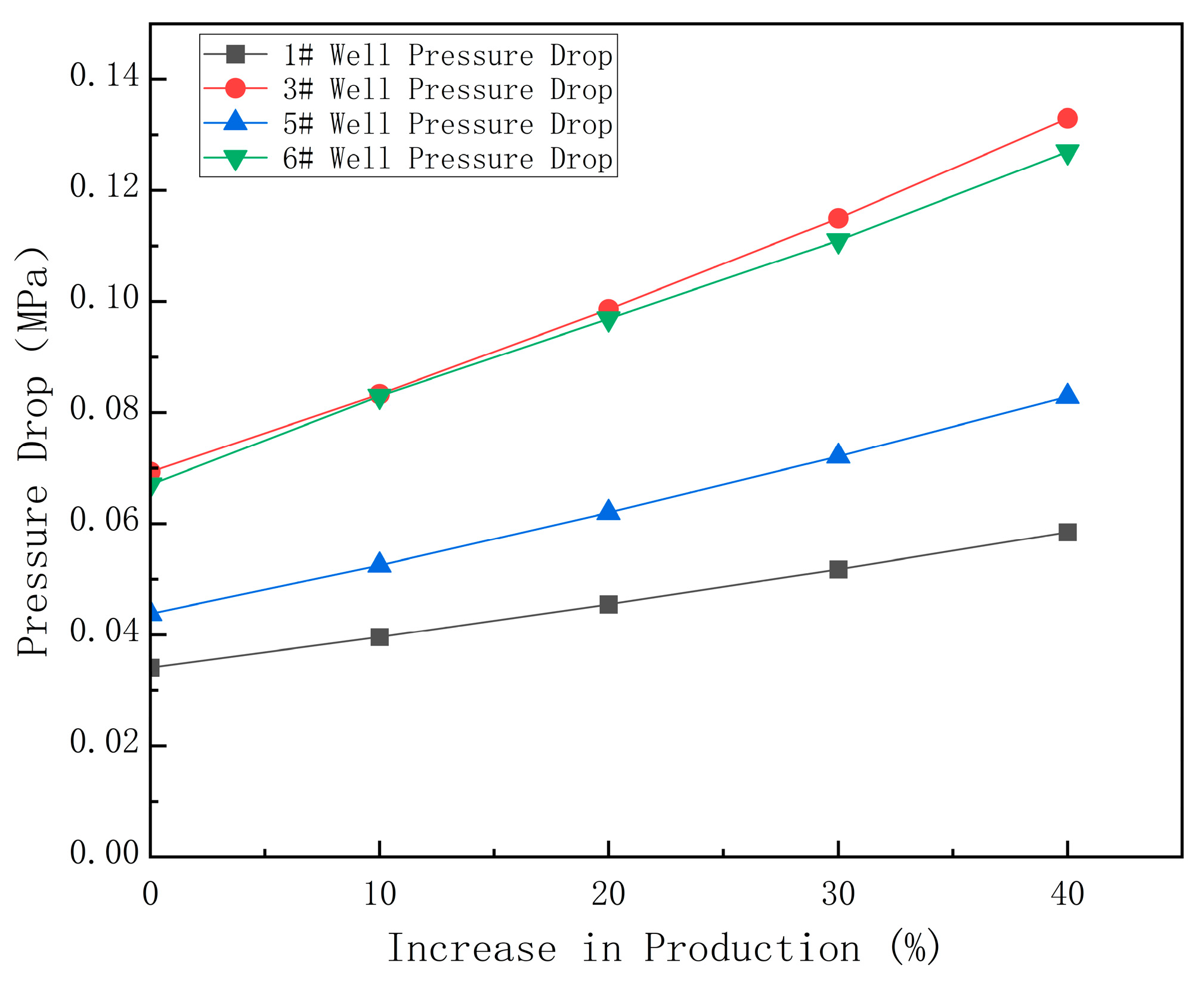
Figure 18: Variation curves of pipeline pressure drop with increasing production rate.
According to the simulation results, the production increase of each well shows an approximately linear relationship with the corresponding pressure drop. Therefore, linear regression can be applied to the above data to obtain pressure-drop–production-increase curves, which can be used to predict pipeline pressure drops under higher production enhancement scenarios. By combining these curves with the gathering pipeline network performance curve (i.e., outlet pressure vs. total platform production), it becomes possible to determine the wellhead pressure at various production enhancement levels for each well. By plotting the wellhead characteristic curve (with wellhead pressure as the solution point), the pipeline network performance curve, and the pressure-drop–production relationship curve on the same graph, the overall production–pressure interaction can be illustrated as shown in Fig. 19.
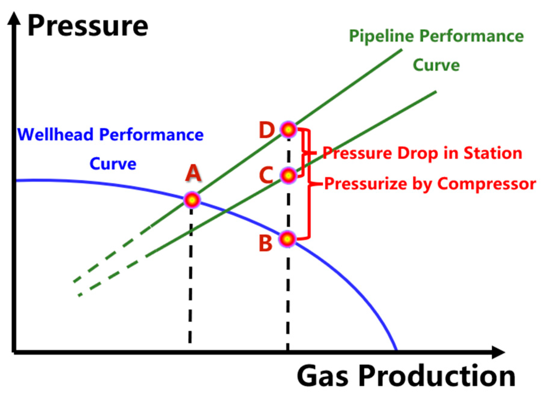
Figure 19: Schematic Diagram for the pressurization and production enhancement capacity.
The wellhead characteristic curve is obtained by fitting the bottom-hole flowing pressure–production rate relationship to derive the inflow performance relationship. Using multiphase flow equations, the pressure drop between the bottom hole and the wellhead can be calculated for different production rates, thereby determining the remaining wellhead pressure under given conditions—this constitutes the wellhead characteristic curve.
Point A represents the maximum coordinated production rate at which the wellhead pressure satisfies the outlet pressure requirement. The curve passing through Point C corresponds to the gathering pipeline network performance curve, which reflects the minimum outlet pressure of the system under different total production rates. The curve passing through Point D represents the individual well’s outlet performance curve, obtained by adding the additional station pressure loss to the pipeline network performance curve.
The pressure difference between Points D and C indicates the incremental station pressure drop resulting from increased production, while the difference between Points D and B represents the required compression pressure that must be supplied by the compressor to achieve the higher production rate. When the compressor’s boosting capacity is fixed, this method allows for determining the maximum producible wellhead pressure that satisfies the gathering system’s requirements, providing valuable guidance for optimizing gas well production strategies.
This study focuses on the H11 platform in a shale gas block. CFD simulations were conducted to analyze fitting pressure losses and the interference of manifold. Corrected local resistance coefficients of fittings were integrated into a PipeSim network model to assess pressure drops under production enhancement scenarios and to determine the maximum production capacity. The main conclusions are as follows:
- 1.By comparing the simulated local resistance coefficients with the recommended empirical values, the corrected coefficients suitable for field conditions are 0.21 for 90° elbows, 0.16 for gate valves, and 2.3 for globe valves. These results indicate that standard empirical values may underestimate local losses in shale gas gathering stations, highlighting the necessity of correction for accurate pressure drop under working conditions.
- 2.Mutual interference of the manifold exists between inlets: As the high-pressure inlet pressure decreases, the interference intensity at other inlets also decreases; When the high-pressure inlet pressure remains constant, inlets further away on the same side experience stronger interference; Inlets closer to the manifold outlet experience stronger interference compared with those near the blind end. These findings provide a basis for optimizing flow distribution within manifolds.
- 3.The PipeSim simulated pressure drops were significantly lower than measured values., It was inferred that partial blockages occurred in the pipelines between the wells and the process area. The pipeline blockage degrees of Well 1#, Well 3#, Well 5#, and Well 6# are equivalent to the inner diameter being reduced from 65 mm to 38 mm, 44 mm, 38 mm, and 28 mm respectively. To a certain extent, this provides a rapid and straightforward quantitative method for evaluating the degree of blockage in pipelines in a shale gas station.
- 4.Based on the corrected network model, the station pressure drop under various production increases was calculated. By combining the wellhead characteristic curve and the gathering network characteristic curve, it is possible to determine: The required compressor boost for a given production enhancement, or the maximum achievable production rate and corresponding wellhead pressure under a fixed compressor capacity.
Further research
Owing to limitations in testing conditions, data availability, and other technical factors, several aspects remain insufficiently addressed and warrant further investigation.
- 1.CFD simulation of flow losses in a globe valve: The flow passage structure of the globe valve is more complex compared to other fittings. Results show that the simplified flow passage structure is insufficient to fully represent the actual situation, leading to significant error.
- 2.The local resistance coefficients of elbows and fully open gate and globe valves obtained in this study using pure methane as the working fluid can only be regarded as reference values under the specified physical conditions. Applying these reference values to in-station network modeling cannot fully reproduce operating conditions in which gas wells produce associated water. To improve the model fidelity, our future work will focus on simulating local resistance coefficients under varying inlet gas–liquid ratios, pressures, and orientations of bends and valves. The core contribution of this study is the proposal of a simple methodology for evaluating in-station pressure losses and blockage conditions, which can serve as a reference for the analysis of stations with similar characteristics.
- 3.The fundamental mechanism behind the interference in the manifold: Due to the lack of experimental conditions, the physical mechanisms of manifold interference have not been investigated through physical experiments. Instead, CFD simulations were used to analyze the phenomenon for field application. Further research could focus on the mechanisms of vortex formation and development, as well as the interference phenomena when different inlet pressures exist simultaneously in the manifold, along with the pressure drop distribution patterns.
- 4.Due to the lack of data from the spot between the well and process areas, an approximate method was used to fit the failure conditions. While the overall fitting accuracy meets requirements, some pipelines show significant errors under certain conditions. It is recommended to perform pressure drop fitting in segments with sufficient data to improve accuracy and enable quantitative analysis of the in-plant pressure drop distribution.
Acknowledgement:
Funding Statement: This research was funded by the National Natural Science Foundation of China under Grant 52441411, 52325402 and 52274057, Deep Earth Probe and Mineral Resources Exploration-National Science and Technology Major Project under Grant 2024ZD1004302-04, the National Key R&D Program of China under Grant 2023YFB4104200.
Author Contributions: The authors confirm contribution to the paper as follows: Conceptualization, Kunyi Wu, Liming Zhang and Hui Li; methodology, Kunyi Wu, Bo lei and Hui Li; software, Bo Lei and Hui Li; validation, Kunyi Wu, Bo Lei, Yanhua Qiu and Shize Wei; formal analysis, Yanhua Qiu; investigation, Yanhua Qiu and Shize Wei; resources, Yu Wu and Liming Zhang; data curation, Shize Wei; writing—original draft preparation, Kunyi Wu, Bo lei and Hui Li; writing—review and editing, Yu Wu and Liming Zhang; visualization, Feng Wang; supervision, Yu Wu and Liming Zhang; project administration, Yu Wu; funding acquisition, Liming Zhang. All authors reviewed and approved the final version of the manuscript.
Availability of Data and Materials: The authors confirm that the data supporting the findings of this study are available within the article.
Ethics Approval: Not applicable.
Conflicts of Interest: The authors declare no conflicts of interest.
References
1. Asad MS , Al-Dujaili AN , Khalil AA . Optimizing gas lift for enhanced recovery in the Asmari formation: a case study of Abu Ghirab field in Southeastern Iraq. Sci Rep. 2024; 14( 1): 20293. doi:10.1038/s41598-024-71274-w. [Google Scholar] [CrossRef]
2. Smyk E , Stopel M , Szyca M . Simulation of flow and pressure loss in the example of the elbow. Water. 2024; 16( 13): 1875. doi:10.3390/w16131875. [Google Scholar] [CrossRef]
3. Versteeg HK Malalasekera W . An introduction to computational fluid dynamics. 2nd ed. London, UK: Pearson Prentice Hall; 2007. 1 p. [Google Scholar]
4. Azzi A , Friedel L . Two-phase upward flow 90° bend pressure loss model. Forsch Im Ingenieurwesen. 2005; 69( 2): 120– 30. doi:10.1007/s10010-004-0147-6. [Google Scholar] [CrossRef]
5. Hayashi K , Kazi J , Yoshida N , Tomiyama A . Pressure drops of air-water two-phase flows in horizontal U-bends. Int J Multiph Flow. 2020; 131: 103403. doi:10.1016/j.ijmultiphaseflow.2020.103403. [Google Scholar] [CrossRef]
6. Mandal SN , Das SK . Pressure losses in bends during two-phase gas—Newtonian liquid flow. Ind Eng Chem Res. 2001; 40( 10): 2340– 51. doi:10.1021/ie0003988. [Google Scholar] [CrossRef]
7. Saber H , Maree I . A computational study of curvature effect on pressure drop of gas-liquid two-phase flow through 90 degree elbow. Therm Sci. 2022; 26( 4 Part A): 3215– 28. doi:10.2298/tsci210322002s. [Google Scholar] [CrossRef]
8. Alimonti C . Experimental characterization of globe and gate valves in vertical gas–liquid flows. Exp Therm Fluid Sci. 2014; 54: 259– 66. doi:10.1016/j.expthermflusci.2014.01.001. [Google Scholar] [CrossRef]
9. Filo G , Lisowski E , Rajda J . Design and flow analysis of an adjustable check valve by means of CFD method. Energies. 2021; 14( 8): 2237. doi:10.3390/en14082237. [Google Scholar] [CrossRef]
10. Lisowski E , Filo G , Rajda J . Analysis of energy loss on a tunable check valve through the numerical simulation. Energies. 2022; 15( 15): 5740. doi:10.3390/en15155740. [Google Scholar] [CrossRef]
11. Liang H , Ma W , Yan K , Zhao J , Shen S , Chu J , et al. Experimental research on the reflection and response characteristics of pressure pulse waves for different gas pipeline blockage materials. Energy Sci Eng. 2024; 12( 6): 2505– 18. doi:10.1002/ese3.1759. [Google Scholar] [CrossRef]
12. Yan K , Xu D , Wang Q , Chu J , Zhu S , Zhao J . Experimental investigation of gas transmission pipeline blockage detection based on dynamic pressure method. Energies. 2023; 16( 15): 5620. doi:10.3390/en16155620. [Google Scholar] [CrossRef]
13. Wan W , Chen X , Zhang B , Lian J . Transient simulation and diagnosis of partial blockage in long-distance water supply pipeline systems. J Pipeline Syst Eng Pract. 2021; 12( 3): 04021016. doi:10.1061/(asce)ps.1949-1204.0000562. [Google Scholar] [CrossRef]
14. Zhang Y , Duan HF , Keramat A . CFD-aided study on transient wave-blockage interaction in a pressurized fluid pipeline. Eng Appl Comput Fluid Mech. 2022; 16( 1): 1957– 73. doi:10.1080/19942060.2022.2126999. [Google Scholar] [CrossRef]
15. Fang M , Feng Z , Wang X , Ma J . A pipeline blockage identification model learning from unbalanced datasets based on random forest. In: Proceedings of the 2021 33rd Chinese Control and Decision Conference (CCDC); 2021 May 22–24; Kunming, China. doi:10.1109/ccdc52312.2021.9602663. [Google Scholar] [CrossRef]
16. Xiao B , Miao S , Xia D , Huang H , Zhang J . Detecting the backfill pipeline blockage and leakage through an LSTM-based deep learning model. Int J Miner Metall Mater. 2023; 30( 8): 1573– 83. doi:10.1007/s12613-022-2560-y. [Google Scholar] [CrossRef]
17. Ríos-Mercado RZ , Borraz-Sánchez C . Optimization problems in natural gas transportation systems: a state-of-the-art review. Appl Energy. 2015; 147: 536– 55. doi:10.1016/j.apenergy.2015.03.017. [Google Scholar] [CrossRef]
18. Ahmed I , Prana Iswara A , Abbas S , Qaisar Jamal F , Ahmad I , Hussain Shah ST , et al. Modelling and optimization of an existing onshore gas gathering network using PIPESIM. Heliyon. 2024; 10( 15): e35006. doi:10.1016/j.heliyon.2024.e35006. [Google Scholar] [CrossRef]
19. Liu Q , Mao L , Li F . An intelligent optimization method for oil-gas gathering and transportation pipeline network layout. In: Proceedings of the 2016 Chinese Control and Decision Conference (CCDC); 2016 May 28–30; Yinchuan, China. doi:10.1109/CCDC.2016.7531818. [Google Scholar] [CrossRef]
20. Hong J , Wang Z , Wang C , Zhang J , Liu W , Ling K . Modeling of multiphase flow with the wellbore in gas-condensate reservoirs under high gas/liquid ratio conditions and field application. SPE J. 2025; 30( 3): 1301– 14. doi:10.2118/221053-pa. [Google Scholar] [CrossRef]
21. Choi SW , Seo HS , Kim HS . Analysis of flow characteristics and effects of turbulence models for the butterfly valve. Appl Sci. 2021; 11( 14): 6319. doi:10.3390/app11146319. [Google Scholar] [CrossRef]
22. Reynolds O . On the dynamical theory of incompressible viscous fluids and the determination of the criterion. Philos Trans R Soc Lond. 1895; 186: 123– 64. doi:10.1098/rsta.1895.0004. [Google Scholar] [CrossRef]
23. Wilcox DC . Turbulence modeling for CFD. 3rd ed. La Cañada, CA, USA: DCW Industries, Inc.; 2006. p. 39– 40. [Google Scholar]
24. Launder BE , Spalding DB . The numerical computation of turbulent flows. Comput Meth Appl Mech Eng. 1974; 3( 2): 269– 89. doi:10.1016/0045-7825(74)90029-2. [Google Scholar] [CrossRef]
25. White FM . Fluid mechanics. 8th ed. New York, NY, USA: McGraw-Hill Education; 2016. p. 359– 82. [Google Scholar]
26. Moody LF . Friction factors for pipe flow. J Fluids Eng. 1944; 66( 8): 671– 8. doi:10.1115/1.4018140. [Google Scholar] [CrossRef]
27. Colebrook CF . Turbulent flow in pipes, with particular reference to the transition region between the smooth and rough pipe laws. J Inst Civ Eng. 1939; 11( 4): 133– 56. doi:10.1680/ijoti.1939.13150. [Google Scholar] [CrossRef]
28. Munsoon RR , Okiishi TH . Fundamentals of fluid mechanics. 7th ed. Danvers, MA, USA: John Wiley & Sons, Inc.; 2012. 432 p. [Google Scholar]
29. Ito H . Pressure losses in smooth pipe bends. J Basic Eng. 1960; 82( 1): 131– 40. doi:10.1115/1.3662501. [Google Scholar] [CrossRef]
30. Darby R . Chemical engineering fluid mechanics. 2nd ed. Basel, NY, USA: Marcel Dekker, Inc.; 2001. p. 209– 11. [Google Scholar]
31. Anderson JD . Modern compressible flow. 4th ed. New York, NY, USA: McGraw-Hill Education; 2021. p. 13– 77. [Google Scholar]
Cite This Article
 Copyright © 2026 The Author(s). Published by Tech Science Press.
This work is licensed under a Creative Commons Attribution 4.0 International License , which permits unrestricted use, distribution, and reproduction in any medium, provided the original work is properly cited.
 Downloads
 Citation Tools