
 Submit a Paper
 Propose a Special lssue
 Open Access
ARTICLE

VOF-Based Simulation of Turbulent Air-Water Flow over Gravel Beds in Open Channels
1 Dipartimento di Ingegneria, Universita’ della Campania ‘L. Vanvitelli’, Aversa, Italy
2 State Key Laboratory of Clean Energy Utilization, Zhejiang University, Hangzhou, China
3 Department of Mechanical Engineering Technology, Punjab Tianjin University of Technology, Lahore, Pakistan
* Corresponding Author: Abdullah Abdullah. Email:
(This article belongs to the Special Issue: Model-Based Approaches in Fluid Mechanics: From Theory to industrial Applications)
Fluid Dynamics & Materials Processing 2026, 22(3), 2 https://doi.org/10.32604/fdmp.2026.077023
Received 01 December 2025; Accepted 12 March 2026; Issue published 31 March 2026
 View Full Text
 Download PDF
Abstract
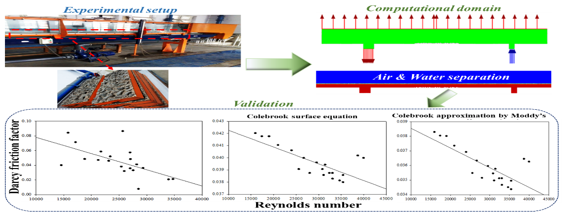
Turbulent flow over gravel beds in open channels is a fundamental yet complex problem in hydraulic engineering, as flow behavior is highly sensitive to channel geometry and bed roughness. In this study, the Volume of Fluid (VOF) method coupled with the standard k-ε turbulence model is employed to simulate air-water interactions over gravel beds, with open boundary conditions capturing realistic channel-atmosphere interactions. Numerical simulations are performed to examine how channel design influences the relationship between the friction factor (f) and the Reynolds number (RN). Velocity and VOF contours indicate peak flow near the inlet, with a maximum velocity of 0.64 m/s. The simulations show strong agreement with theoretical predictions, yielding a correlation coefficient of 0.99 for RN, while f and Chezy’s coefficient (C) reach 0.75 and 0.71, respectively. Comparison with experimental measurements shows deviations of approximately 17% for RN, 25% for f, and 12% for C. Moreover, further analysis confirms an inverse linear relationship between f and RN, in accordance with classical models such as Bazin’s curves, the Colebrook equation, and Moody’s approximation. Overall, the results demonstrate that the proposed numerical framework reliably captures flow dynamics over gravel beds, offering a robust tool for hydraulic design and performance assessment of open channels.Graphic Abstract
Keywords
In engineering applications, streams and rivers are considered the primary examples of open channel flows. Understanding how the general characteristics of open channels depend on cross-sectional geometry is essential, as it allows engineers to evaluate flow capacity across different shapes [1]. In mountainous regions, gravel transport is common, and numerous studies have investigated how gravel beds influence flow behavior [2].
Surface or bed roughness directly affects the Reynolds number (RN) by increasing its value. To account for roughness effects in flow channels, scalable wall functions must be applied to various mesh types to assess how roughness influences fluid dynamics and RN [3,4]. Free surface effects can be captured using the Volume of Fluid (VOF) model in computational fluid dynamics (CFD) simulations, with the key element in open channel models being the air-water interface. Evaluating RN is crucial for understanding flow performance in channels with rough beds [4,5]. Turbulence near the free surface is particularly important because vorticity, momentum, heat, and mass transfer are largely governed by surface dynamics. Free surface behavior presents significant challenges in rough bed flows, and knowledge of two-phase interactions remains limited [6].
Roughness is not confined to the bed; it also manifests at the free surface through surface tension between phases, and its magnitude depends on the roughness height [7]. Understanding flow development in rough channels with turbulent near-surface interactions is complex. To capture these effects, the free surface was modeled using the VOF approach coupled with the standard k-ε turbulence model. Roughness impacts velocity magnitude and alters the direction of flow vectors over rough surfaces [1]. Gravel roughness in rectangular channels significantly affects flow resistance and RN, as well as transitions between laminar, transitional, and turbulent regimes [8]. In open channels, the critical Reynolds number marks the transition from laminar to turbulent flow, and surface roughness increases RN while influencing turbulent characteristics [8].
Open channel flows are characterized by a free surface exposed to the atmosphere. Key parameters such as the friction coefficient and shear velocity are essential for quantifying flow resistance; however, accurately estimating these factors remains challenging. Traditional open channel equations often provide imprecise results due to difficulties in determining energy slopes and maintaining steady, uniform flow in human-made channels [9]. Channels can be natural or artificial, with bed roughness manipulated in the latter to control flow. The friction coefficient is a critical parameter for predicting flow velocity and ensuring accurate design. While CFD research often focuses on circular pipe flows, theoretical approaches remain important for open channel experiments due to computational complexity [10].
Recent advances in numerical modeling have demonstrated the utility of CFD in simulating complex open channel and rough bed flows, validated against laboratory data. For example, Yu et al. [11] conducted a comparative 2D CFD study of turbulent flow in open channels with emerged vegetation using multiple RANS turbulence closures, highlighting the influence of model choice on turbulence predictions and mean velocity structures while confirming the applicability of standard k-ε formulations. Xie et al. [12] employed OpenFOAM to simulate rough bed channels, showing strong agreement with experiments and capturing roughness effects on turbulent structures. Large-eddy simulation has been applied to free surface gravel bed flows to better resolve turbulence and bed interaction phenomena beyond RANS capabilities, providing insight into near-bed vortical behavior and free surface dynamics [13]. Additionally, direct numerical simulations of turbulent open channel flows at moderately high Reynolds numbers have documented detailed turbulence statistics and free surface effects, demonstrating the continuing development of high-fidelity computational approaches [14,15].
Determining roughness parameters remains challenging and often requires field measurements or laboratory experiments [3]. The friction factor is widely recognized as a critical variable for predicting flow behavior [16]. In laminar open channel flows, channel shape significantly affects the relationship between the friction factor and RN for non-Newtonian fluids [7]. Bed roughness enhances turbulence, typically reducing velocity near the rough surface while increasing it at the free surface [17]. Open channel studies are used to forecast flow patterns for a variety of scenarios, including stormwater, drainage, sediment transport, and suspended particle tracking in turbulent flows [2,18]. The impact of roughness on flow characteristics varies with channel design and configuration [2].
In this study, experimental investigations were conducted to assess flow resistance in a rectangular open channel with uniformly distributed gravel. Complementary numerical simulations were performed in ANSYS using VOF coupled with the k-ε turbulence model. The objectives were to evaluate the effect of designed roughness on flow, quantify the friction factor-RN relationship, and compare experimental and numerical results for validation. The observed f-RN relationship aligns with previous studies, providing insights into the hydraulic performance of gravel-lined channels. These findings have practical implications for improved flow prediction, optimized channel design, flood risk assessment, sediment transport management, and environmental considerations in hydraulic engineering [1,12,13].
2.1 Experimental and Numerical Setup
A rectangular flume with a gravel bed was used for the experiments. The flume measured 10 m in length and 0.3 m in width. All experiments were conducted in the Hydraulics Engineering Laboratory of the Department of Civil Engineering, University of Engineering and Technology (UET), Lahore. The channel was glass-sided with a depth of 0.75 m and featured an adjustable tailgate at the downstream end to regulate flow depth.
Discharge was supplied to the channel via a centrifugal pump, passing through a honeycomb flow straightener to ensure uniform and smooth distribution across the channel width. At the downstream end, water entered a sediment tank where sediments were trapped, and the flow then discharged from the main channel. A plan view of the laboratory flume and experimental setup is shown in Fig. 1.
Flow depth measurements were obtained using a hook gauge mounted on top of the flume, allowing precise determination of water surface elevation at multiple locations along the channel. These measurements were used to compute hydraulic parameters such as flow area (A) and hydraulic radius (Rh). Flow velocity (V) was calculated indirectly from the measured discharge (Q) and corresponding flow area, following standard open-channel flow procedures.
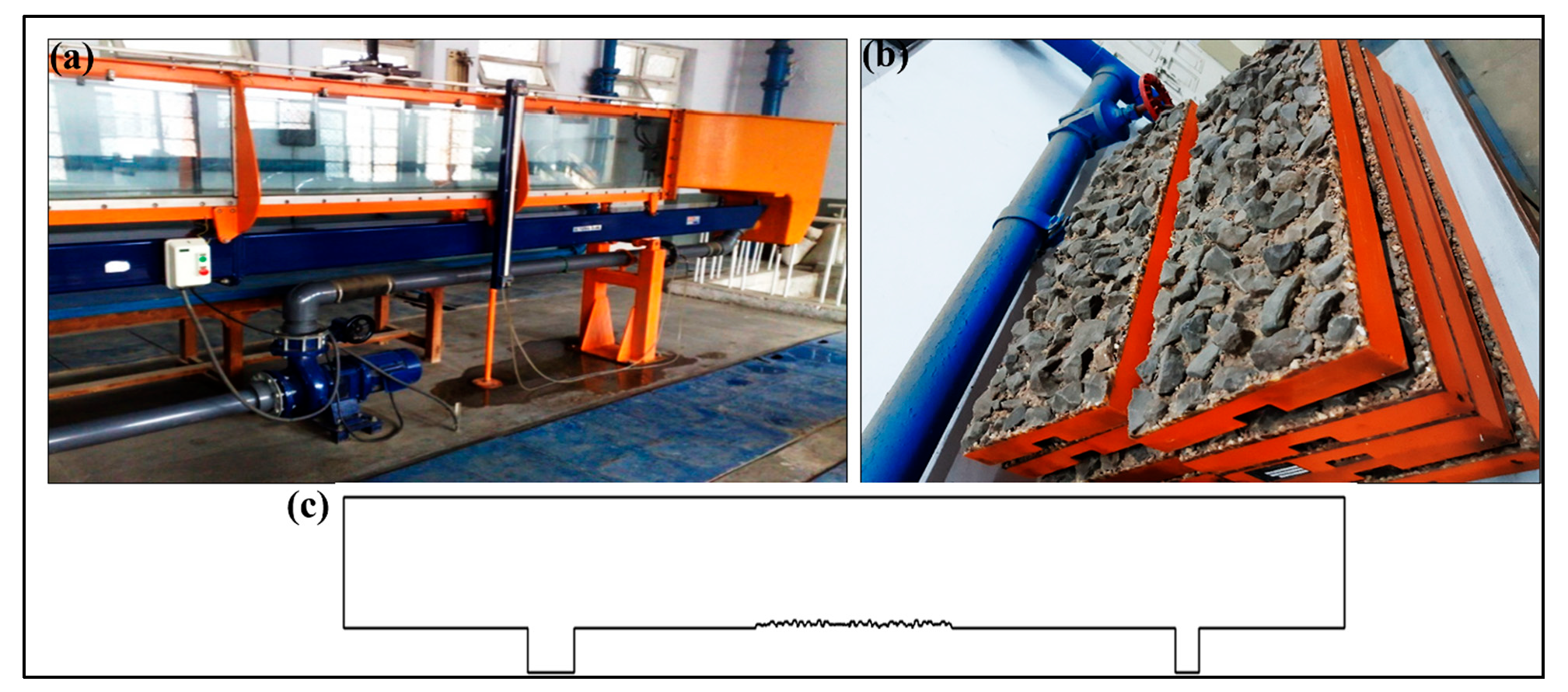
Figure 1: Experimental setup: (a) rectangular flume used for open channel experiments, (b) gravel bed segments (1 m each) installed in the flume, (c) 2D numerical model of the channel with the gravel bed surface.
Since the flow was non-uniform along the channel, the bed slope (So) could not be reliably used to estimate Manning’s “n”. The gravel bed (Fig. 1b) was prepared on a horizontal wooden plank measuring 1 m × 0.3 m, following Bazin’s channel bed characteristics [1]. The gravel layer was then installed in the flume to reproduce realistic roughness conditions. A corresponding 2D numerical model (Fig. 1c) was generated in AutoCAD to incorporate gravel bed effects for open channel flow simulations using ANSYS Fluent.
In the VOF approach, a volume fraction α describes the local presence of one phase (e.g., liquid) in a multiphase system. The governing equations (Eqs. (1)–(5)) consist of the conservation of volume fraction, the incompressible continuity equation, and the momentum equation (Navier-Stokes with surface force).
In numerical simulations, meshing plays a critical role in accurately predicting fluid behavior. A refined mesh was applied in regions of interest, particularly near the gravel bed and the free surface. Triangular elements with a characteristic length of 0.001 m were employed, resulting in 39,717 cells, 60,225 faces, and 20,509 nodes, following the grid refinement study shown in Fig. 2. The mesh quality was evaluated using skewness and orthogonality criteria to ensure numerical stability and solution reliability. No highly skewed or poorly orthogonal elements were detected. Additional refinement near the gravel bed and free-surface regions enabled accurate resolution of velocity gradients and turbulence effects. Smooth convergence behavior and stable residual reduction confirmed the adequacy of the adopted mesh for the present simulations.
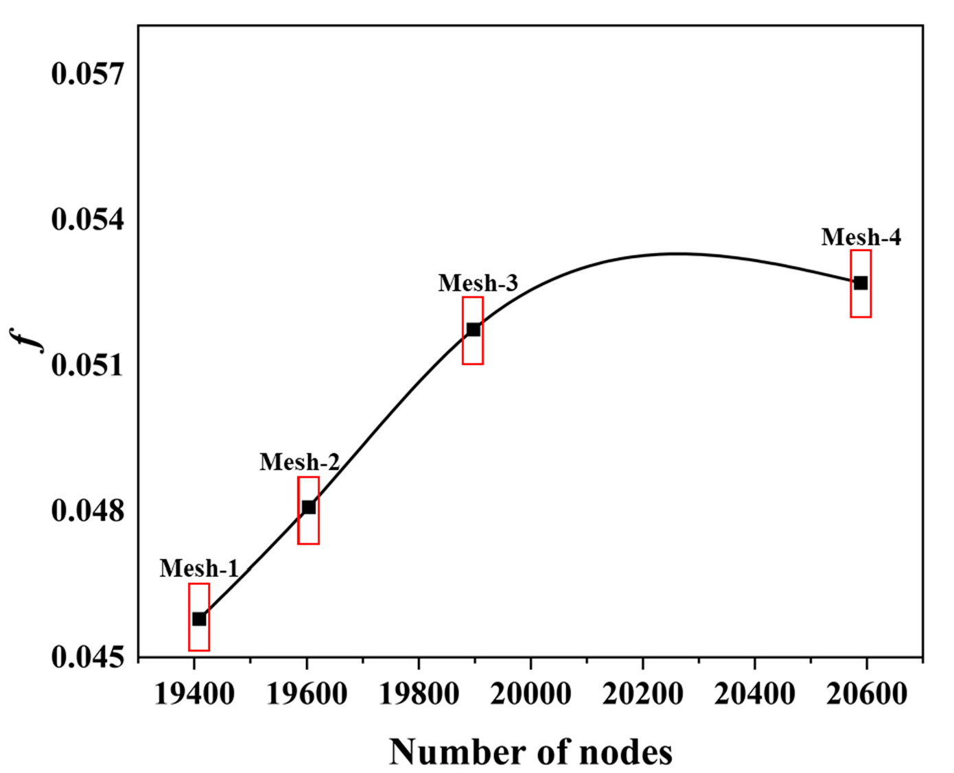
Figure 2: Grid refinement against friction factor (f).
The multiphase simulations involved air and water, with gravitational acceleration of 9.81 m/s2 applied in the vertical direction and a free surface condition specified. Numerical simulations were performed in ANSYS Fluent (version 2020). A steady-state formulation was adopted to investigate mean flow behavior and resistance characteristics under fully developed turbulent flow conditions. The VOF model captured air-water interactions, and turbulence was modeled using the standard k-ε model. Pressure-velocity coupling was handled using the SIMPLE algorithm, and second-order upwind schemes were applied to momentum and turbulence equations for improved accuracy. Convergence was ensured by reducing residuals below 10−5 for continuity and momentum and below 10−6 for turbulence quantities, while monitoring the stabilization of key hydraulic parameters such as velocity and discharge.
The experimental and numerical workflow employed in this study is summarized in the flow chart shown in Fig. 3.
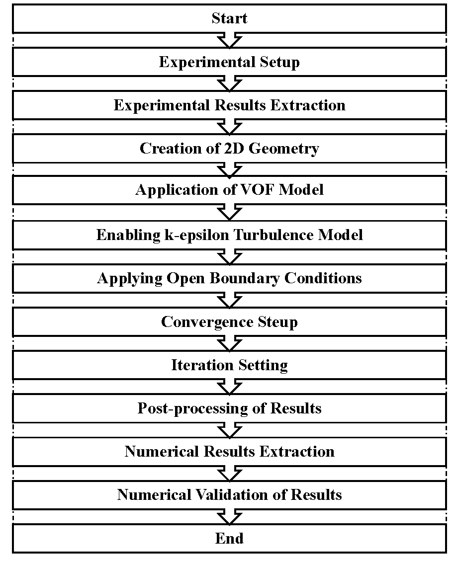
Figure 3: Flow chart illustrating the methodology of the experimental and numerical investigation.
While applying a free surface boundary condition, the implicit method was used, and a no-slip condition was enforced at all channel walls [5,14]. Under the no-slip condition, the wall is assumed stationary, and the fluid velocity at the wall is zero [19]. The hydraulic grade line (HGL) provides information on pressure at various sections, which is essential for the structural design of channels. For steady flow, the flow depth at a given cross-section remains constant (Eq. (6)). Prismatic and man-made channels typically exhibit average steady flow conditions [1,20].
In uniform flow, the flow depth, velocity, acceleration, slope, and channel cross-section remain constant along the distance between two sections of the channel (Eq. (7)) [15].
In steady-uniform flow, characteristics such as discharge, velocity, and flow area remain constant over both time and distance. In contrast, steady-non-uniform flow describes a regime where these properties remain consistent over time but vary along the channel length [19]. Unsteady-uniform flow is characterized by fluid properties that remain consistent along a specific distance but vary over time. Conversely, unsteady-non-uniform flow refers to a regime in which fluid properties vary with both time and distance [1].
Although the flow regime depends on the roughness configuration of the channel, hydraulic dynamics are also governed by fluid properties. Flow is categorized as laminar or turbulent based on the relative influence of viscous and inertial forces [20]. According to RN, flow is considered laminar when RN < 500. For pipe flow, the laminar-to-turbulent transition occurs approximately between RN = 2000 and 50,000, while in open channels, the transition range extends from RN = 500 to 12,500 [21]. The relationship between viscous and inertial forces can be expressed in terms of RN (Eq. (8)).
According to Manning’s formulation, the horizontal component of gravitational force is balanced by the shear resistance of the bed [22,24]. The Manning equation provides an empirical relationship between flow area, channel slope, and flow velocity, with Manning’s coefficient representing the friction exerted by channel bed roughness (Eq. (11)). As channel roughness increases, Manning’s n correspondingly increases [1,15,18].
2.2 Validation of Numerical Results
The Colebrook equation provides a computational method for determining f in fully developed pipe flows or ducts, and it can also be applied to approximate open channel flow. This equation is primarily used for turbulent flows, including high-intensity fluid regimes approaching their upper limits. The mathematical formulation for f is given in Eq. (14) [14,25].
The second method used for numerical validation is the Haaland approximation [16,26]. This method is also applicable to turbulent flow conditions, although turbulent flows are restricted to a specific RN range. The RN for which this approximation is valid extends from a minimum of 4000 to a maximum of 5 × 10⁸. The corresponding mathematical expression is given in Eq. (15). In addition to empirical and semi-empirical equations, data-driven approaches such as artificial neural networks have also been applied to predict friction factor behavior in open channel flow with satisfactory accuracy [27,28].
Several statistical tests were performed to evaluate the performance of the experimental and numerical results, as summarized in Table 1. Here, Ni represents the numerical values, while O denotes the observed data. The symbol
Table 1: Description of statistical metrics.
| Statistical Indicators | Formulas | Unit | Best Values |
|---|---|---|---|
| Correlation Coefficient (r) | | - | 1 |
| Percentage Error (PE) | | % | 0 |
| Mean Absolute Error (MAE) | | - | 0 |
| Root Mean Square Error (RMSE) | | - | 0 |
The observed inverse relationship between f and RN (Fig. 4) reflects the progressive dominance of inertial forces over viscous effects as flow intensity increases. At lower RN, flow resistance is strongly influenced by bed roughness and near-bed turbulence, resulting in higher f. As RN increases, the relative effect of roughness diminishes, and the flow becomes fully turbulent, reducing frictional resistance. This behavior is consistent with classical hydraulic theory and well-established empirical formulations, including Bazin’s curves and the Colebrook and Moody relationships [1,14]. Comparable inverse trends between f and RN have also been reported for vegetated and rough open channel flows under turbulent conditions [26,29].
Similarly, the positive relationship between C and V (Fig. 5) indicates an increase in flow conveyance efficiency with higher velocity, as increased momentum allows the flow to overcome bed-induced resistance more effectively. The agreement between experimental observations and numerical predictions demonstrates that the adopted modeling approach can capture the dominant hydraulic mechanisms governing gravel-bed open channel flow, despite the inherent simplifications of depth-averaged and two-dimensional simulations.
As discharge (Q) increases, the flow area (A) also increases, which interacts with more roughness, ultimately raising Manning’s n (Table 2). The relationship between V and n for a gravel bed was found to be exponential and inverse (Table 2 and Table 3), with higher velocities corresponding to lower n values. This occurs because increased velocity reduces flow depth, causing the flow to approach supercritical conditions, as evident from the specific energy diagrams [10].
During experiments with the gravel bed, several interesting behaviors were observed. The relationship between f and RN was linear and inverse (Fig. 4), showing strong correlation with Bazin’s curve [1]. Notably, the C value corresponding to the 18th experimental observation (Table 2) was unusually high compared to the rest of the dataset. This outlier is attributed to measurement uncertainty in flow depth at different channel locations during that run. The resulting very small energy slope produced an unrealistically high C value, which does not represent the actual hydraulic behavior of the gravel-bed channel. This data point is retained for completeness and transparency, but it is not considered representative of the overall flow trend.
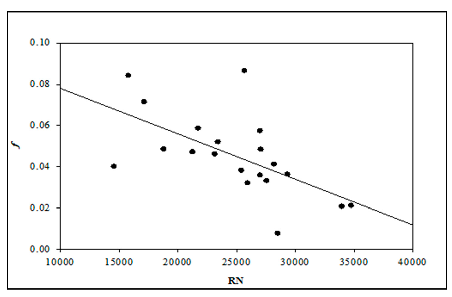
Figure 4: Relationship between the f and RN from experimental measurements in a gravel-bed open channel.
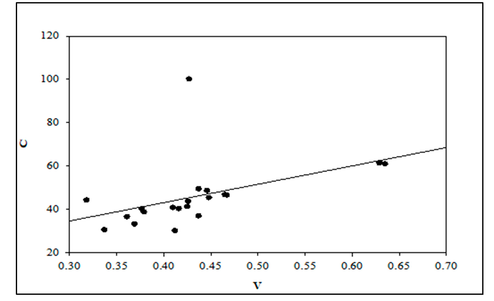
Figure 5: Relationship between C and V from experimental measurements in a gravel-bed open channel.
Table 2: Experimental observations and calculated values for the estimation of flow parameters in a gravel-bed open channel.
| Kinematics Viscosity = 1.00325 × 10⁻⁶ m2/s | Experimental Observations | Z1 = So × L = 0.005 × 2.5 = 0.0125 m | |||||||||||||
|---|---|---|---|---|---|---|---|---|---|---|---|---|---|---|---|
| B = 0.3 m | Z2 = So × L = 0.005 × 5 = 0.025 = m | ||||||||||||||
| Sr. No. | Q | Depth of Flow | E1 | E2 | hL | SE (hL/L) | Rh | V | C | n | f | RN | |||
| Y1 | Y2 | Y3 | Yavg. | ||||||||||||
| m3/s | mm | m | m | m | m | - | m | m/s | |||||||
| 1 | 0.0063 | 73.0 | 65.0 | 61.0 | 0.066 | 0.090 | 0.095 | 0.006 | 0.001 | 0.046 | 0.318 | 44.23 | 0.0135 | 0.0401 | 14,566.68 |
| 2 | 0.0075 | 67.0 | 68.0 | 67.8 | 0.068 | 0.087 | 0.100 | 0.013 | 0.003 | 0.047 | 0.369 | 33.14 | 0.0181 | 0.0715 | 17,134.11 |
| 3 | 0.0069 | 69.1 | 69.6 | 67.1 | 0.069 | 0.087 | 0.100 | 0.013 | 0.003 | 0.047 | 0.337 | 30.52 | 0.0197 | 0.0843 | 15,790.40 |
| 4 | 0.0085 | 78.6 | 74.1 | 72.1 | 0.075 | 0.098 | 0.107 | 0.009 | 0.002 | 0.050 | 0.377 | 40.18 | 0.0151 | 0.0486 | 18,795.61 |
| 5 | 0.0098 | 83.2 | 79.7 | 76.1 | 0.080 | 0.104 | 0.113 | 0.010 | 0.002 | 0.052 | 0.410 | 40.78 | 0.0150 | 0.0472 | 21,255.30 |
| 6 | 0.0110 | 88.2 | 84.7 | 84.6 | 0.086 | 0.109 | 0.119 | 0.010 | 0.002 | 0.055 | 0.425 | 41.25 | 0.0149 | 0.0461 | 23,144.57 |
| 7 | 0.0123 | 95.8 | 90.8 | 88.7 | 0.092 | 0.118 | 0.126 | 0.009 | 0.002 | 0.057 | 0.448 | 45.35 | 0.0137 | 0.0382 | 25,408.94 |
| 8 | 0.0133 | 99.6 | 94.5 | 91.4 | 0.095 | 0.122 | 0.131 | 0.009 | 0.002 | 0.058 | 0.465 | 46.73 | 0.0133 | 0.0359 | 27,008.08 |
| 9 | 0.0130 | 104.8 | 97.5 | 94.5 | 0.099 | 0.126 | 0.133 | 0.007 | 0.001 | 0.060 | 0.437 | 49.42 | 0.0126 | 0.0321 | 25,942.73 |
| 10 | 0.0141 | 111.1 | 104.1 | 102.1 | 0.106 | 0.133 | 0.140 | 0.007 | 0.001 | 0.062 | 0.446 | 48.61 | 0.0129 | 0.0332 | 27,550.89 |
| 11 | 0.0152 | 113.1 | 107.5 | 105.5 | 0.109 | 0.136 | 0.144 | 0.008 | 0.002 | 0.063 | 0.467 | 46.51 | 0.0136 | 0.0363 | 29,336.43 |
| 12 | 0.0110 | 105.0 | 99.9 | 98.8 | 0.101 | 0.124 | 0.132 | 0.008 | 0.002 | 0.060 | 0.361 | 36.57 | 0.0171 | 0.0587 | 21,725.86 |
| 13 | 0.0120 | 110.0 | 104.5 | 101.6 | 0.105 | 0.129 | 0.137 | 0.008 | 0.002 | 0.062 | 0.379 | 38.79 | 0.0162 | 0.0521 | 23,405.85 |
| 14 | 0.0133 | 105.7 | 108.6 | 108.0 | 0.107 | 0.127 | 0.142 | 0.015 | 0.003 | 0.063 | 0.412 | 30.10 | 0.0209 | 0.0866 | 25,676.62 |
| 15 | 0.0139 | 106.0 | 104.5 | 106.6 | 0.106 | 0.128 | 0.139 | 0.011 | 0.002 | 0.062 | 0.437 | 36.94 | 0.0170 | 0.0575 | 27,000.63 |
| 16 | 0.0144 | 118.3 | 113.2 | 115.0 | 0.116 | 0.139 | 0.147 | 0.008 | 0.002 | 0.065 | 0.416 | 40.29 | 0.0157 | 0.0484 | 27,066.46 |
| 17 | 0.0152 | 122.7 | 116.4 | 118.6 | 0.119 | 0.144 | 0.151 | 0.007 | 0.001 | 0.066 | 0.426 | 43.62 | 0.0146 | 0.0412 | 28,188.69 |
| 18 | 0.0155 | 125.6 | 112.3 | 124.5 | 0.121 | 0.147 | 0.148 | 0.001 | 0.001 | 0.067 | 0.427 | 100.16 | 0.0064 | 0.0078 | 28,504.11 |
| 19 | 0.0160 | 90.0 | 85.0 | 79.5 | 0.085 | 0.120 | 0.130 | 0.010 | 0.002 | 0.054 | 0.629 | 61.41 | 0.0100 | 0.0208 | 33,947.87 |
| 20 | 0.0165 | 92.0 | 87.5 | 80.0 | 0.087 | 0.123 | 0.133 | 0.010 | 0.002 | 0.055 | 0.635 | 60.90 | 0.0101 | 0.0212 | 34,745.43 |
Table 3: Numerical observations and computed hydraulic parameters for the gravel-bed open channel.
| Kinematics Viscosity = 1.00325 × 10⁻⁶ m2/s | Numerical Observations | Dynamic Viscosity = 0.001003 kg·m/s | |||||||||||||
|---|---|---|---|---|---|---|---|---|---|---|---|---|---|---|---|
| B = 0.3 m | |||||||||||||||
| Sr. No. | Q | Depth of Flow | E1 | E2 | hL | SE (hL/L) | Rh | P | V | C | f | RN | |||
| Y1 | Y2 | Y3 | Yavg. | ||||||||||||
| m3/s | mm | m | m | m | m | - | m | m | m/s | ||||||
| 1 | 0.0063 | 73 | 65 | 61 | 0.066 | 0.09 | 0.095 | 0.006 | 0.001 | 0.046 | 0.43267 | 0.318 | 41.60 | 0.04535 | 15,962.00 |
| 2 | 0.0075 | 67 | 68 | 67.8 | 0.068 | 0.087 | 0.1 | 0.013 | 0.003 | 0.047 | 0.4352 | 0.369 | 38.59 | 0.05270 | 19,008.30 |
| 3 | 0.0069 | 69.1 | 69.6 | 67.1 | 0.069 | 0.087 | 0.1 | 0.013 | 0.003 | 0.047 | 0.4372 | 0.337 | 40.40 | 0.04809 | 17,397.30 |
| 4 | 0.0085 | 78.6 | 74.1 | 72.1 | 0.075 | 0.098 | 0.107 | 0.009 | 0.002 | 0.05 | 0.44987 | 0.377 | 38.17 | 0.05386 | 20,984.80 |
| 5 | 0.0098 | 83.2 | 79.7 | 76.1 | 0.08 | 0.104 | 0.113 | 0.01 | 0.002 | 0.052 | 0.45933 | 0.41 | 40.88 | 0.04696 | 24,005.60 |
| 6 | 0.011 | 88.2 | 84.7 | 84.6 | 0.086 | 0.109 | 0.119 | 0.01 | 0.002 | 0.055 | 0.47167 | 0.425 | 41.08 | 0.04650 | 26,686.50 |
| 7 | 0.0123 | 95.8 | 90.8 | 88.7 | 0.092 | 0.118 | 0.126 | 0.009 | 0.002 | 0.057 | 0.48353 | 0.448 | 50.02 | 0.03137 | 29,554.30 |
| 8 | 0.0133 | 99.6 | 94.5 | 91.4 | 0.095 | 0.122 | 0.131 | 0.009 | 0.002 | 0.058 | 0.49033 | 0.465 | 50.08 | 0.03130 | 31,432.90 |
| 9 | 0.013 | 104.8 | 97.5 | 94.5 | 0.099 | 0.126 | 0.133 | 0.007 | 0.001 | 0.06 | 0.49787 | 0.437 | 50.69 | 0.03054 | 30,849.30 |
| 10 | 0.0141 | 111.1 | 104.1 | 102.1 | 0.106 | 0.133 | 0.14 | 0.007 | 0.001 | 0.062 | 0.51153 | 0.446 | 49.46 | 0.03209 | 33,065.00 |
| 11 | 0.0152 | 113.1 | 107.5 | 105.5 | 0.109 | 0.136 | 0.144 | 0.008 | 0.002 | 0.063 | 0.5174 | 0.467 | 50.95 | 0.03023 | 35,426.80 |
| 12 | 0.011 | 105 | 99.9 | 98.8 | 0.101 | 0.124 | 0.132 | 0.008 | 0.002 | 0.06 | 0.50247 | 0.361 | 35.42 | 0.06254 | 25,599.10 |
| 13 | 0.012 | 110 | 104.5 | 101.6 | 0.105 | 0.129 | 0.137 | 0.008 | 0.002 | 0.062 | 0.51073 | 0.379 | 36.50 | 0.05892 | 28,030.10 |
| 14 | 0.0133 | 105.7 | 108.6 | 108 | 0.107 | 0.127 | 0.142 | 0.015 | 0.003 | 0.063 | 0.51487 | 0.412 | 38.07 | 0.05414 | 31,108.60 |
| 15 | 0.0139 | 106 | 104.5 | 106.6 | 0.106 | 0.128 | 0.139 | 0.011 | 0.002 | 0.062 | 0.5114 | 0.437 | 39.02 | 0.05155 | 32,397.50 |
| 16 | 0.0144 | 118.3 | 113.2 | 115 | 0.116 | 0.139 | 0.147 | 0.008 | 0.002 | 0.065 | 0.531 | 0.416 | 53.42 | 0.02750 | 33,092.60 |
| 17 | 0.0152 | 122.7 | 116.4 | 118.6 | 0.119 | 0.144 | 0.151 | 0.007 | 0.001 | 0.066 | 0.53847 | 0.426 | 55.74 | 0.02526 | 34,648.00 |
| 18 | 0.0155 | 125.6 | 112.3 | 124.5 | 0.121 | 0.147 | 0.148 | 0.001 | 0.001 | 0.067 | 0.5416 | 0.427 | 59.01 | 0.02254 | 35,418.70 |
| 19 | 0.016 | 90 | 85 | 79.5 | 0.085 | 0.12 | 0.13 | 0.01 | 0.002 | 0.054 | 0.46967 | 0.629 | 56.37 | 0.02470 | 38,695.70 |
| 20 | 0.0165 | 92 | 87.5 | 80 | 0.087 | 0.123 | 0.133 | 0.01 | 0.002 | 0.055 | 0.473 | 0.635 | 60.77 | 0.02125 | 39,976.00 |
Fig. 4 illustrates a negative correlation between f and RN. As RN increases, indicating a transition from laminar to turbulent flow, f decreases. This behavior is typical in fluid dynamics, as turbulent flow, associated with higher RN, generally produces lower frictional losses. The fitted trend line highlights this inverse relationship, emphasizing how increased turbulence reduces f.
The C value for the 18th gravel-bed measurement was unusually high, recorded as 100. This anomaly is attributed to measurement errors in flow depth at multiple channel locations. Specifically, the energy line slope for this reading was extremely low, suggesting negligible head loss, which is physically unrealistic for a gravel-bed channel.
Similarly, Fig. 5 shows a positive correlation between C and V. As V increases, C also increases, as indicated by the upward trend of the fitted line. This relationship appears to be linear, with the majority of data points following a consistent increasing trend, suggesting that higher flow velocities correspond to higher Chezy coefficients.
The numerical results were evaluated using ANSYS Fluent. In the simulations, the free surface was defined by specifying the fluid depth in the modeled open-flow channel. Air was assigned as phase-1, and water as phase-2, allowing computation of f, C, and RN. The effects of gravel-bed roughness were analyzed within the phase-2 region, while phase-1 served as the boundary layer for the free surface.
For comparison with experimental data, V was plotted against C, as shown in Fig. 6. The numerical results indicate greater stability in C values relative to the experimental measurements. Fig. 6 demonstrates a positive linear relationship between C and V, with both variables increasing consistently. As V increases, C also tends to rise, as indicated by the upward-sloping trend line. However, the data points exhibit some variability, particularly at higher V values, suggesting that while a general increasing trend exists, deviations occur. Overall, the plot indicates that C is directly influenced by V, though with a certain degree of fluctuation.
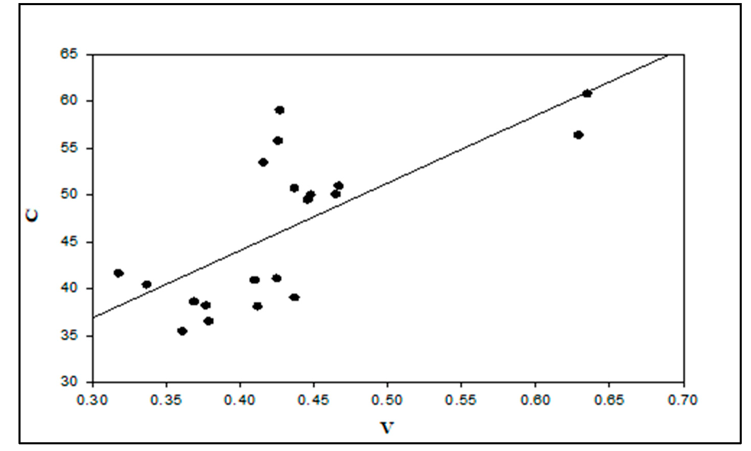
Figure 6: Relationship between C and V obtained from numerical simulations for a gravel-bed open channel.
Fig. 7 illustrates a negative relationship between f and RN. As RN increases, f decreases, as shown by the downward-sloping trend line. This behavior aligns with fluid dynamics principles, where higher RN, typically associated with more turbulent flow, corresponds to lower frictional losses. The plot confirms a clear inverse correlation, indicating that as flow becomes more turbulent, the friction factor diminishes.
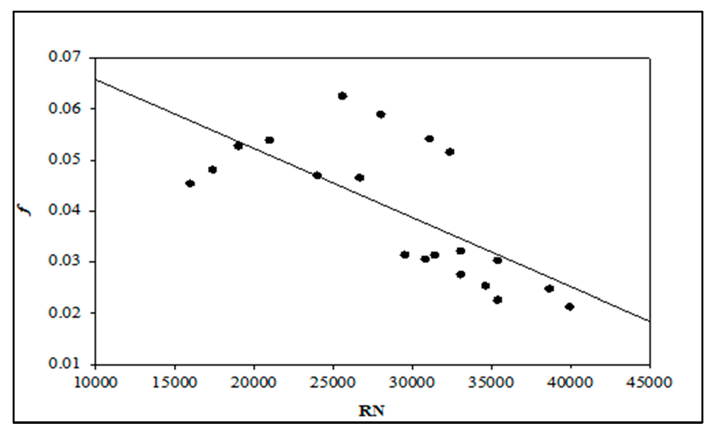
Figure 7: Relationship between the f and RN obtained from numerical simulations for a gravel-bed open channel.
Table 4 presents statistical indicators for three variables: f, RN, and C. The correlation coefficient (r) indicates that RN exhibits the strongest positive correlation, followed by f and C. The percentage error (PE) shows that RN has the lowest error, whereas C and f display higher errors. In terms of mean absolute error (MAE), RN has the highest value, reflecting larger prediction deviations compared to f and C. Similarly, the root mean square error (RMSE) is greatest for RN, suggesting that RN experiences the largest prediction discrepancies, followed by C and f. Overall, RN demonstrates strong correlations but also exhibits substantial prediction errors.
Table 4: Result of statistical test for experimental and numerical hydraulic parameters.
| Statistical Indicators | f | RN | C |
|---|---|---|---|
| R | 0.753 | 0.991 | 0.715 |
| PE | 25.4% | 17.01% | 12.14% |
| MAE | 0.009 | 4357.19 | 5.994 |
| RMSE | 0.014 | 4647.83 | 10.737 |
Computational studies inherently involve some degree of error, as numerical models attempt to replicate real-world physical systems but cannot achieve exact correspondence with experimental conditions. The differences between the experimental and numerical results are illustrated in Fig. 8a,b.
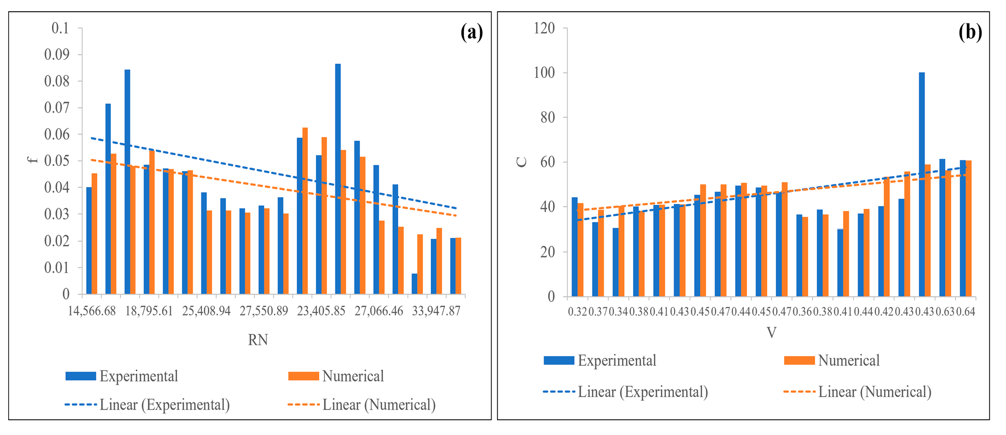
Figure 8: Comparison between experimental and numerical results; (a) f versus RN; (b) C versus V.
The observed discrepancies arise from modeling errors, which occur when converting a real physical system into a numerical model. These errors represent deviations between experimental and numerical results. In practice, it is not possible to replicate the exact geometry of the gravel bed within the modeling software; instead, the numerical model approximates the bed based on available simulation data.
The results generally follow the expected trends: lower f values correspond to higher RN, consistent with Bazin’s curve, which shows that as RN increases, friction decreases. Similarly, the relationship between C and V remains direct, while the f versus RN relationship is inverse. However, due to the inherent complexity of the flow and the approximations in the numerical model, the results cannot perfectly match the exact physical behavior.
Validation of Experimental and Numerical Results
Effective presentation of results is crucial for conveying the findings clearly and ensuring a proper understanding of the investigated problem. In the numerical simulations, contour plots are used to visualize the flow patterns and solution distribution. These plots serve as a conceptual framework for the model, guiding the interpretation of results during the post-processing stage and facilitating accurate analysis of flow behavior.
The velocity magnitude contours indicate that the fluid follows the prescribed flow direction and boundary conditions, as illustrated in Fig. 9. Accurate interpretation of the VOF model requires careful examination of these contours to ensure consistency with the defined computational domain. In the VOF contours, the red regions represent the water phase, while the blue regions correspond to the air phase, as shown in Fig. 10.
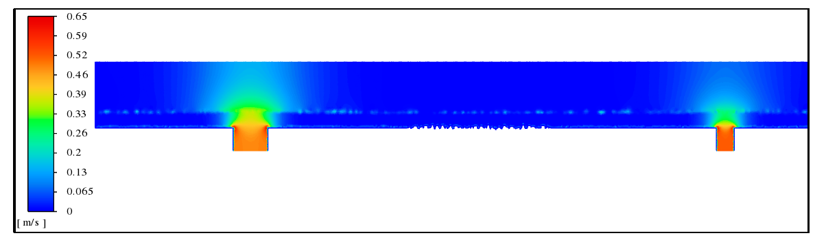
Figure 9: Velocity magnitude contour obtained from numerical simulations.
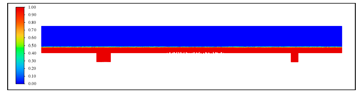
Figure 10: VOF contour for the water phase obtained from numerical simulations.
In the open channel flume, the low-density fluid is air, designated as phase-1 in the simulations to represent the upper region of the flume. In the VOF contours, red indicates the air phase, while blue represents the water phase. The VOF distribution for air is shown in Fig. 11.
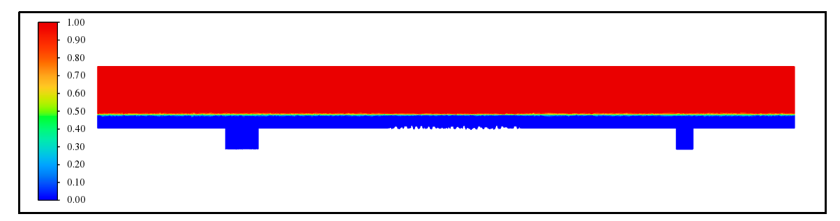
Figure 11: VOF air contour for the air phase obtained from numerical simulations.
Investigating flow in an open channel is a challenging task, particularly for non-prismatic channels. To assess the accuracy of the numerical results, validation was performed using two approximation techniques: the Colebrook free-surface equation and the Colebrook-Moody approximation (Fig. 12). Both methods confirmed the f-RN relationship, demonstrating the expected decrease in f as RN increases.
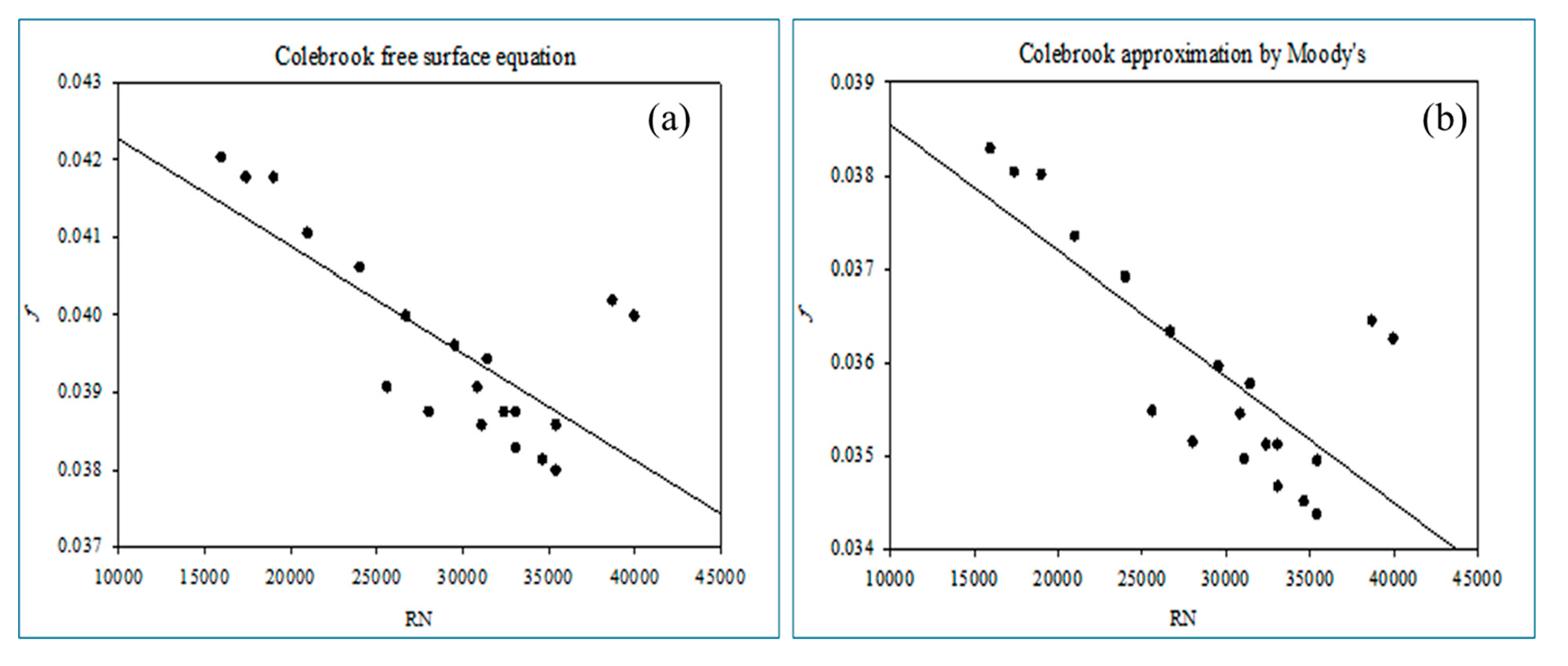
Figure 12: Relationship between f and RN for the gravel-bed open channel using: (a) Colebrook free-surface equation, (b) Colebrook approximation by Moody’s method.
This study combined laboratory experiments with numerical modeling to better understand flow resistance in a gravel-bed open channel and to examine how classical hydraulic relationships perform when applied using modern CFD tools.
- 1.The main objective was to investigate the relationship between the friction factor and Reynolds number in a gravel-bed open channel and to assess how bed roughness influences flow resistance under turbulent conditions.
- 2.Experimental tests were carried out in a rectangular flume with a uniformly distributed gravel bed, where flow depths were measured using a hook gauge and hydraulic parameters were obtained from measured discharge and channel geometry.
- 3.A two-dimensional CFD model was developed using the Volume of Fluid (VOF) approach coupled with the standard k-ε turbulence model to represent free-surface flow and turbulence effects.
- 4.The results consistently showed that the friction factor decreases as the Reynolds number increases, indicating that at higher flow intensities the influence of bed roughness becomes less dominant.
- 5.A clear increasing trend was also observed between flow velocity and Chezy’s coefficient, suggesting improved flow conveyance with increasing velocity.
- 6.The numerical predictions showed good agreement with the experimental data, with a strong correlation for the Reynolds number (r ≈ 0.99) and reasonable correlations for the friction factor (r ≈ 0.75) and Chezy’s coefficient (r ≈ 0.71).
- 7.The average percentage differences between numerical and experimental results were about 17% for Reynolds number, 25% for the friction factor, and 12% for Chezy’s coefficient, which are acceptable considering experimental uncertainty and modeling simplifications.
- 8.Validation using the Colebrook equation and Moody’s approximation further supported the observed inverse relationship between friction factor and Reynolds number.
- 9.The overall findings indicate that the combined experimental-numerical approach used in this study is suitable for analyzing gravel-bed open channel flows and can support practical hydraulic assessments and preliminary channel design.
- 10.Future work could extend this research by applying three-dimensional simulations, testing different gravel sizes and arrangements, and incorporating more advanced turbulence models to better resolve local flow structures.
In summary, the study confirms that classical resistance relationships such as those proposed by Bazin, Colebrook, and Moody remain applicable when supported by CFD modeling, providing a reliable framework for studying gravel-bed open channel flows.
Acknowledgement:
Funding Statement: The authors received no specific funding for this study.
Author Contributions: The authors confirm contribution to the paper as follows: Abdullah Abdullah: Experimental work, validation, and write-up. Ghulam Mohi Ud Din: CFD modelling, writing and review. Muhammad Aleem: Writing and review, formal analysis. Tipu Sultan: Supervision, writing, reviewing and editing. Muhammad Shareef Shazil: Methodology, writing, and statistical analysis. All authors reviewed and approved the final version of the manuscript.
Availability of Data and Materials: The data that support the findings of this study are available from the corresponding author upon reasonable request.
Ethics Approval: Not applicable.
Conflicts of Interest: The authors declare no conflict of interest.
References
1. Abbaspour A , Kia SH . Numerical investigation of turbulent open channel flow with semi-cylindrical rough beds. KSCE J Civ Eng. 2014; 18( 7): 2252– 60. doi:10.1007/s12205-014-0301-0. [Google Scholar] [CrossRef]
2. Abushandi E . Experimental investigations of open-channel flow and velocity to develop a predictive tool from a laboratory small scale to real-world large scale. Water Sci Technol. 2022; 86( 7): 1681– 92. doi:10.2166/wst.2022.287. [Google Scholar] [CrossRef]
3. Ahmad NA , Saiful Bahry SI , Md Ali Z , Mat Daud AM , Musa S . Effect of flow resistance in open rectangular channel. MATEC Web Conf. 2017; 97: 01107. doi:10.1051/matecconf/20179701107. [Google Scholar] [CrossRef]
4. Akan AO , Iyer SS . Open channel hydraulics. Oxford, UK: Butterworth-Heinemann; 2021. doi:10.1016/B978-0-12-821770-2.00001-4. [Google Scholar] [CrossRef]
5. Arthur JK . PIV measurements of open-channel turbulent flow under unconstrained conditions. Fluids. 2023; 8( 4): 135. doi:10.3390/fluids8040135. [Google Scholar] [CrossRef]
6. Buffington JM , Montgomery DR . Effects of hydraulic roughness on surface textures of gravel-bed rivers. Water Resour Res. 1999; 35( 11): 3507– 21. doi:10.1029/1999WR900138. [Google Scholar] [CrossRef]
7. Burger J , Haldenwang R , Alderman N . Friction factor-Reynolds number relationship for laminar flow of non-Newtonian fluids in open channels of different cross-sectional shapes. Chem Eng Sci. 2010; 65( 11): 3549– 56. doi:10.1016/j.ces.2010.02.040. [Google Scholar] [CrossRef]
8. Chanson H . Applications of the Bernoulli equation to open channel flows. In: Hydraulics of open channel flow. Amsterdam, The Netherlands: Elsevier; 2004. p. 21– 49. doi:10.1016/B978-075065978-9/50008-8. [Google Scholar] [CrossRef]
9. Cho YH , Dao MH , Nichols A . Computational fluid dynamics simulation of rough bed open channels using openFOAM. Front Environ Sci. 2022; 10: 981680. doi:10.3389/fenvs.2022.981680. [Google Scholar] [CrossRef]
10. Choo YM , Kim JG , Park SH . A study on the friction factor and Reynolds number relationship for flow in smooth and rough channels. Water. 2021; 13( 12): 1714. doi:10.3390/w13121714. [Google Scholar] [CrossRef]
11. Yu S , Dai H , Zhai Y , Liu M , Huai W . A comparative study on 2D CFD simulation of flow structure in an open channel with an emerged vegetation patch based on different RANS turbulence models. Water. 2022; 14( 18): 2873. doi:10.3390/w14182873. [Google Scholar] [CrossRef]
12. Xie Z , Lin B , Falconer RA , Nichols A , Tait SJ , Horoshenkov KV . Large-eddy simulation of turbulent free surface flow over a gravel bed. J Hydraul Res. 2022; 60( 2): 205– 19. doi:10.1080/00221686.2021.1908437. [Google Scholar] [CrossRef]
13. Yao J , Chen X , Hussain F . Direct numerical simulation of turbulent open channel flows at moderately high Reynolds numbers. J Fluid Mech. 2022; 953: A19. doi:10.1017/jfm.2022.942. [Google Scholar] [CrossRef]
14. Faruque A . Roughness effects on turbulence characteristics in an open channel flow. In: Boundary layer flows—Theory, applications and numerical methods. London, UK: IntechOpen; 2020. doi:10.5772/intechopen.85990. [Google Scholar] [CrossRef]
15. Ghani U , Anjum N , Pasha GA , Ahmad M . Investigating the turbulent flow characteristics in an open channel with staggered vegetation patches. River Res Appl. 2019; 35( 7): 966– 78. doi:10.1002/rra.3460. [Google Scholar] [CrossRef]
16. Haaland SE . Simple and explicit formulas for the friction factor in turbulent pipe flow. J Fluids Eng. 1983; 105( 1): 89– 90. doi:10.1115/1.3240948. [Google Scholar] [CrossRef]
17. Hou QZ , Zhang LX , Tijsseling AS , Kruisbrink ACH . SPH simulation of free overfall in open channels with even and uneven bottom. Appl Mech Mater. 2013; 444–45: 889– 93. doi:10.4028/www.scientific.net/AMM.444-445.889. [Google Scholar] [CrossRef]
18. Kironoto BA , Graf WH , Reynolds . Turbulence characteristics in rough uniform open-channel flow. Proc Inst Civ Eng Water Marit Energy. 1994; 106( 4): 333– 44. doi:10.1680/iwtme.1994.27234. [Google Scholar] [CrossRef]
19. Larocque LA , Imran J , Chaudhry MH . 3D numerical simulation of partial breach dam-break flow using the LES and k–ε turbulence models. J Hydraul Res. 2013; 51( 2): 145– 57. doi:10.1080/00221686.2012.734862. [Google Scholar] [CrossRef]
20. Lowe SA . Omission of critical Reynolds number for open channel flows in many textbooks. J Prof Issues Eng Educ Pract. 2003; 129( 1): 58– 9. doi:10.1061/(ASCE)1052-3928(2003)129:1(58). [Google Scholar] [CrossRef]
21. Mansida A , Selintung M , Pallu MS , Hatta MP . Measurement of turbulent flows and shear stress on open channels. IOP Conf Ser Earth Environ Sci. 2021; 841( 1): 012031. doi:10.1088/1755-1315/841/1/012031. [Google Scholar] [CrossRef]
22. Qiu C , Liu S , Huang J , Pan W , Xu R . Influence of cross-sectional shape on flow capacity of open channels. Water. 2023; 15( 10): 1877. doi:10.3390/w15101877. [Google Scholar] [CrossRef]
23. Song H . Engineering fluid mechanics. Berlin/Heidelberg, Germany: Springer; 2018. doi:10.1007/978-981-13-0173-5. [Google Scholar] [CrossRef]
24. Sultan T . Numerical study of the effects of lamp configuration and reactor wall roughness in an open channel water disinfection UV reactor. Chemosphere. 2016; 155: 170– 9. doi:10.1016/j.chemosphere.2016.04.050. [Google Scholar] [CrossRef]
25. Sultan T , Ahmad S , Cho J . Numerical study of the effects of surface roughness on water disinfection UV reactor. Chemosphere. 2016; 148: 108– 17. doi:10.1016/j.chemosphere.2016.01.005. [Google Scholar] [CrossRef]
26. Wang WJ , Peng WQ , Huai WX , Katul GG , Liu XB , Qu XD , et al. Friction factor for turbulent open channel flow covered by vegetation. Sci Rep. 2019; 9: 5178. doi:10.1038/s41598-019-41477-7. [Google Scholar] [CrossRef]
27. Colebrook CF , Blench T , Chatley H , Essex EH , Finniecome JR , Lacey G , et al. Correspondence. turbulent flow in pipes, with particular reference to the transition region between the smooth and rough pipe laws. (includes plates). J Inst Civ Eng. 1939; 12( 8): 393– 422. doi:10.1680/ijoti.1939.14509. [Google Scholar] [CrossRef]
28. Zeng Y , Huai W . Application of artificial neural network to predict the friction factor of open channel flow. Commun Nonlinear Sci Numer Simul. 2009; 14( 5): 2373– 8. doi:10.1016/j.cnsns.2008.06.020. [Google Scholar] [CrossRef]
29. Yu K . Particle tracking of suspended-sediment velocities in open-channel flow [ dissertation]. Iowa City, IA, USA: The University of Iowa; 2004. [Google Scholar]
Cite This Article
 Copyright © 2026 The Author(s). Published by Tech Science Press.
This work is licensed under a Creative Commons Attribution 4.0 International License , which permits unrestricted use, distribution, and reproduction in any medium, provided the original work is properly cited.
 Downloads
 Citation Tools