
 Submit a Paper
 Propose a Special lssue
 Open Access
ARTICLE

Signal-Based Identification of the Critical Liquid-Loading Condition in Gas–Liquid Two-Phase Flow
Jianghan Oilfield Petroleum Engineering Technology Research Institute, Wuhan, China
* Corresponding Author: Yang Cheng. Email:
(This article belongs to the Special Issue: Theoretical Foundations and Applications of Multiphase Flow in Pipeline Engineering)
Fluid Dynamics & Materials Processing 2026, 22(3), 6 https://doi.org/10.32604/fdmp.2026.077747
Received 16 December 2025; Accepted 04 March 2026; Issue published 31 March 2026
 View Full Text
 Download PDF
Abstract
Accurate diagnosis of liquid loading in gas wells is hindered by inconsistent criteria for identifying the critical liquid-loading condition and by reliance on subjective observation during the development of physical models. To address this issue, controlled laboratory experiments were conducted to investigate pressure fluctuations in gas–liquid two-phase flow under different flow regimes, with the aim of establishing a quantitative criterion to identify such critical conditions. High-frequency pressure signals were collected and analyzed using complementary ensemble empirical mode decomposition (CEEMD). Characteristic parameters describing slug flow, annular flow, and the critical liquid-loading condition were extracted accordingly, including signal variance, intrinsic mode function energy entropy, and kurtosis. The results demonstrate that the critical liquid-loading state exhibits distinctive pressure fluctuation features compared with slug and annular flow regimes. Evidence is provided that, by integrating statistical indicators with fractal-based analysis, the proposed method enables reliable identification of the critical liquid-loading condition.Keywords
Globally, shale gas resources are abundant in reserves, yet their development progress is relatively slow. The core obstacle lies in the extremely low permeability of shale matrices, which significantly exacerbates the technical challenges in exploration and development. Currently, more than 90% of well locations require reservoir stimulation measures [1] such as acidizing and hydraulic fracturing to achieve economically effective production enhancement. The innovation of hydraulic fracturing technology and the advancement of horizontal well drilling technology are undoubtedly the key factors driving the leapfrog growth of shale gas production. In hydraulic fracturing operations, a large amount of fracturing fluid (up to tens of thousands of cubic meters) is injected into the reservoir to stimulate production enhancement. However, the flowback efficiency of fracturing fluid on-site is low, and there is a lack of scientific and systematic theoretical guidance, with operations mostly relying on regional experience. This phenomenon is observed in multiple shale gas basins around the world. For instance, the flowback rate is approximately 50% in the Barnett Basin, 31% in the Niobrara Basin, as low as 5% in the Haynesville Basin, and even drops to 3% in some well locations in the Fuling area [2] of China. Low gas well flowback efficiency not only leads to resource waste, but also exacerbates the liquid loading problem in shale gas wells during the initial production stage, posing a threat to long-term stable production.
To address the liquid loading problem, the currently widely used solution [3] is to evaluate production conditions based on the critical liquid-carrying flow rate model. A variety of empirical and mechanistic models have been developed to predict the critical velocity, such as those proposed by Turner [4], Coleman [5], and Zheng [6,7] et al., which typically rely on diagnostic criteria like minimum kinetic energy or zero net liquid flow. However, these models often differ in their underlying assumptions and quantitative thresholds, leading to inconsistent predictions in practice. More importantly, the determination of the critical liquid loading state itself in laboratory experiments remains largely subjective, frequently depending on visual observation or the interpretation of pressure gradient changes. This subjectivity seriously affects the accuracy and reliability of model validation and application. For example, some scholars [3] have explored using the minimum point of pressure gradient as the criterion for the critical point, while Luo [8] proposed a new criterion based on zero negative frictional pressure drop, highlighting how varying quantitative criteria significantly impact experimental outcomes and model construction.
To provide a scientific basis for establishing a more accurate and reliable critical liquid-carrying flow rate model, this study conducts laboratory experiments, utilizes signal decomposition to quantify discriminant criteria, and quantifies the judgment standards for the critical liquid-carrying state. This approach overcomes the subjectivity and uncertainty of existing judgment methods, advances the technology for diagnosing liquid loading in shale gas wells, and contributes to improving the efficiency and economic benefits of global shale gas development.
2 Experiment on Discrimination of Critical Liquid-Carrying State
Under the experimental conditions, to avoid the limitation of strong subjectivity in the visual observation method, this study adopts an innovative approach of quantitatively characterizing the critical liquid loading state through high-frequency pressure signals. It introduces numerical criteria for pressure signals, uses high-frequency pressure signal receivers to monitor pressure fluctuations of various flow patterns, and employs the visual observation method for auxiliary verification, thereby correlating the critical liquid-carrying state with specific pressure signal fluctuation characteristics. Adjust the gas flow rate from low to high. Considering that the pressure signal at the inlet will be affected by the back pressure caused by the fallback of the liquid phase, the high-frequency pressure signals at the gas-liquid inlets are recorded in real time. Through research, it is known that the critical liquid loading state of gas carrying liquid lies between slug flow and annular flow [9].
Through visual experiments, this study simulates the dynamic process of liquid carrying in gas wells. The experimental setup is shown in the Fig. 1 below:
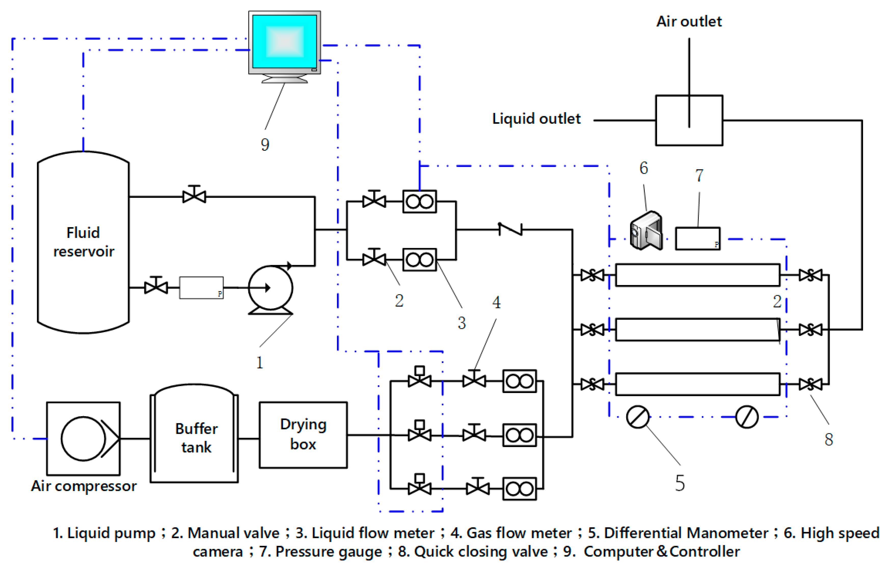
Figure 1: Laboratory setup diagram.
The experimental study on simulating the critical liquid-carrying state of gas-liquid two-phase flow was conducted in the Laboratory of Multiphase Pipe Flow, where the critical liquid loading state under conditions of different pipe diameters and different gas-liquid flow rates was observed. Water and air were used respectively to simulate the two-phase flow of wellbore produced water and natural gas. Under normal temperature and pressure conditions, the air density, air dynamic viscosity is
Experiments were conducted using organic glass tubes with inner diameters of 75 mm and 60 mm respectively. In indoor experiments, the length of the flow channel is 10 m, which ensures sufficient distribution of the flow pattern. The liquid film reversal was observed via a high-speed camera to determine the critical liquid loading state of gas flow carrying liquid, and the gas flow velocities under different liquid volume conditions were recorded. The experimental procedures are as follows: ① The liquid phase flows out of the buffer tank, passes through the plunger pump and liquid flowmeter, and then enters the liquid pipeline; ② Air passes through the compressor, buffer tank, and gas flowmeter, and then enters the gas pipeline; ③ The two phases (liquid and gas) are mixed in the mixer at the front end of the test pipeline to form a two-phase fluid, which then enters the test pipe section; ④ With the liquid phase flow rate fixed, the gas volume is adjusted from high to low. The liquid phase fallback state is determined by observing the transparent test pipe section via a high-speed camera, and the gas flow velocity at this moment is recorded as the critical liquid-carrying flow velocity under the corresponding liquid volume; ⑤ Adjust the liquid volume, pipeline inclination angle, and pipe diameter multiple times respectively, and repeat the above steps.
All pressure fluctuation parameters are collected and stored using the NI PCI-6220 64-bit multifunctional data acquisition card, with a data acquisition frequency of 200 Hz. The NI PCI-6220 data acquisition card is equipped with 8 differential, 16-bit resolution voltage-type analog input interfaces and 24 digital I/O interfaces. The analog sampling rate is 250 kS/s. After the system is turned on, the sensor output signal is converted into an industrial standard signal through the signal conditioning module, which is then transmitted to the AI port of the PCI-6220 and converted into a digital signal recognizable by the PC.
The distribution diagram of the gas-liquid two phases under the critical liquid loading state is shown below. In this state, both liquid droplets and liquid films exist simultaneously (Fig. 2).
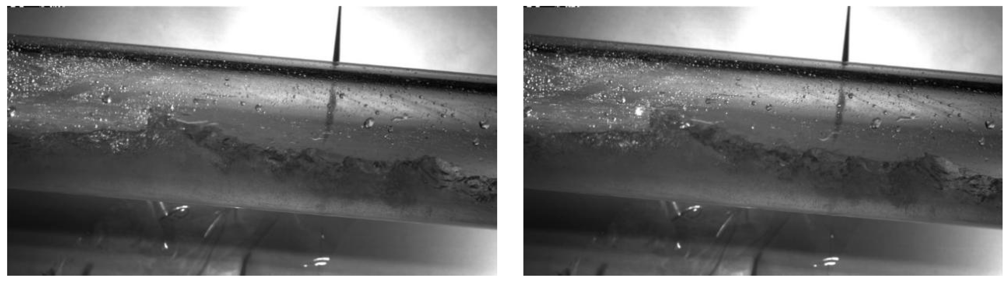
Figure 2: Distribution of gas-liquid two-phase flow under different liquid flow rates during critical liquid transport.
3 Analysis of Pressure Signals under the Critical Liquid Loading State
Since the critical liquid loading state of gas carrying liquid lies between slug flow and annular flow, this study focuses on monitoring the pressure fluctuations of slug flow and annular flow, aiming to capture and analyze the pressure signal characteristics corresponding to the critical liquid loading state in the transition zone between these two flow patterns. First, an analysis is conducted on the fluctuations of the gas-liquid two-phase flow pressure signals captured in the experiment under the slug flow state (Fig. 3):
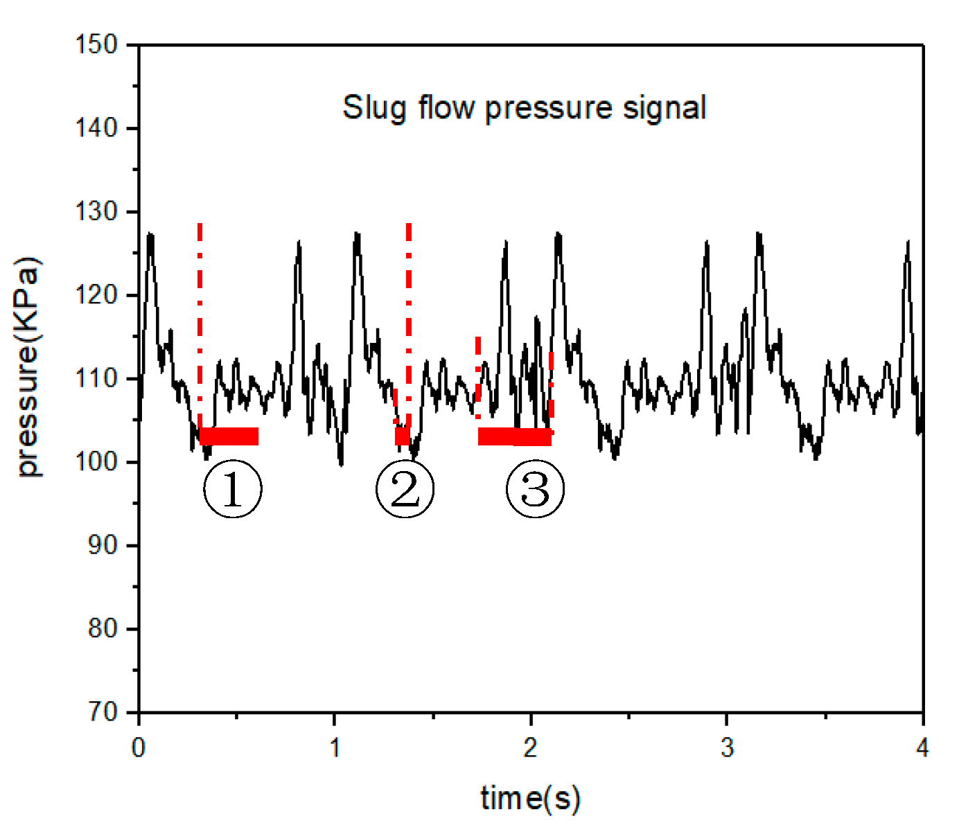
Figure 3: Slug flow pressure fluctuation signal.
The slug flow pattern exhibits strictly periodic motion, and the fluctuation amplitudes caused by the changes in its cycle period, liquid slug length, and liquid slug velocity over time are very small [10]. When slug flow occurs in the pipeline, the pressure fluctuation at the pressure measurement point is closely related to the movement position of the liquid slug. Since slug flow exhibits obvious regularity and periodicity during the flow process, the pressure fluctuation at the pressure measurement point will inevitably show periodic fluctuation as well. When gas enters the riser, causing the tail of the liquid slug to move away from the pressure measurement point, the pressure decreases rapidly (State ①). When the accumulated liquid phase blocks the pipeline, the subsequent gas expansion accelerates the accumulated liquid phase, which then passes through the pressure measurement point in one go—at this moment, the pressure at the pressure measurement point rises sharply (State ②). After the liquid phase passes through, a new round of liquid phase accumulation occurs at the bottom of the pipeline, and the pressure fluctuation remains stable for a period of time (State ③).
It can be seen from Fig. 4 that compared with slug flow, the pressure amplitude of annular flow during flow is smaller. The annular flow recorded in the experiment belongs to the early flow state of annular flow. The pressure at the pressure measurement point fluctuates slightly because the liquid ring climbs in a pulsed manner. Compared with slug flow, the pulsation frequency of the pressure signal is higher, while the pulsation amplitude is relatively smaller. Under the conditions of the same inclination angle and liquid production rate, it is easy to determine whether the gas-liquid two-phase flow in the pipeline is in the slug flow or annular flow stage through pressure fluctuations.
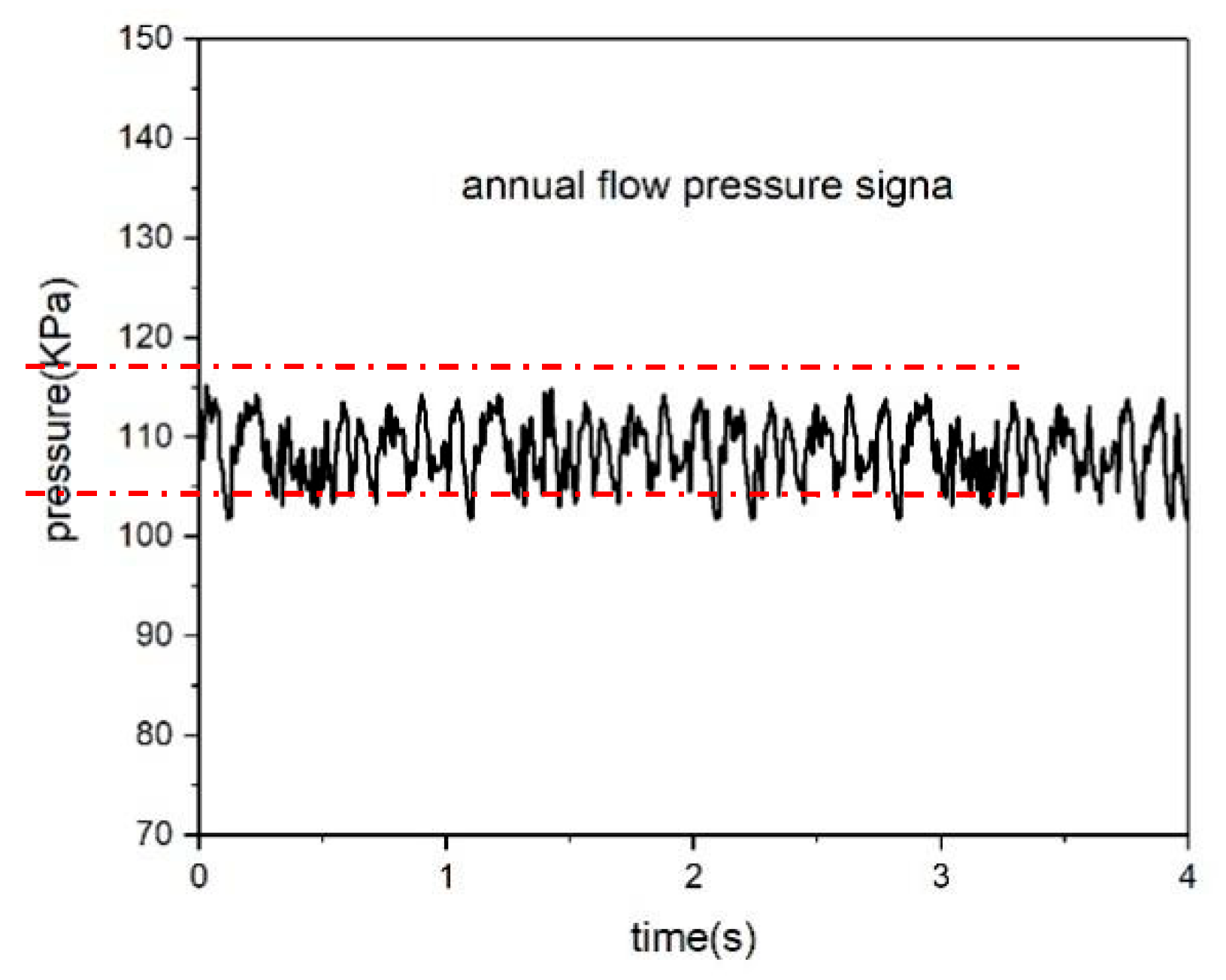
Figure 4: Annular flow pressure signal.
It can be seen from Fig. 5 that the pressure fluctuation in the critical liquid loading state neither has the periodicity of slug flow nor the stability of annular flow. Its pressure fluctuation is smaller than that of slug flow but larger than that of annular flow. Under the critical liquid loading state, as the liquid phase accumulates, occasional liquid phase surges may still form, and this is reflected in the pressure fluctuation as shown in ①. The pressure fluctuation in the critical liquid loading state does not require a long-term liquid phase accumulation process, which is a difference from slug flow (see ③ in Fig. 3). The reason is that the liquid phase in the critical liquid loading state does not experience large-scale fallback like that in slug flow; instead, it forms a local liquid seal at the pipe wall. As the liquid phase accumulates and the liquid phase in the gas core falls back, partial and non-intense liquid phase surges are formed. Although the formation of surges does not require liquid phase accumulation, the situation shown in ② of Fig. 5 may still occur. Different from slug flow, the liquid phase stability in the critical liquid loading state is not for accumulating liquid to form liquid slugs; instead, it is because the liquid phase is in a relatively static state—unable to be carried upward by the gas phase and unable to fall down due to the blowing of the gas phase. When the equilibrium point is disturbed and disrupted, the situation will return to that shown in ① of Fig. 5.
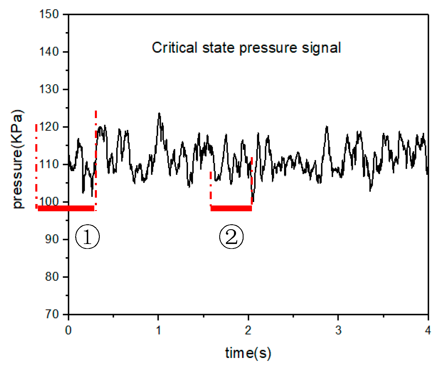
Figure 5: Pressure signal of critical liquid carrying state.
Through the monitoring and analysis of high-frequency pressure signals at the measurement points, different flow states exhibit different types of pressure signal fluctuations. To eliminate the subjectivity of the visual observation method in flow observation, it is objective and feasible to record and define the critical liquid loading state using pressure fluctuation signals. Obvious signal fluctuation patterns can be observed in Fig. 6, Fig. 7, Fig. 8 and Fig. 9, and the critical liquid loading state can be accurately defined by analyzing the regularity characteristics of pressure signals.
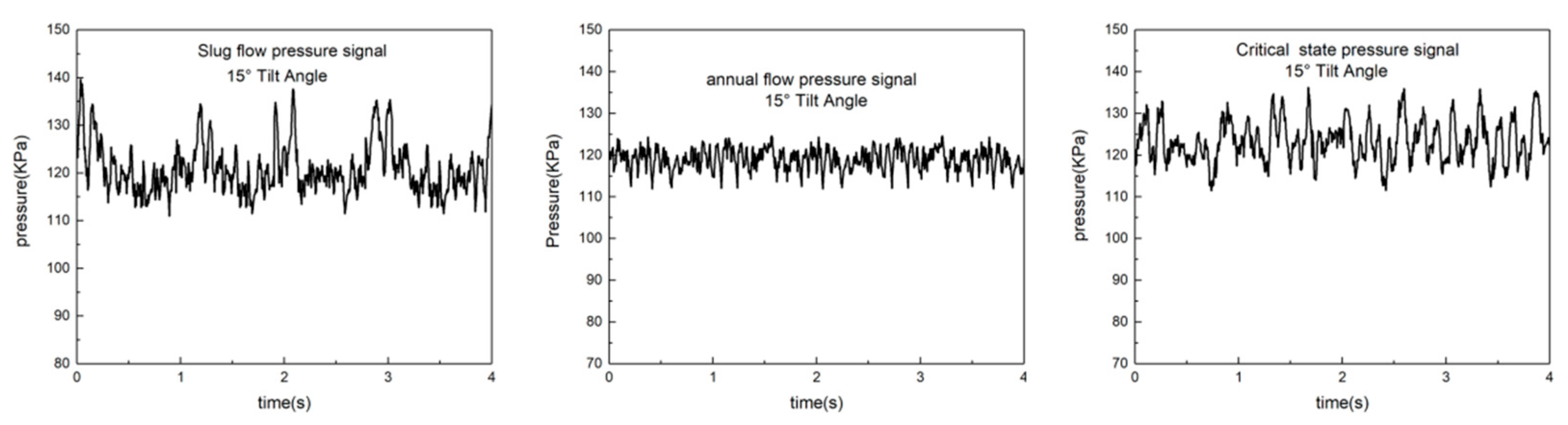
Figure 6: Comparison of pressure signals under different flow states with a tilt angle of 15°.
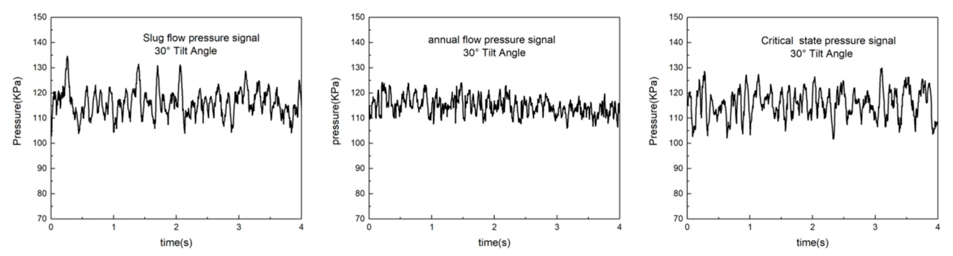
Figure 7: Comparison of pressure signals under different flow states with a tilt angle of 30°.
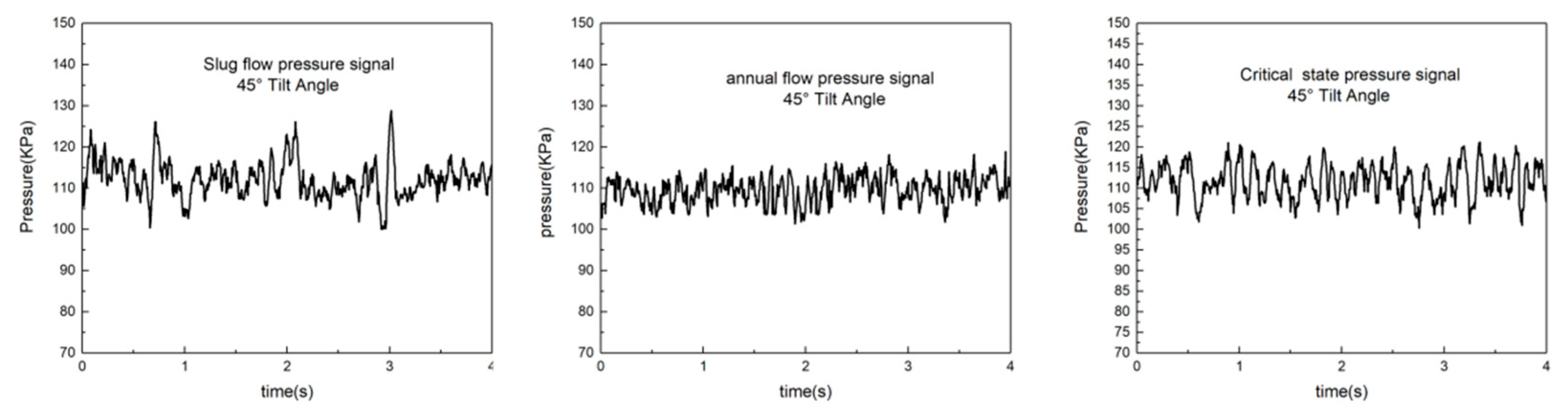
Figure 8: Comparison of pressure signals under different flow states with a tilt angle of 45°.
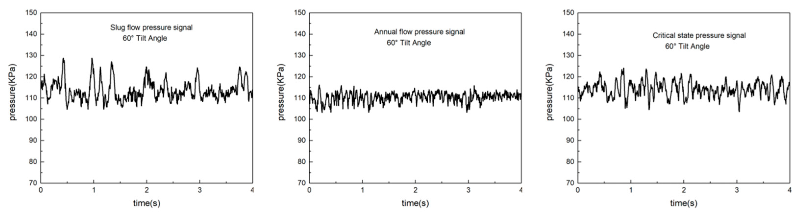
Figure 9: Comparison of pressure signals under different flow states with a tilt angle of 60°.
4 Processing of Pressure Signals under the Critical Liquid Loading State
It can be seen from Fig. 6 to Fig. 9 that there are significant differences in the pressure fluctuation signals under different flow states in the pipeline. From this, a conclusion can be drawn: if statistical parameters that are different from those under other gas-liquid carrying states and can characterize the flow pattern characteristics can be obtained from the pressure fluctuation signals [11,12,13], the flow pattern of the critical liquid loading state can be further identified.
To further analyze the high-frequency signals, this study adopts the Empirical Mode Decomposition (EMD) method [14] to convert the differential pressure fluctuation signals into single-frequency waves. This method can decompose the data sequence to be processed into a limited number of Intrinsic Mode Functions (IMF). Each IMF component obtained through the decomposition can effectively cover the local characteristics of the original time series at different scales [15]. The core idea of Empirical Mode Decomposition (EMD) is to convert a waveform with irregular frequency characteristics into a combination of multiple single-frequency waveforms and a residual waveform, i.e., Original Waveform =
Decomposition Process of EMD:
- (1)First, identify all the maximum points of the differential pressure fluctuation signal
- (2)Subtract the differential pressure signal from the curve
- (3)Repeat the above process k times, with the condition that
The screening-based processing method can obtain Intrinsic Mode Functions (IMFs) according to the different time scales of the signal, which facilitates signal analysis to achieve smooth amplitude and eliminate harmonics. To prevent the loss of data sequences, the number of screening iterations is limited, and the value of the standard deviation (SD) is used as the constraint condition for screening. The processing will terminate when the standard deviation reaches the set value; the SD used in this text is 0.1.
- (4)Remove the first Intrinsic Mode Function (IMF) component
The Empirical Mode Decomposition (EMD) algorithm itself has certain limitations, among which mode mixing is a key issue. When the EMD algorithm is applied to decompose signals, the mode mixing phenomenon can lead to two problems: oscillations with different time scales are incorrectly assigned to the same mode, or oscillations with similar time scales are scattered across different modes. This issue may be caused by abnormal phenomena such as random noise, interference, or signal interruptions in observations. The occurrence of mode mixing is mainly due to the fact that the envelope mean screening method used in the EMD process is affected by the distribution of local extreme points. The aforementioned uncontrollable conditions cause the distribution of local extreme points to deviate from their correct positions. Therefore, it is necessary to add Gaussian white noise to generate a new decomposition mode, which is called the Complementary Ensemble Empirical Mode Decomposition (CEEMD) [17]. The CEEMD algorithm makes full use of the characteristics of the EMD quadratic filter and effectively solves the EMD mode mixing problem:
- (1)During N decomposition experiments, the Gaussian white noise time series
Among them, N represents the number of times the data sequence undergoes Empirical Mode Decomposition.
- (2)Decompose time series A and B using the EMD algorithm program.
Among them, M represents the total number of Intrinsic Mode Functions (IMFs) obtained after the n-th Empirical Mode Decomposition;
- (3)Repeat Steps 1 and 2 for N times. Each time the decomposition is performed, the randomly generated Gaussian white noise will form a new data sequence together with the original data.
- (4)Utilizing the zero-mean statistical property of noise, calculate the averages of the Intrinsic Mode Function (IMF) groups
After decomposition by the Complementary Ensemble Empirical Mode Decomposition (CEEMD), the original differential pressure signal can also be expressed in the following form:
An analysis of the above decomposition steps reveals that the CEEMD decomposition results are closely associated with two key factors: the number of ensembles (N) of Gaussian white noise and the amplitude (A) of the superimposed Gaussian white noise. The number of ensembles (N) of Gaussian white noise in the original signal shall satisfy the following formula:
Among them, A is the standard deviation (SD), and the recommended value of N is 100. Studies have shown that good results can be achieved when the amplitude of the added noise is a fraction of the standard deviation of the original data; therefore, the amplitude of the added noise in this paper is set to 0.2.
Taking the high-frequency pressure signals of gas-liquid two-phase flow with a pipe diameter of 60 mm and flow angles of 60° and 90° as examples, the differential pressure signals after CEEMD decomposition are shown in Fig. 10, Fig. 11, Fig. 12, Fig. 13, Fig. 14 and Fig. 15.
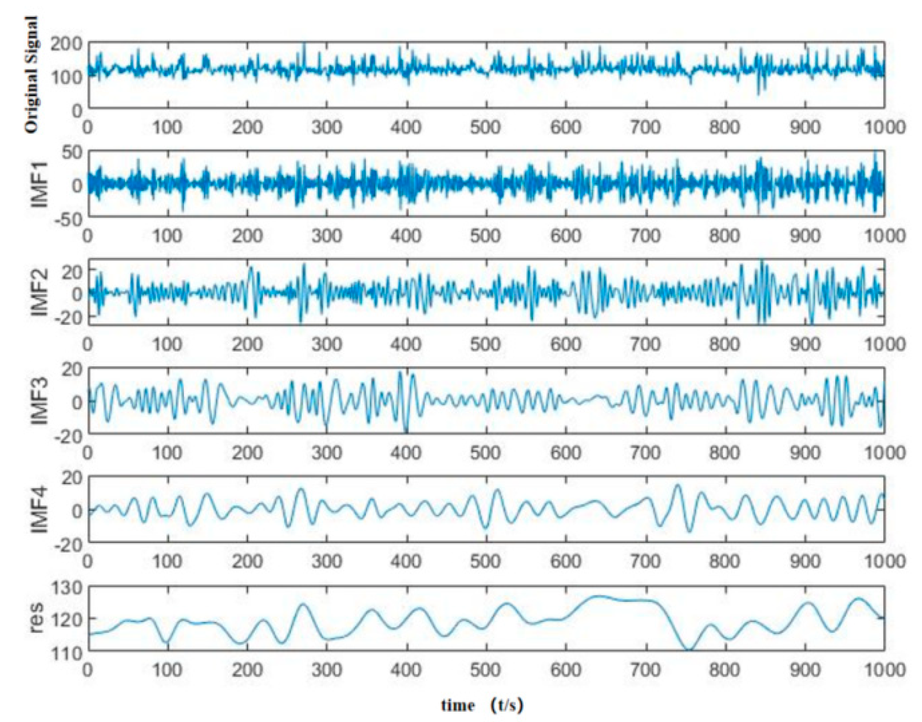
Figure 10: Blocking flow during a 60° period with a 60 mm pipe diameter.
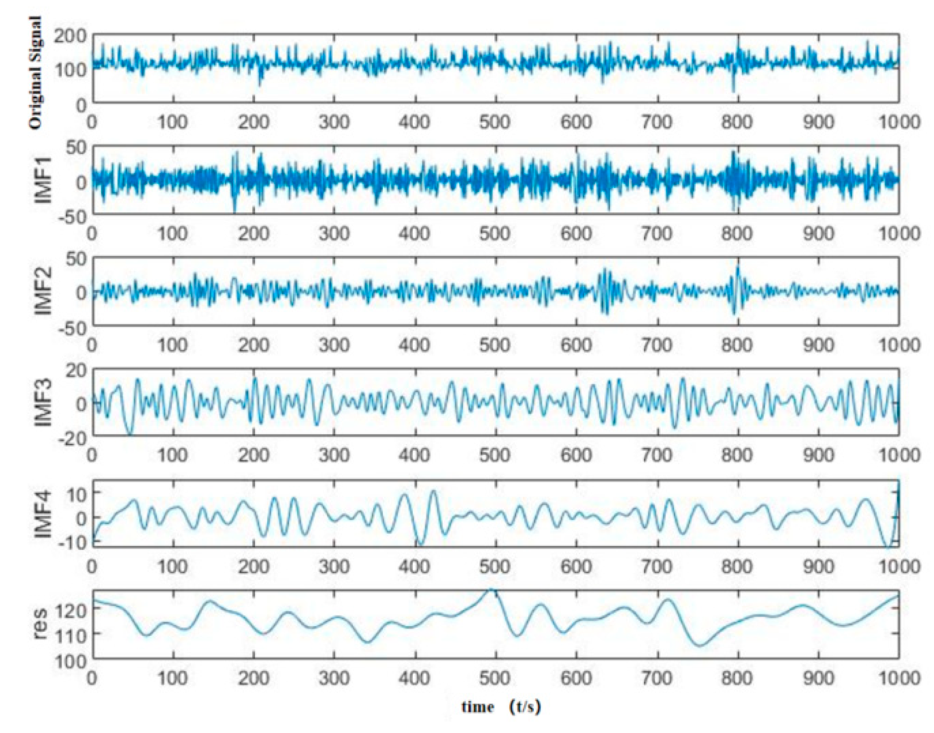
Figure 11: Annular flow with a 60 mm pipe diameter of 60°.
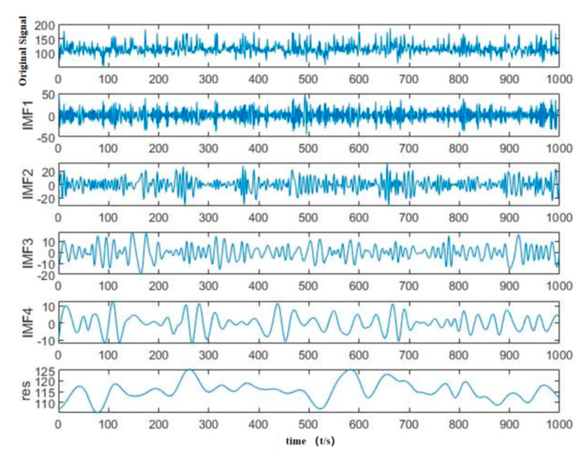
Figure 12: Critical liquid carrying flow rate at 60° for a 60 mm pipe diameter.
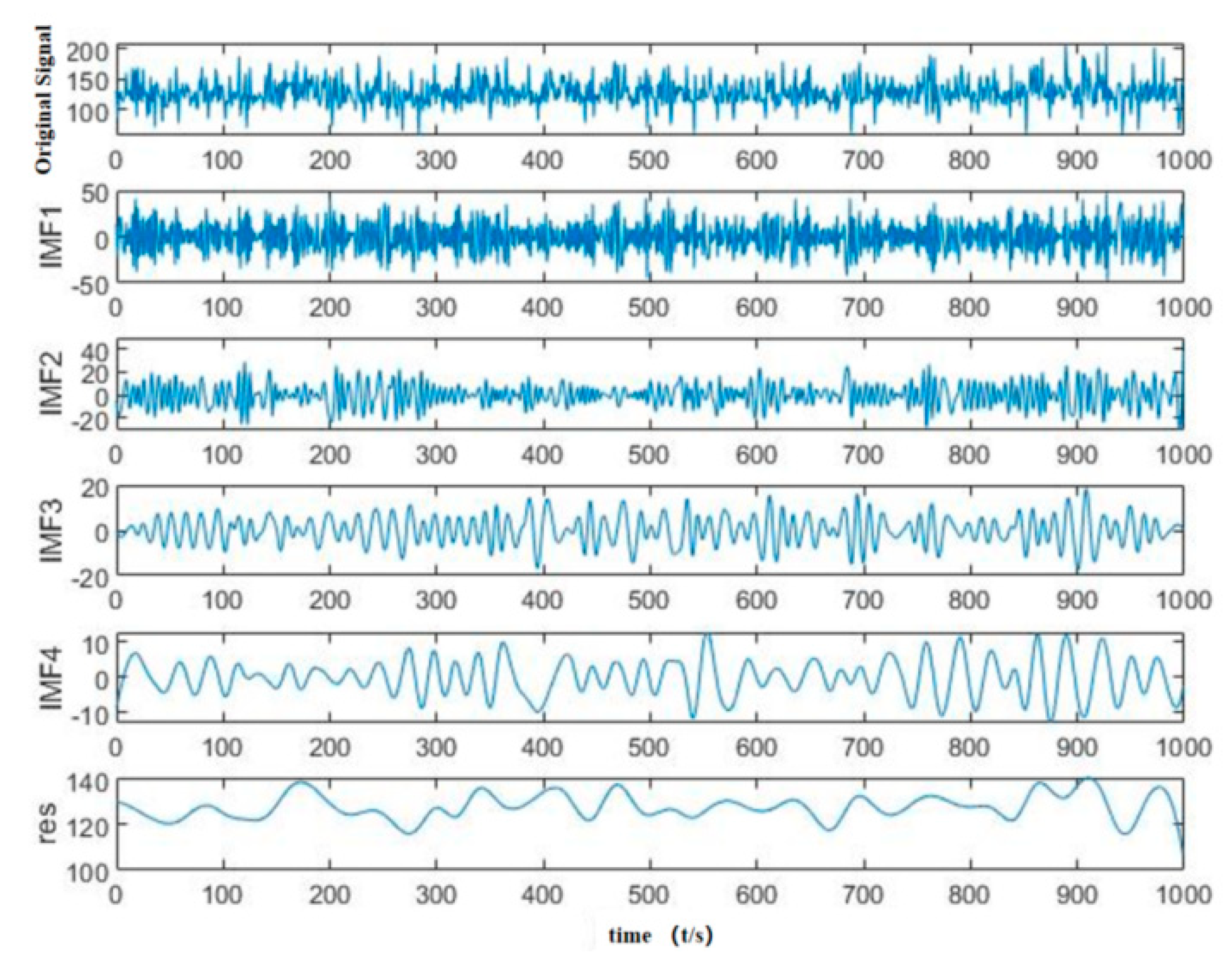
Figure 13: Slug flow at a 60 mm pipe diameter of 90°.

Figure 14: Annular flow with a 60 mm pipe diameter of 90°.
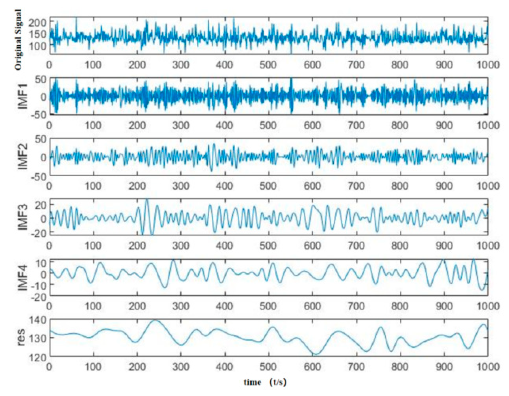
Figure 15: Critical liquid carrying capacity at 90° for a 60 mm pipe diameter.
The obtained new data sequence is expressed in the following form:
To characterize the features of slug flow, annular flow, and critical liquid-carrying states, this study combines statistical and fractal theories to extract flow pattern characteristic parameters. Specifically, the original pressure fluctuation signal is decomposed using the Complementary Ensemble Empirical Mode Decomposition (CEEMD) algorithm, and 4 Intrinsic Mode Function (IMF) components are screened out. Then, their energy entropy, kurtosis coefficient, and variance are used as statistical parameters to realize the objective identification of the critical liquid-carrying state in the transition region between slug flow and annular flow (Fig. 16, Fig. 17 and Fig. 18).
- (1)Variance
Variance [13] can reflect the concentration range of fluctuations in the differential pressure signal under gas-liquid two-phase flow conditions. Different flow patterns exhibit varying degrees of fluctuation, and their variances also differ accordingly. Through pressure signal analysis, the variance range of the critical liquid-carrying state fluctuates between 0.64 and 0.86, the variance of the annular flow signal fluctuates within the range of 0.38 to 0.46, and the variance range of the pressure signal in the slug flow state fluctuates between 1.3 and 1.45.
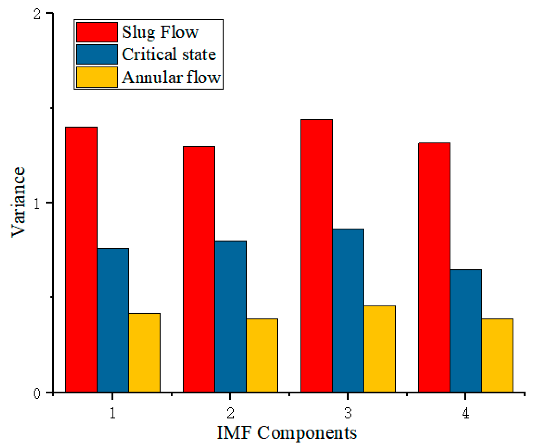
Figure 16: Variance distribution of different IMF components under different flow states.
- (2)IMF Energy Entropy
Perform CEEMD decomposition on the original signal, and calculate the energy
The total energy
Calculate the proportion of each energy component to the total energy
The energy entropy is:
Verification through a large amount of experimental data shows that the critical liquid-carrying state can be easily distinguished by selecting the energy of each IMF [18,19]. Partial data are shown in Table 1; the energy of the critical liquid-carrying signal is much greater than that of other signals:
Table 1: Energy entropy table of pressure signals for each layer after CEEMD decomposition.
| C1 | C2 | C3 | C4 | |
|---|---|---|---|---|
| Slug Flow 1 | 1.0676 | 0.7212 | 0.2697 | 0.1281 |
| Slug Flow 2 | 1.2521 | 0.8266 | 0.31 | 0.1296 |
| Annular flow 1 | 0.6335 | 0.3655 | 0.1467 | 0.0354 |
| Annular flow 2 | 1.1349 | 0.6917 | 0.2948 | 0.1274 |
| Critical state 1 | 1.2042 | 0.7586 | 0.3247 | 0.1628 |
| Critical state 2 | 1.2523 | 0.8285 | 0.3101 | 0.1301 |
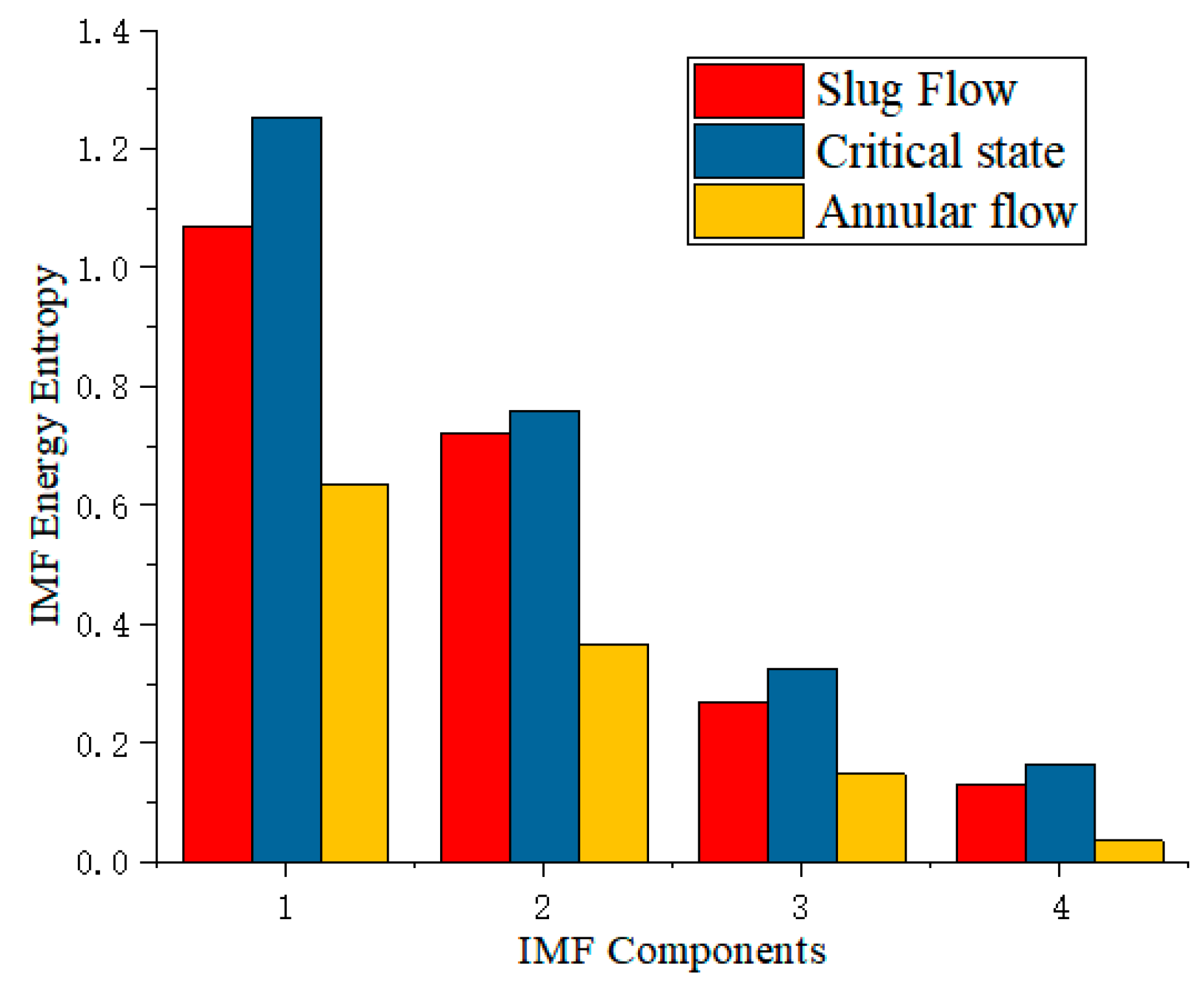
Figure 17: Distribution of energy entropy of different IMF components under different flow states.
- (3)Kurtosis Coefficient
The kurtosis coefficient reflects the degree to which the distribution of a pressure fluctuation signal approximates a normal distribution [20,21].
The calculation of the kurtosis coefficient is as follows:
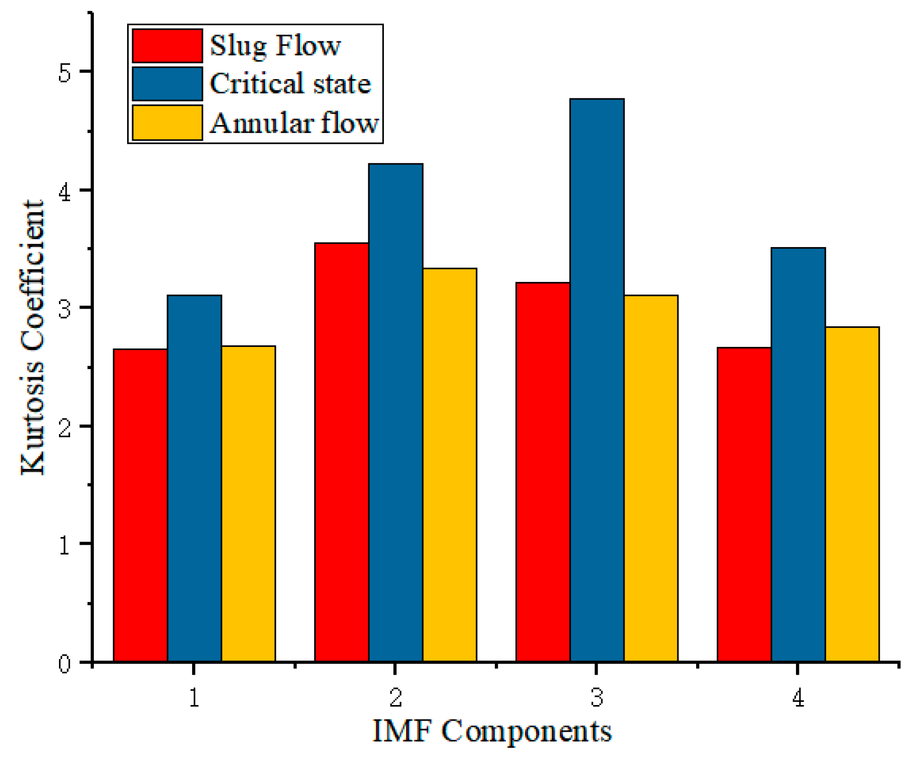
Figure 18: Kurtosis coefficients of different IMF components under different flow states.
It can be observed from the above figures that the kurtosis coefficient under the critical liquid loading state is significantly higher than that under slug flow and annular flow. Therefore, the distribution characteristics of the kurtosis coefficient of pressure fluctuation signals vary greatly: the kurtosis coefficient distribution range is 2.67–3.5 for slug flow, 2.73–3.35 for annular flow, and 3.13–4.68 for the critical liquid-carrying state. This characteristic parameter can be used to distinguish the critical liquid loading state of gas-liquid carrying.
In summary, the feature quantities and identification method adopted in this paper are reasonable and effective. When the number of samples is sufficient, through the analysis of pressure fluctuation signals, the use of appropriate feature quantities and identification methods can effectively achieve objective identification of the critical liquid-carrying state, avoiding the subjective drawback of the visual observation method.
This article proposes a quantitative discrimination criterion based on high-frequency pressure signal analysis through in-depth research on the critical liquid loading state of gas-liquid entrainment, effectively solving the problems of inconsistent quantitative standards and strong subjectivity in traditional methods. The experimental results indicate that the critical liquid carrying state is located between slug flow and annular flow, and exhibits specific pressure fluctuation characteristics. By using Empirical Mode Decomposition (EMD) and Complementary Ensemble Empirical Mode Decomposition (CEEMD) methods to process pressure signals, statistical measures such as variance, IMF energy entropy, and kurtosis coefficient were extracted to characterize different flow patterns. These feature quantities show significant differences between slug flow, annular flow, and the critical carrier state, which can effectively distinguish and identify the critical liquid loading state. The main contribution of this article is to propose a quantitative judgment method that can objectively identify the critical liquid carrying state. Although current research is limited by the scale of experimental data, the accuracy and universality of this judgment method can be further improved by incorporating more experimental data under different operating conditions in the future. This method can be further combined with machine learning, based on large-scale datasets and integrating high-frequency signal reception technology, to develop into a stable intelligent recognition system for critical liquid carrying states. This study provides important theoretical basis and experimental evidence for establishing a more accurate critical fluid carrying model, which is of great significance for guiding the judgment of gas well fluid accumulation and optimizing oil and gas production.
Acknowledgement:
Funding Statement: The authors received no specific funding for this study.
Author Contributions: The authors confirm contribution to the paper as follows: Yang Cheng: Conceptualization; Methodology; Writing—Original draft preparation; Writing—Original draft preparation. Zhiyang Sun: Writing—Original draft preparation; Funding acquisition; Project administration; Software; Validation. Dajiang Wang: Data curation; Software; Validation; Data curation;Funding acquisition. All authors reviewed and approved the final version of the manuscript.
Availability of Data and Materials: The data that support the findings of this study are available from the Corresponding Author, [Yang Cheng], upon reasonable request.
Ethics Approval: Not applicable.
Conflicts of Interest: The authors declare no conflicts of interest.
References
1. Tang Y , Tang X , Wang GY , Zhang Q . Summary of hydraulic fracturing technology in shale gas development. Geol Bull China. 2011; 30( 2/3): 393– 9. (In Chinese). [Google Scholar]
2. Gomez Camperos JA , Hernández Cely MM , Pardo García A . Artificial intelligence techniques for the hydrodynamic characterization of two-phase liquid–gas flows: An overview and bibliometric analysis. Fluids. 2024; 9( 7): 158. doi:10.3390/fluids9070158. [Google Scholar] [CrossRef]
3. Liu S , Wang X , Li L , Feng J , Liao R , Wang X . Critical liquid-carrying model for horizontal gas well. Int J Heat Technol. 2018; 36( 4): 1304– 9. doi:10.18280/ijht.360419. [Google Scholar] [CrossRef]
4. Turner RG , Hubbard MG , Dukler AE . Analysis and prediction of minimum flow rate for the continuous removal of liquids from gas wells. J Petrol Technol. 1969; 21( 11): 1475– 82. doi:10.2118/2198-pa. [Google Scholar] [CrossRef]
5. Coleman SB , Clay HB , McCurdy DG , Norris LH III . A new look at predicting gas-well load-up. J Petrol Technol. 1991; 43( 3): 329– 33. doi:10.2118/20280-pa. [Google Scholar] [CrossRef]
6. Zheng J , Li J , Dou Y , Zhang Y , Yang X , Zhang Y . Research progress on the calculation model of critical liquid carrying flow of gas well. Energy Sci Eng. 2023; 11( 12): 4774– 86. doi:10.1002/ese3.1601. [Google Scholar] [CrossRef]
7. Liu Y , Liu X , Luo C , Long H , Li F , Luo J , et al. Establishment and experimental verification of the evaluation method for the dynamic liquid-carrying performance of foaming agents based on correlation analysis. Ind Eng Chem Res. 2025; 64( 8): 4260– 71. doi:10.1021/acs.iecr.4c04498. [Google Scholar] [CrossRef]
8. Luo S . New comprehensive equation to predict liquid loading. In: Proceedings of the SPE Annual Technical Conference and Exhibition; 2013 Sep 30–Oct 2; New Orleans, LA, USA. doi:10.2118/167636-stu. [Google Scholar] [CrossRef]
9. Minchenkov ND , Churakova SK . Development of an improved calculation method for hollow horizontal gas-liquid separators. Theor Found Chem Eng. 2025; 59( 3): 677– 81. doi:10.1134/S0040579525602158. [Google Scholar] [CrossRef]
10. Muñoz-Cobo JL , Chiva S , Ali Abd El Aziz Essa M , Mendes S . Simulation of bubbly flow in vertical pipes by coupling Lagrangian and Eulerian models with 3D random walks models: Validation with experimental data using multi-sensor conductivity probes and Laser Doppler Anemometry. Nucl Eng Des. 2012; 242: 285– 99. doi:10.1016/j.nucengdes.2011.10.021. [Google Scholar] [CrossRef]
11. Li J , He K , Tan M , Cheng X . An adaptive CEEMD-ANN algorithm and its application in pneumatic conveying flow pattern identification. Flow Meas Instrum. 2021; 77: 101860. doi:10.1016/j.flowmeasinst.2020.101860. [Google Scholar] [CrossRef]
12. Camargo TFB , Paladino EE . Characterization of transient differential pressure signal features and flow pattern identification in horizontal two-phase flow through a constriction with machine learning models. Flow Meas Instrum. 2025; 106: 102985. doi:10.1016/j.flowmeasinst.2025.102985. [Google Scholar] [CrossRef]
13. Khan U , Pao W , Pilario KES , Sallih N , Khan MR . Two-phase flow regime identification using multi-method feature extraction and explainable kernel Fisher discriminant analysis. Int J Numer Meth Heat Fluid Flow. 2024; 34( 8): 2836– 64. doi:10.1108/hff-09-2023-0526. [Google Scholar] [CrossRef]
14. Singh S , Lalotra S , Sharma S . Dual concepts in fuzzy theory: Entropy and knowledge measure. Int J Intell Syst. 2019; 34( 5): 1034– 59. doi:10.1002/int.22085. [Google Scholar] [CrossRef]
15. Rhif M , Ben Abbes A , Farah IR , Martínez B , Sang Y . Wavelet transform application for/in non-stationary time-series analysis: A review. Appl Sci. 2019; 9( 7): 1345. doi:10.3390/app9071345. [Google Scholar] [CrossRef]
16. Zhou H , Ding J , Lin C , Li XQ . Denoising method based on secondary CEEMD and time domain feature analysis. J Electron Meas Instrum. 2023; 37( 3): 222– 9. (In Chinese). [Google Scholar]
17. Li ZJ , Zhang HP , Wang YN , Li X . Wavelet threshold denoising harmonic detection method based on permutation entropy-CEEMD decomposition. Electr Mach Control. 2020; 24( 12): 120– 9. (In Chinese). [Google Scholar]
18. Mercante R , Netto TA . Virtual meter with flow pattern recognition using deep learning neural networks: Experiments and analyses. SPE J. 2024; 29( 5): 2181– 96. doi:10.2118/219465-pa. [Google Scholar] [CrossRef]
19. Mayet AM , Mohammed SA , Gorelkina EI , Hanus R , Guerrero JWG , Qamar S , et al. Correction: MLP ANN equipped approach to measuring scale layer in oil-gas-water homogeneous fluid by capacitive and photon attenuation sensors. J Nondestruct Eval. 2025; 44( 3): 111. doi:10.1007/s10921-025-01237-2. [Google Scholar] [CrossRef]
20. Shakarami R , Sadeghi MT . Gas-liquid two-phase flow measurement based on emitted acoustic signal anomaly and deep learning approach. Flow Meas Instrum. 2026; 107: 103097. doi:10.1016/j.flowmeasinst.2025.103097. [Google Scholar] [CrossRef]
21. Sun B . The identification method of gas-liquid two-phase flow regime based on wavelet and chaos theory. Beijing, China: North China Electric Power University; 2005. p. 50– 67. (In Chinese). [Google Scholar]
Cite This Article
 Copyright © 2026 The Author(s). Published by Tech Science Press.
This work is licensed under a Creative Commons Attribution 4.0 International License , which permits unrestricted use, distribution, and reproduction in any medium, provided the original work is properly cited.
 Downloads
 Citation Tools