Integrated Mechanistic Analysis and Machine Learning Prediction of Slug Flow in Oil-Gas-Water Three-Phase Pipelines

1 Introduction

Slug flow is a classic challenge in the field of multiphase flow transportation. As the energy industry advances toward more complex and harsh environments, this challenge becomes increasingly prominent. This unstable flow pattern can induce severe pipeline vibration, significant fluctuations in system pressure, and impacts on terminal processing equipment, severely restricting the safety and operational efficiency of production systems.

Currently, some researchers have obtained a series of study outcomes in the formation mechanism of slug flow. The development of slug flow starts with the strengthening of instabilities inside the liquid film. These instabilities usually manifest as interfacial waves, which grow in amplitude until they span the pipe cross-section [1]. Under specific conditions, however, these waves may not reach sufficient height to reach the pipe crown, leading to the creation of pseudo-slug structures. These appear as large-amplitude waves that partially block the pipe’s internal cross-section and move at a speed lower than the translational speed of a fully developed slug [2,3]. After formation, slug flow shows a cyclical pattern: in low-pressure zones, a developing slug moves at high speed, sweeping up the liquid ahead. This creates a hydrostatic imbalance and eventually leads to the collapse of the liquid bridge downstream. This collapse, in turn, generates new disturbances that trigger the next slug in the cycle. Slugs expand by interacting with the leftover liquid film shape left by prior slugs, eventually reaching a quasi-steady state where the rates of liquid entrainment and shedding are balanced. If the liquid height drops below the critical limit needed to maintain a slug, the structure starts to break down the process elaborated by Taitel et al. [4], Davies et al. [5], and Barnea et al. [6].

To study the factors that affects the slug flow, Ma et al. [7] used FLUENT to conduct three-dimensional simulations of liquid slugs and annular flows at different velocities in gas-liquid dual-phase flow within elbows, aiming to assess the elements affecting slug flow onset in such dual-phase flow inside elbows. Li et al. [8] conducted numerical simulations of gas-liquid dual-phase flow in DN50 pipelines using the Volume of Fluid (VOF) method paired with adaptive dynamic grid techniques. The reliability of the CFD simulation was validated by cross-referencing with experimental datasets and literature results, with in-depth analysis conducted on the influence mechanisms of various factors. Lyu [9] obtained through computational simulations of two-phase gas-liquid flow that slug flow often occurs at locations where the pipeline layout changes, especially when a downward-inclined pipeline connects to a vertical riser, which is prone to inducing severe slug flow. Dang et al. [10] illustrated through research on two-phase gas-liquid flow that the influencing factors of severe slug flow include flow velocity and gas flow rate, and proposed methods to effectively reduce severe slug flow in riser sections. Ren et al. [11] conducted an in-depth investigation into the characteristics of gas-liquid dual-phase flow in horizontal pipes and uncovered how varying gas-liquid flow ratios impact the initiation of slug flow. Wang et al. [12] centered their research on examining, through experiments, how changes in the tilt angle of gas-liquid dual-phase flow pipelines affect the flow pattern transition boundary.

To simulate the slug flow accurately, the study of the slug tracking model has undergone a long period of development [13,14]. The slug tracking model has been improved in different ways. Nydal et al. [15] extended this mathematical framework to pipelines with variable tilt angles, establishing mass balance equations for the liquid slug (under the assumption of no gas), the elongated bubble, and the transient liquid film. Many scholars [16,17,18] centered their research on inclined pipelines, integrating temperature fluctuations and introducing pressure differences described via momentum flux to capture head losses caused by liquid recirculation in the wake of the elongated bubble. Smoothed Particle Hydrodynamics (SPH), as a Lagrangian particle-based method, is inherently well-suited for simulating flows involving large deformations, free surfaces, and complex interfaces. For instance, the smoothed-interface SPH model for multiphase fluid-structure interaction developed by Guo et al. [19,20] is used to accurately capture interactions at phase interfaces. This provides a new paradigm for studying the dynamic response of pipe walls under slug impact loads. For slug flow, three classic modeling approaches are available: the cell-averaged model, the slug tracking method, and the slug capture method. Nevertheless, the precision and reliability of the slug capture model largely depend on grid resolution, leading to substantial consumption of computational resources and time. Thus, it is crucial to propose an efficient and precise approach for slug flow prediction [21,22].

However, existing studies mainly focus on two-phase flow or specific operating conditions [23,24], and the formation mechanism of slug flow in oil-gas-water three-phase flow has not been fully clarified, nor have the various factors affecting slug flow formation been comprehensively summarized and analyzed. Compared with two-phase flow, the flow patterns of oil-gas-water three-phase flow exhibit more complex spatiotemporal inhomogeneous distribution characteristics. Currently, some researchers have carried out relevant theoretical and experimental studies focusing on the flow characteristics of different three-phase flow patterns and the transition properties between these patterns. For example, Açıkgöz et al. [25] conducted dynamic experimental observations on oil-gas-water three-phase flow in horizontal pipelines by setting up a transparent observation window, and proposed a three-element method for defining the types of three-phase flow patterns based on the observation results. The first element is to determine the continuous phase (oil-based or water-based) according to the relationship between the liquid phase and the pipe wall; the second element is to identify the flow structure between the two liquid phases (separated or dispersed); the third element is to confirm the flow structure between the gas and liquid phases (bubbly, stratified, wavy, plug, slug, or annular flow). This method has laid an important foundation for subsequent research on the flow patterns and identification of oil-gas-water three-phase flow. Wegmann et al. [26] defined oil-gas-water three-phase flow patterns by combining the gas-liquid interfacial structure and the oil-water interfacial structure, and measured the oil-gas-water three-phase flow in small-diameter horizontal pipelines using high-speed cameras and laser-induced fluorescence (LIF) technology, revealing the flow characteristics of six flow patterns (stratified-intermittent flow, annular-intermittent flow, intermittent-dispersed flow, intermittent-intermittent flow, dispersed-intermittent flow, and dispersed-annular flow). Due to differences in experimental conditions, there are certain discrepancies in the conclusions drawn by different researchers. To date, universal standards for the definition, transition, and classification of oil-gas-water three-phase flow patterns have not been established, and relevant research is still in the developmental stage. The accurate identification of oil-gas-water three-phase flow patterns still faces tremendous difficulties and challenges.

To this end, this paper develops a high-fidelity oil-gas-water three-phase flow model to systematically unravel the slug flow formation mechanism, addressing the issue that the model is difficult to apply to the real-time and rapid prediction of on-site slug flow conditions, this paper selects the optimal model for slug flow prediction by comparing the applicability of different machine learning models, and establishes an efficient machine learning prediction model. This research not only deepens the understanding of the mechanism but also provides a key technical tool for realizing intelligent monitoring of pipelines and rapid scheme screening. In contrast to the majority of current research focused on gas-liquid dual-phase flow, the slug flow prediction is comparatively sluggish and imprecise. This study mainly explores the emergence of slug flow in pipelines carrying high-viscosity crude oil blended with associated gas and water, and conducts comparisons among various machine learning models. The research pinpoints the machine learning model featuring optimal predictive capability, enabling the efficient and precise determination of slug flow formation.

2 Analysis of Influencing Factors and the Mechanism Underlying Slug Flow Formation

The formation of slug flow is the result of the strong coupling of multiple factors such as thermodynamic conditions, fluid composition, and pipeline geometric characteristics. By reviewing literature, this study identifies temperature, gas-liquid ratio, liquid flow rate, water cut, and pipeline inclination angle as core influencing factors. The regulatory effects of each factor are explored by assessing variations in gas superficial velocity, liquid velocity, liquid phase viscosity, liquid surface tension, and the axial component of gravity: higher system temperature, higher volume water cut, lower liquid phase flow rate, higher gas-liquid ratio, and larger pipeline inclination angle all significantly enhance flow instability, thereby promoting the formation and development of slug flow. The specific influence laws are shown in Fig. 1, where red represents liquid slugs, brown represents liquid, and blue-white represents gas.

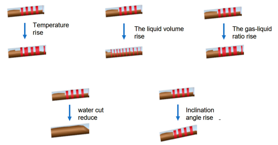
Figure 1: Development laws of slug flow under different factor changes.

The internal physical mechanism is elaborated as follows:

• (1)When the temperature rises, the liquid phase viscosity decreases, which strengthens the gas-phase’s shear disturbance on the liquid phase, accelerates the unstable growth of liquid surface fluctuations, and makes it easier to form slug flow;
• (2)When the total liquid flow rate decreases, the liquid film at the bottom of the pipeline becomes thinner and less continuous, and the surface tension of the liquid decreases, providing a penetration channel for the gas phase and promoting the formation of liquid slugs;
• (3)When the water cut rises, the liquid phase viscosity decreases, and the fluid mobility rises, which supports the formation of more stable, long-lasting liquid slugs;
• (4)When the gas-liquid ratio rises, the gas superficial velocity rises, the gas kinetic energy enhances, the entrainment and the gas phase’s ability to entrain and carry the liquid phase, making it easier to stir the liquid surface and form continuously moving liquid slug sections;
• (5)When the pipeline upward inclination angle rises, the liquid flow velocity decreases, and the axial component of gravity promotes the liquid phase to accumulate more easily in low-lying or climbing sections, causing local blockages, thereby triggering slug flow.

As illustrated in Fig. 2, the underlying physical mechanisms by which slug flow influencing factors act.

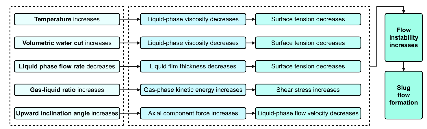
Figure 2: Influencing factors and variation trends of slug flow.

The above five factors jointly affect the formation of slug flow, so these five factors need to be considered when predicting slug flow formation.

3 Construction of Pipeline Oil-Gas-Water Three-Phase Flow Model

Among numerous multiphase flow simulation tools, OLGA has become the industry’s first choice owing to its strong capability to accommodate complex pipeline layouts and transient flow regimes [27]. Its model is based on solid multiphase flow theory and has been calibrated with a large amount of experimental and field data, especially in simulating complex conditions such as undulating pipelines and large-inclination wellbores with high accuracy. Through OLGA simulation, the dynamic response of the pipeline system under various operating conditions can be reliably obtained, including but not limited to pressure distribution, thermal changes, and flow pattern transitions. These detailed data provide a core basis for accurately analyzing flow laws. OLGA software serves as the data source for this study, despite its inherent limitations. Its underlying assumption relies on one-dimensional cross-sectional averaging, which hinders its ability to resolve three-dimensional flow details inside the pipeline’s cross-section. Several alternative software tools are available, including LedaFlow. Nevertheless, in OLGA’s slug tracking model, slug flow does not demand a fine mesh and can be simulated using a relatively coarse grid (with lengths equivalent to dozens of pipe diameters), thereby enabling a comparatively short simulation duration. In contrast, LedaFlow [28] solves waves and slugs directly on the computational grid through high-order numerical methods, necessitating a relatively fine mesh. Such a fine mesh, though, extends the computation time. Additionally, under specific extreme operating conditions, LedaFlow’s simulation results may fail to converge. At present, there are no effective solutions within LedaFlow to address this issue, leading this study to select OLGA as the simulation tool. For the OLGA software, there are three classic approaches for modeling slug flow including the unit cell model, slug tracking method, and slug capture method. The unit cell model is grounded in the principle of control volume averaging, making it well-suited for predicting the steady-state or statistically averaged behaviors of slug flow. By contrast, the slug tracking method adopts a Lagrangian framework, which treats each slug as a discrete entity and dynamically tracks its motion along the pipeline. Both the slug tracking and slug capture methods can provide the spatiotemporal distribution data required for the analysis of curved pipeline structures. Nevertheless, the accuracy and reliability of the slug capture method are highly dependent on grid resolution, which inevitably incurs substantial computational resources and time overheads. This thus underscores the imperative of developing a rapid and high-accuracy approach for slug flow prediction.

The construction of OLGA’s multiphase flow model includes the construction of physical property files and pipeline physical models.

OLGA incorporates three flow regime transition models: the Taitel-Dukler model [29], the Beggs-Brill model [30], and the modified Baker model [31]. The Taitel-Dukler model is well-suited for simulating low-viscosity oil-gas-water three-phase flow in horizontal or slightly inclined pipes; the Beggs-Brill model is applicable to simulating mixed fluids of medium-viscosity crude oil, associated gas, and water in pipelines at any angle of inclination; and the modified Baker model is designed for simulating high-viscosity crude oil flow in vertical or steeply inclined pipes. For distinct fluid types and pipeline configurations, the respective applicable empirical formulas are employed to compute the critical thresholds governing flow pattern transitions. If the actual gas-phase velocity surpasses the critical gas velocity, the flow pattern shifts from stratified flow to wavy stratified flow. If the liquid level exceeds the critical liquid height, the flow pattern transitions from wavy stratified flow to slug flow. If the liquid holdup surpasses its critical value, the flow pattern converts from stratified flow to bubbly flow.

The construction of physical property files usually uses Multiflash or PVTsim software. The workflow of both starts with defining a detailed list of fluid components in the software. Users can input detailed hydrocarbon components from C1 to C80+ and specify non-hydrocarbon components and water salinity. The software can select thermodynamic models, including cubic equations of state and advanced equations of state. When gums and asphaltenes are present, the asphaltene viscosity model should be selected to correct the viscosity and density of the mixture. Then, the temperature and pressure ranges as well as the oil-gas-water proportioning are determined. Finally, the phase equilibrium and physical property parameters of the fluid under different pressures and temperatures are calculated, and a physical property file directly callable by OLGA is generated. Both can well construct common fluid physical property files, and this study selects Multiflash to construct the physical property file.

Import the previously generated physical property file into the OLGA model. A simple physical model usually includes units such as inlet, outlet, pipeline, and valve. The inlet and outlet can set temperature and pressure as boundary conditions or temperature and flow rate as boundary conditions. The parameters to be set for the pipeline segment unit include length, elevation change, inner diameter, absolute roughness, pipe wall material, ambient temperature, and total heat transfer coefficient; the valve can set valve opening, valve position, and valve characteristics. The physical model established in OLGA is shown in Fig. 3. When there is a large amount of water in the fluid, the SteamWater-HC function should be used. Enabling this function facilitates water evaporation, does not require the pre-existence of a gas phase, and can handle cases where the saturation line is crossed in a single-component system. When there are slugs dominated by initial conditions and geometry (start-up, terrain), we need to turn on LEVEL, which can accurately capture the start-up slugs formed by the static liquid accumulated in the low-lying parts of the pipeline being pushed when the pipeline system starts. When there are slugs naturally generated by hydrodynamic instability, the HYDRODYNAMIC key needs to be turned on. After opening, each slug unit can be tracked, providing detailed information such as its length, velocity, frequency, and gas holdup. When LEVEL and HYDRODYNAMIC are enabled together, it is possible to study severe slug flows caused by the combined effects of hydrodynamics and terrain variations.

A solution independent of the simulation duration can be obtained by setting the simulation duration. Compare the results under different simulation durations. If increasing the endtime (In OLGA, endtime denotes the simulation duration) on the basis of a certain duration does not change the results, this duration is determined as the simulation duration. The core output parameters of OLGA include pressure, temperature, liquid hold-up, slug length, flow velocity, flow regime, and flow rate.

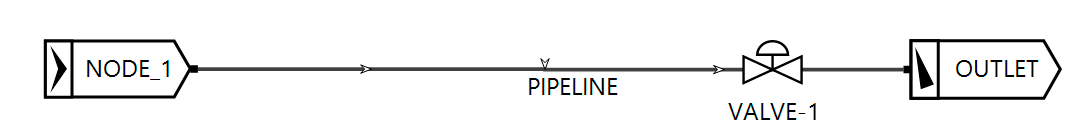
Figure 3: Pipeline physical model constructed in OLGA.

4 Comparative Analysis of Machine Learning Models for Slug Flow Prediction

Although physical models have the advantages of clear physics and high accuracy, their time-consuming computational simulation limits their application in rapid scheme screening and real-time control. Data-driven machine learning methods provide a new paradigm for solving this bottleneck. Its advantages lie in high computational efficiency and easy integration into existing control or monitoring systems.

There are various classic models in the field of machine learning. These models have significant differences in principle mechanisms, performance, and applicable scenarios. Their core advantages and disadvantages jointly determine the model selection logic in different scenarios. This paper adopts nine different machine learning models to predict slug flow in oil-gas-water three-phase flow.

4.1 Random Forest Model

Random Forest by employing Bootstrap resampling technique, this algorithm constructs K independent training subsets from the original multiphase flow dataset and trains K decision trees in parallel [32]. The specific mechanism of the model is illustrated in Fig. 4. During the prediction phase, the algorithm aggregates the outputs of all base classifiers (decision trees) and determines the final flow pattern category through a majority voting mechanism. This ensemble approach can effectively reduce the variance of a single high-bias model and enhance the robustness of slug flow identification in multiphase flow. Assuming that for an input operating condition vector x (containing features such as temperature, gas-liquid ratio, and water cut), For the input x , the prediction yielded by the k-th decision tree is denoted as h k x , the Random Forest’s final prediction Y ^ is shown in Eq. (1). Y^=argmaxc∈0,1∑k=1KIhkx=c(1) where: Y ^ denotes the final flow pattern prediction generated by the model; c is the flow pattern category label (taking values of 0 or 1); k denotes the decision tree’s index; K represents the total count of decision trees; h k x stands for the k-th decision tree’s independent prediction of the input feature vector x ; I ⋅ acts as an indicator function: it evaluates to 1 if the associated condition is met, and 0 in all other cases.

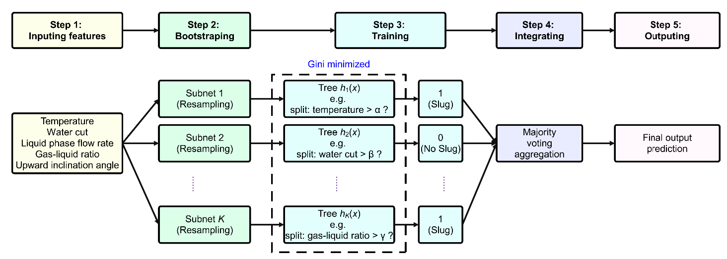
Figure 4: Random Forest model.

4.2 Decision Tree Model

The Decision Tree is constructed using the CART (Classification and Regression Tree) algorithm, and its essence is to recursively partition the high-dimensional feature space into non-overlapping rectangular regions [33]. At each non-leaf node, the algorithm iterates through all features and their split thresholds to find the optimal split point that maximizes the purity of the samples in the child nodes (i.e., minimizes the Gini impurity). Assuming that the current node contains a sample set D, the algorithm selects feature j and threshold t for splitting. Its objective function (split cost) J j , t is defined in Eq. (2), and the calculation formula for Gini impurity is shown in Eq. (3). Jj,t=mleftmGinileft+mrightmGiniright(2) GiniD=1−∑c=01pc(3) where: J j , t is the split cost of feature j at threshold t; m represents the overall sample count corresponding to the current node; m left/right correspond to the sample counts of the left-branched and right-branched child nodes generated after the splitting step, in sequence; G i n i left/right denote the Gini impurity metrics of the sample subsets associated with the left-branched and right-branched child nodes (resulting from the splitting process), correspondingly; p c is the proportion of samples belonging to category c (slug flow or non-slug flow) in the sample set.

4.3 XGBoost Model

As shown in Fig. 5, XGBoost (Extreme Gradient Boosting) is an additive model based on the Boosting strategy [34]. Different from the parallel computing of Random Forest, XGBoost adopts sequential iterative training. The goal of constructing the t-th tree f t x i is to fit the residual between the predicted value of the previous round of the model and the true flow pattern label. To prevent overfitting on high-noise pipeline data, XGBoost explicitly introduces a model complexity regularization term into the objective function and optimizes the gradient descent process using second-order Taylor expansion. The structured objective function L t for the t-th iteration is shown in Eq. (4), and the definition of the regularization term Ω f t is given in Eq. (5). Lt=∑i=1ngiftxi+12hift2xi+Ωft(4) Ωft=γT+12λ‖w‖2(5) where: i marks the identifier for each individual sample; n signifies the full size of the training sample set; g i and h i denote, in sequence, the first-order slope and second-order rate of change (of the loss function) relative to the forecast value from the prior iteration; f t x i stands for the additive forecast output of the t-th tree when handling sample i; T represents the count of terminal nodes; ‖ w ‖ 2 refers to the L2 measure associated with the weight vector of terminal nodes; γ is the punitive factor tied to the quantity of terminal nodes; λ denotes the L2 regularization factor applied to the weights of terminal nodes.

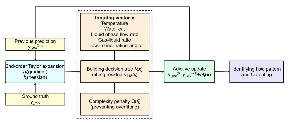
Figure 5: XGBoost model.

4.4 Naive Bayes Model

As shown in Fig. 6, the Naive Bayes approach draws on Bayes’ theorem within probabilistic analysis [35], and incorporates the strict premise of “conditional independence among features”. Given that pipeline operation data are all continuous variables, Gaussian Naive Bayes is adopted in this study. The model assumes that under a given flow pattern category c, each physical feature (such as liquid flow rate, water cut, gas-liquid ratio, etc.) follows a normal distribution, and the flow pattern is determined by maximizing the posterior probability. For a given operating condition vector x = x 1 , x 2 , … , x n , the flow pattern category prediction formula is shown in Eq. (6). Among them, the likelihood probability P x j | c follows a Gaussian distribution, as detailed in Eq. (7). y^=argmaxc∈0,1Pc∏j=1dPxj|c(6) Pxj|c=12πσj,c2exp−xj−μj,c22σj,c2(7) where: y ^ is the predicted category output by the model; P c is the prior probability of the category (derived from how often slug flow instances appear in the training dataset); j stands for the index corresponding to the feature dimension; d is the total dimension of the input feature vector; x j is the j-th feature variable in the input vector; P x j | c is the likelihood probability that feature j takes the value x j given the known flow pattern c; μ j , c and σ j , c 2 correspond to the average value and squared deviation of the j-th feature under category c, in that order.

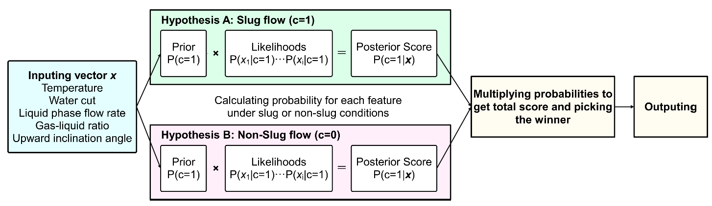
Figure 6: Naive Bayes model.

4.5 Logistic Regression Model

Logistic Regression constitutes a generalized linear framework employed to measure how each feature parameter contributes linearly to the likelihood of slug flow occurrence [36]. As shown in Fig. 7, the model performs linear weighting on the input feature vector x and maps it through the Sigmoid function to directly output the probability of slug flow occurrence under the current operating conditions. The prediction probability model is defined in Eq. (8). Among them, the model needs to optimize the weight parameters through maximum likelihood estimation (minimizing the logarithmic loss), as detailed in Eq. (9). Py=1|x=11+e−wTx+b(8) Jw,b=−1q∑i=1qyilogy^i+1−yilog1−y^i(9) where: P y = 1 | x is the predicted probability that the flow pattern label y is 1 (i.e., slug flow occurs) under the current operating condition x ; w is the weight coefficient vector, representing the influence degree of each physical parameter on the formation of slug flow in multiphase flow; w T is the transpose of the weight coefficient vector; b is the intercept term (bias); J w , b is the total loss function of the model; q is the total number of samples used for training; y i is the true label of the i-th sample (1 for slug flow, 0 for non-slug flow); y ^ i is the predicted probability that the model classifies the i-th sample as slug flow.

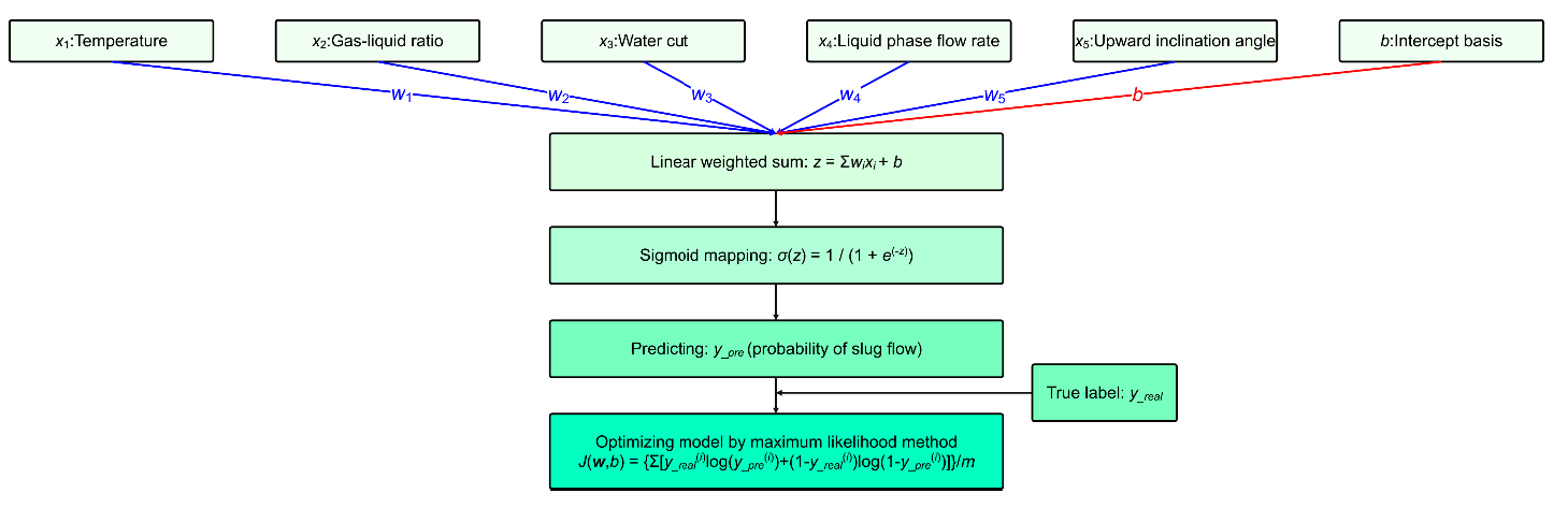
Figure 7: Logistic Regression model.

4.6 K-Means Model

K-Means is an unsupervised data grouping technique, and its core logic involves dividing a dataset into K distinct subsets through iterative tuning—strengthening the likeness of entries within one subset while weakening the likeness of entries across different subsets [37]. As shown in Fig. 8, it functions without labeled data, leaning solely on the inherent characteristics of sample attributes to complete the grouping process. This technique first sorts existing operating condition data into 2 subsets based on “whether slug flow has formed”, then works out the feature average (subset center) for each subset. When new pipeline operating condition data (such as temperature and water cut) is input, the technique gauges the separation between the new data and each subset center by applying the Euclidean distance calculation (as shown in Eq. (10)): L=∑(Xi−Ci)2(10) where: C i is the cluster center of the i-th category data; x i is the i-th sample vector.

If the separation between the newly input data and the subset center of a given group is narrower, it suggests that its attributes are more aligned with those of that group. The diagram below outlines the workflow of K-Means for slug flow forecasting.

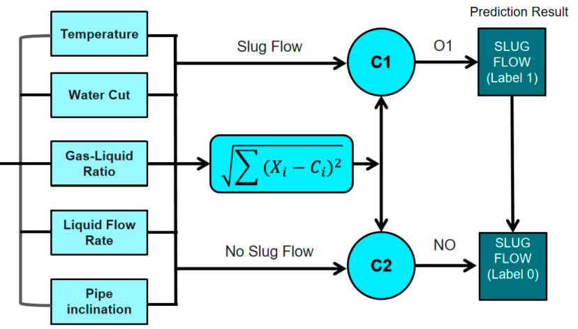
Figure 8: K-Means model.

4.7 Support Vector Machine Model

Support Vector Machine (SVM) is a classic binary classification algorithm in supervised learning [38]. It first uses the radial basis function kernel to address the non-linear correlation between slug flow features and formation results, mapping low-dimensional input features to a high-dimensional space. Then, it finds the hyperplane that maximizes the margin between “slug flow” and “non-slug flow” samples in the high-dimensional space. Finally, it determines whether the new operating condition features belong to the “slug flow” or “non-slug flow” category by judging which side of the hyperplane they are located in. This logic of “dimension elevation + maximum margin” not only adapts to the complex influence relationships of slug flow but also improves the stability of prediction.

Support Vector Machines (SVM) identify the ideal decision hyperplane by addressing a convex quadratic optimization task. Its target function is designed to expand the classification gap as much as possible, while permitting a limited level of classification errors, the target function is shown in Eq. (11): 12∥w∥2+C∑i=1nξi(11) where: w denotes the perpendicular vector corresponding to the decision hyperplane; b stands for the offset term associated with this decision hyperplane; C represents the punitive factor; ξ i refers to the extent to which a sample deviates from the expected boundary.

It is also required to satisfy ξ i ≥ 0 and the constraint, the constraint is shown in Eq. (12): yiwxi+b≥1−ξi(12) where: y i is the true label of the i-th sample, and x i is the feature vector of the i-th sample.

As depicted in Fig. 9, this diagram outlines the framework of an SVM-based slug flow forecasting model, and its process can be divided into three layers: First, the Input Layer receives 5 core characteristic parameters of the multiphase flow pipeline (temperature, water cut, gas-liquid ratio, liquid flow rate, and pipe inclination). After preprocessing via Feature Normalization, the data is fed into the SVM core optimization module. This component builds the ideal decision hyperplane by resolving a convex optimization task—composed of a target function paired with constraint terms. Finally, the Output Layer yields the binary classification result of “slug flow (Label 1)/non-slug flow (Label 0)”, enabling rapid identification of slug flow states in multiphase flow operating conditions.

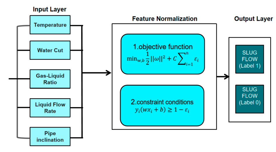
Figure 9: Support Vector Machine model.

4.8 BP Neural Network Model

The BP neural network constitutes a traditional multi-layer forward-passing network within supervised learning frameworks [39]. Its key function is to model the intricate nonlinear link between inputs and outputs via a repeated cycle: “calculating forecast values through forward signal transmission” and “adjusting weight parameters via backward error propagation”. It takes its name from the Back Propagation error-adjusting mechanism, and ranks among the foundational models for deep learning. MSE (Mean Squared Error) is a key parameter for evaluating the performance of neural network models, the calculation equation of MSE is shown in Eq. (13): MSE=1n∑i=1nyi−y^i2(13) where: M S E refers to the Mean Squared Error, n denotes the count of processing units in the neural network’s output stage, y i stands for the actual output of the i-th processing unit in this stage, and y ^ i is the forecasted output of that same i-th processing unit.

A standard BP-based network is typically composed of three stages: an input stage, a hidden stage, and an output stage. Each stage is fully linked to the others, with no internal connections within a single stage. The hidden stage may include several sub-stages; for most network architectures, a single hidden stage is adequate. Fig. 10 presents the framework diagram of a standard BP-based network.

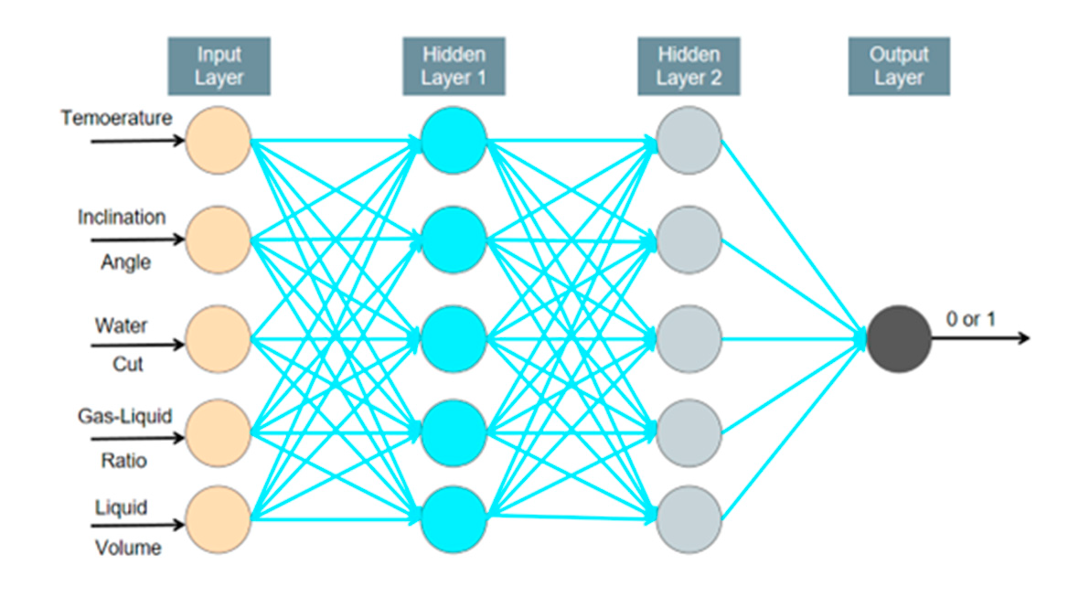
Figure 10: BP Neural Network model.

4.9 K-Nearest Neighbor Model

The principle of the K-Nearest Neighbors (KNN) model is based on the supervised learning logic of “category determined by sample similarity” [40]. Its core mechanism lies in the strong correlation between the slug flow state of the fluid and features such as temperature, water cut, liquid flow rate, and pipeline inclination angle—feature parameters of the same flow pattern (slug flow/non-slug flow) exhibit “local aggregation” in the high-dimensional space. Therefore, the KNN model first quantifies the feature difference between the new sample and the training samples through the L p distance equation. The L p distance equation is shown as Eq. (14): Lpxi,xj=∑l=1n|xil−xjl|p1p(14) where: L p x i , x j is the L p distance between two instance points x i and x j , p is the order of the L p distance, x i is the feature vector of the i-th instance point, x j is the feature vector of the j-th instance point, and n is the dimension of the feature vectors. x i l is the value of sample x i in the l-th feature dimension, x j l is the value of sample x j in the l-th feature dimension.

In the actual prediction of slug flow, the number of neighbors K is preset first. After obtaining the feature parameters from the input layer, the distances between the new sample and all samples in the training set are calculated using the Lp distance equation, and the K samples with the closest distances are selected (due to their high feature similarity, the flow pattern categories of these samples can better reflect the true state of the new sample). Then, based on the mechanism that “the flow pattern of the majority of samples represents the flow pattern of the new sample”, the voting decision module counts the category proportion of these K neighbors, and finally obtains the binary classification result of “slug flow/non-slug flow” at the output layer. As shown in Fig. 11 below, it illustrates the structural model diagram of the K-Nearest Neighbors (KNN) model.

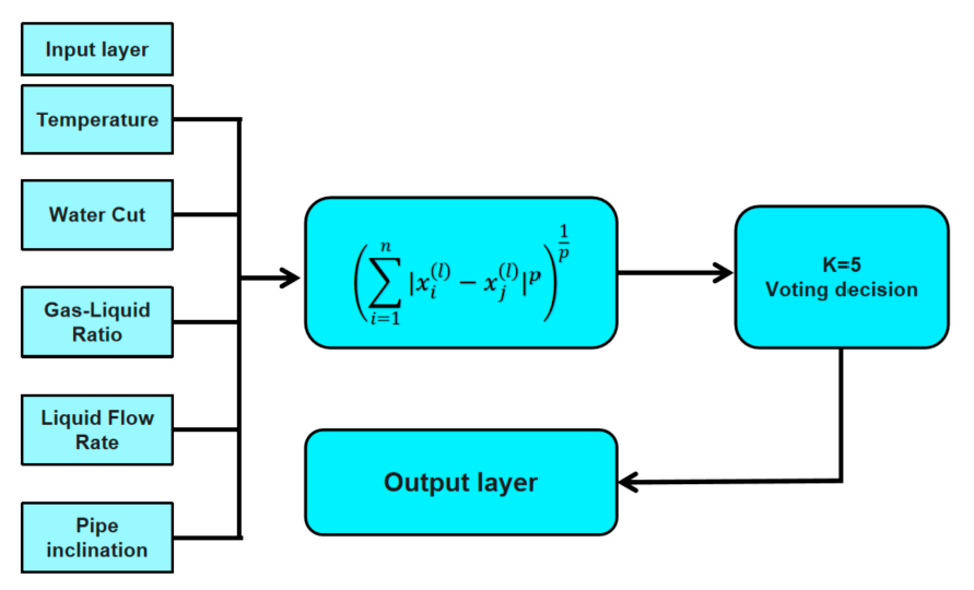
Figure 11: K-Nearest Neighbor model.

4.10 Model Evaluation Indicators

By and large, the strengths and limitations of distinct machine learning frameworks are mutually supplementary, while predictive precision stands as a critical metric to prioritize when choosing a model. Since different configurations of different machine learning models will affect the accuracy of model prediction, this paper to use the F1 function as an indicator to judge model accuracy. The F1 metric represents the harmonic average of Precision and Recall, requiring the prior calculation of both indicators. In slug flow prediction, high Precision indicates that the “slug flow alarm” triggered by the model is highly reliable, which can minimize unnecessary production interventions (thus reducing false positive costs); high Recall enables the model to capture the maximum number of actual slug flow events, guaranteeing the safety of the pipeline system (thereby cutting false negative costs). The formulation of the “F1 score priority” principle is specifically intended to strike an optimal balance between the two, with the goal of constructing a warning model that is both dependable and responsive. This metric selection criterion underscores the research’s focus on engineering practicality, which places equal emphasis on safety and efficiency.

Accuracy is defined as the proportion of cases predicted as “slug flow present” that are truly slug flow instances. High accuracy indicates that when an alarm is raised by the model, it is highly credible and warrants the attention of pipeline monitoring personnel. As shown in Eq. (15): Accuracy=TPTP+FP×100%(15) where: TP (True Positives) represents cases where slug flow actually occurs and is correctly predicted by the model, and FP (False Positives) denotes cases where slug flow does not occur but is incorrectly predicted by the model (false alarms).

Recall is characterized as the share of real-world “slug flow occurrence” instances that the model manages to detect correctly. This is considered one of the most critical indicators in slug flow prediction. High recall implies that genuinely hazardous slug flow conditions are rarely missed, which is essential for operational safety. As shown in Eq. (16): Recall=TPTP+FN×100%(16) where: FN (False Negatives) represents cases where slug flow actually occurs but is not predicted by the model (missed detections).

The F1 score is recognized as the optimal single metric for comprehensively evaluating model performance, as it identifies a balance when accuracy and recall are in conflict. As shown in Eq. (17):

When different models are compared, the priority of evaluation metrics is established as: F1 score greater than accuracy. That is, the model with the highest F1 score is prioritized. If the F1 scores are identical, accuracy is then compared. Should the accuracy also be equal, the model with the shorter training time is selected.

4.11 Hyperparameter Optimization and Validation Strategy

To guarantee the reproducibility and fairness of model comparison, a systematic hyperparameter optimization procedure was adopted. The optimization was carried out via Grid Search, with the objective function designed to maximize the F1 score. To strictly isolate tuning and testing processes, 5-fold Cross-Validation was executed solely on the 195 training samples. This ensures that the hyperparameters were adjusted without “accessing” the final test set (20%), thus avoiding data leakage. The specific implementation outcomes and the identified optimal parameters are elaborated in Section 5.1.

5 Case Study

5.1 Model Performance Comparison and Evaluation

To validate the universality of the established model, a typical undulating pipeline route is designed, as illustrated in Fig. 12. The total pipeline length is 15 km, with an inner diameter of 0.207 m. The pipe wall material is composite, with an absolute roughness of 5 × 10−5 m. The ambient temperature of the pipeline is set at 5°C, and the overall heat transfer coefficient is 0.6 W/(m2·°C). The simulation duration is configured for 3 days. Through the physical model, five key factors are analyzed: temperature (80°C, 120°C, 150°C), water cut (40%, 60%, 90%), liquid flow rate (100 t/d, 200 t/d, 300 t/d), gas-liquid ratio (3, 5, 15), and inclination angle of the uphill pipe segment (5°, 10°, 15°). A systematic cross-analysis of the five aforementioned factors yielded 243 simulated typical operating conditions.

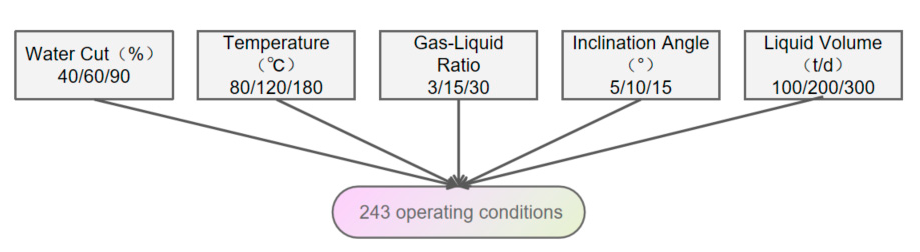
Figure 12: Slug flow cross operating conditions.

The oil-gas-water three-phase flow model simulates 243 operating conditions composed of varying temperatures, water cuts, gas-liquid ratios, liquid flow rates, and pipeline inclination angles. As shown in the following figure, it can be judged whether there is slug flow according to observations. When the inlet temperature is 120°C, the inlet flow rate is 2 kg/s, the gas-liquid ratio is 5 (since the data given in the engineering application is fixed, it is the ratio of the volume flow rate of gas in Nm3/d to the mass flow rate of liquid in t/d), the water cut is 90%, and the pipeline inclination angle is 5°, the simulation result is shown in Fig. 13. Depending on whether the slug length is 0, 243 sets of simulated conditions are labeled as “slug flow (1)” or “non-slug flow (0)” as training labels for the machine learning model. At the same time, five key influencing factors corresponding to each condition—temperature, water content, liquid flow rate, gas-liquid ratio, and pipe inclination—are used as input features for the machine learning model to complete the model training and testing.

Figure 13: Slug flow formation diagram in the pipeline under a certain operating condition.

The results of the single-variable analysis are summarized as follows:

• (1)With other main factors fixed, as the temperature rises from 40°C to 70°C, the number of slug flow occurrences increases from 42 to 53. The liquid phase viscosity decreases, making slug flow more likely to form.
• (2)With other main factors fixed, as the liquid phase flow rate decreases from 300 t/d to 100 t/d, the number of slug flow occurrences increases from 22 to 43. The liquid film at the bottom of the pipeline becomes thinner and less continuous, facilitating the formation of slug flow.
• (3)With other main factors fixed, as the water cut increases from 40% to 90%, the number of slug flow occurrences increases from 35 to 67. The liquid phase viscosity reduces, which is conducive to the formation of slug flow.
• (4)With other main factors fixed, as the gas-liquid ratio increases from 3 to 30, the number of slug flow occurrences increases from 17 to 72. The gas superficial velocity and gas kinetic energy increase, enhancing the gas’s ability to entrain and carry the liquid phase, thus making it easier to stir the liquid surface and form continuous slug segments.
• (5)With other main factors fixed, as the pipeline inclination angle increases from 5° to 15°, the number of slug flow occurrences increases from 44 to 55. The axial component of gravity promotes the accumulation of the liquid phase in low-lying or ascending sections, causing local blockages and triggering slug flow.

Before proceeding to the prediction tasks, the hyperparameters of the nine machine learning models were rigorously optimized based on the strategy described in Section 4.11. The specific search ranges and the finalized optimal parameters are summarized in Table 1. All computational experiments were conducted in a Python 3.9 environment using the Scikit-learn (v1.0.2) library.

The 243 sets of high-fidelity data generated by the simulations are utilized as the training and testing database for machine learning. They are randomly divided into a training set (195 sets) and a testing set (48 sets) at an approximate ratio of 4:1. The nine machine learning models mentioned in the previous chapter are employed for slug flow prediction. The F1 scores and accuracy rates obtained for each model are shown in Fig. 14. Based on the comparative results, Decision Tree, Random Forest, XGBoost, Logistic Regression, and Naïve Bayes all achieve both an F1 score and accuracy of 100%, indicating excellent predictive performance by these five models.

In sharp contrast, the unsupervised K-Means algorithm (serving as a baseline) yielded the lowest accuracy of 62.96%. This significant performance gap empirically verifies that the slug flow data does not form distinct, compact clusters in the Euclidean space. Instead, the classification boundaries are highly non-linear and overlapping, thereby highlighting the necessity of employing supervised learning models (such as BP NN and XGBoost) to capture these complex mapping relationships.

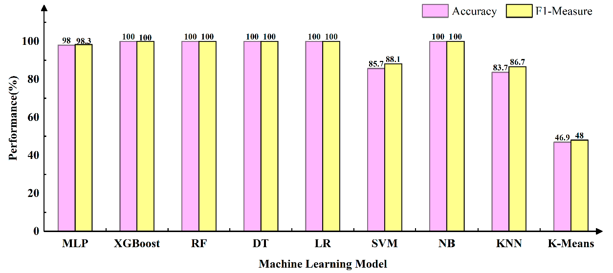
Figure 14: Comparison of evaluation metrics for different machine learning models.

To test the model’s predictive capability for unknown, non-preset operating conditions, the research randomly generated 108 new sets of operating conditions within the continuous value ranges of the aforementioned factors (e.g., temperature 80–150°C). The parameter combinations of these new conditions did not appear in the previous training set, thus constituting an independent test set that more closely resembles the continuously varying scenarios of actual operation., 108 sets of new operating conditions outside the physical model database are randomly generated for prediction, with temperature ranging from 80–150°C, water cut from 40%–90%, liquid flow rate from 100 t/d–300 t/d, gas-liquid ratio from 3–15, and pipeline inclination angle from 5°–15°. The prediction results are compared with the detailed simulation results of the physical model. As shown in Fig. 15, the XGBoost and BP neural network models achieve the highest prediction accuracy, up to 95%. This indicates that these two models are reliable and can be used for the rapid and accurate identification of slug flow under different operating conditions.

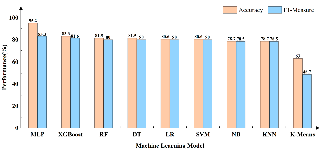
Figure 15: Different machine learning prediction models.

5.2 Feature Importance Analysis and Mechanistic Verification

To quantitatively validate the influence of operating parameters on slug flow formation, feature importance scores were extracted from the optimized ensemble learning models (Random Forest and XGBoost). As shown in Fig. 16, the data-driven analysis provides a comprehensive ranking of the five factors:

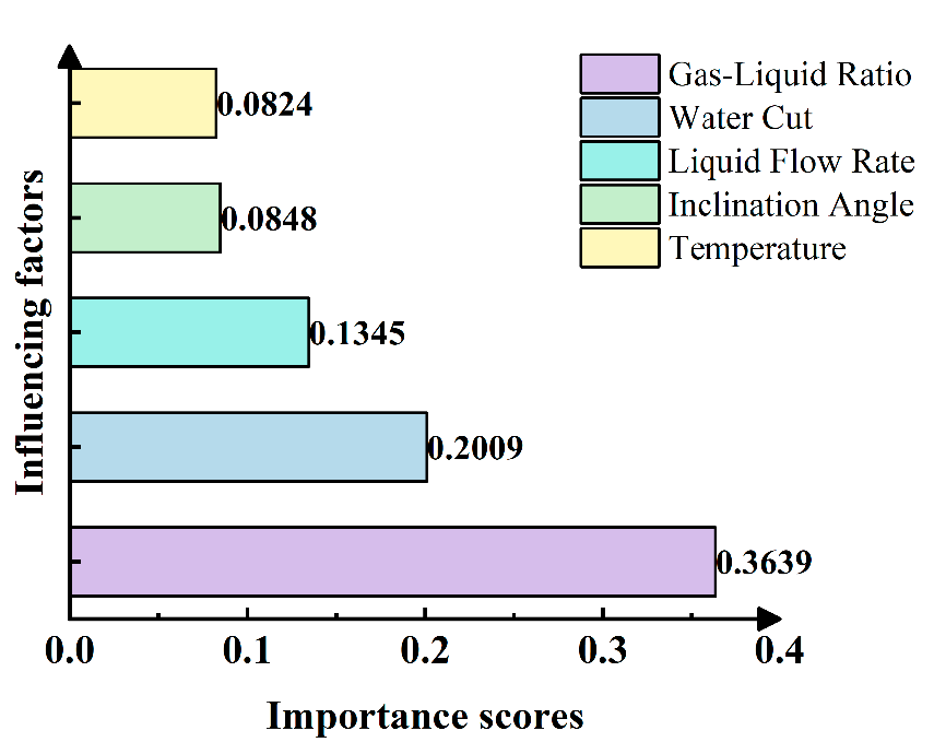
Figure 16: Normalized feature importance ranking of the five operating parameters derived from the optimized ensemble learning models.

• (1)Gas-Liquid Ratio (GLR) is identified as the most critical factor (Score: 0.364). This confirms that the gas phase kinetic energy is the primary driver for interfacial shear stress. A higher GLR intensifies the Kelvin-Helmholtz instability, serving as the direct hydrodynamic trigger for liquid film instability and slug initiation.
• (2)Water Cut ranks second (Score: 0.201). As analyzed in Section 2, the variation in water cut significantly alters the mixture’s effective viscosity and density. An increase in viscosity enhances the stability of the liquid film, thereby modulating the wave growth rate and the flow pattern transition threshold.
• (3)Liquid Flow Rate ranks third (Score: 0.135). Physically, the superficial liquid velocity determines the basic liquid holdup in the pipeline. A sufficient liquid volume is the structural prerequisite for the liquid film to bridge the pipe cross-section, forming the body of stable liquid slugs.
• (4)Inclination Angle ranks fourth (Score: 0.085). The pipe inclination determines the gravitational component acting along the flow direction. This force directly influences the liquid accumulation and drainage rates at the pipe bottom, acting as a crucial boundary condition that shifts the transition boundaries between stratified and slug flow.
• (5)Temperature ranks fifth (Score: 0.082). While its direct weight is lower, it functions by altering fluid physical properties (PVT behavior). Variations in temperature affect gas density and liquid viscosity, which indirectly modify the friction factors and phase distribution, serving as a thermodynamic constraint on the flow system.

In summary, the ML model’s statistical ranking aligns perfectly with the sensitivity trends observed in the simulation experiments (in Section 5.1), verifying that the model has successfully captured the underlying flow assurance mechanisms.

5.3 Generalization Capability Analysis and Overfitting Discussion

A significant performance divergence was observed between the internal test set (Fig. 14) and the new external operating conditions (Fig. 15). While models like Decision Tree achieved perfect scores (100%) on the initial 48-sample test split, their performance degraded significantly on the 108 new conditions.

This discrepancy highlights a critical mechanism of overfitting to the grid-based data structure. Since the training dataset was generated using discrete grid sampling (e.g., fixed temperatures of 80°C, 120°C, 150°C), the Decision Tree constructed rigid, step-like decision boundaries that effectively “memorized” these specific grid points. Consequently, it achieved perfect scores on the initial test split—which followed the same grid distribution—but failed to generalize when predicting continuous, off-grid values (e.g., 105°C) in the external dataset.

In contrast, XGBoost and BP Neural Network maintained high accuracy (95.2%, 83.3%) on the external dataset, demonstrating superior generalization. This robustness is attributed to their advanced regularization mechanisms that enforce smoother decision boundaries:

• (1)XGBoost: It employs a regularized objective function that explicitly includes a complexity penalty term. This prevents the model from fitting high-frequency variations or steps between grid points.
• (2)BP Neural Network: By learning global non-linear mapping relationships through distributed weights, it captures the continuous trend of physical laws rather than isolating local rules.

Thus, despite the “perfect” internal scores of simpler models, XGBoost and BP NN are confirmed as the most reliable tools for practical engineering applications where operating conditions vary continuously.

6 Conclusion

This study conducts a systematic analysis of how slug flow develops in oil-gas-water multiphase pipelines, and constructs a forecasting framework built on a BP-based network. Through inquiry and evaluation, the key findings outlined below are summarized:

• (1)Factors including elevated temperature, higher water cut, lower liquid flow rate, larger gas-liquid ratio, and risen upward pipeline inclination are all found to significantly enhance flow instability, thereby promoting the formation of slug flow.
• (2)Through a comparison of the forecasting outcomes of nine machine learning frameworks, it is found that Decision Tree, Random Forest, XGBoost, Logistic Regression, and Naive Bayes all reach an F1 score and precision of 100%—this shows that these models perform exceptionally well in forecasting on the test dataset.
• (3)When 108 entirely new operating conditions outside the original physical model database are randomly generated for prediction and compared against detailed physical simulations, the BP Neural Network models are identified as achieving the highest prediction accuracy, reaching 95%.
• (4)A critical evaluation of model generalization reveals that although simple models (e.g., Decision Tree) achieved perfect scores on the internal test set, this was a result of memorizing the discrete training grid, leading to poor performance on continuous external datasets. Conversely, XGBoost and BP Neural Network demonstrated superior robustness (95.2%, 83.3%). Their inherent regularization mechanisms successfully prevented overfitting, enabling them to capture the underlying continuous physical laws of slug flow formation.

In summary, this research not only deepens the understanding of slug flow formation mechanisms but also provides a complete technical pathway from high-fidelity simulation to rapid prediction. This holds significant theoretical importance and practical engineering value for ensuring the safe, stable, and efficient operation of oil and gas gathering and transportation pipelines. To further refine this pathway for complex real-world environments, a hybrid field-correction strategy is proposed for future implementation. By utilizing high-quality field measurements to calibrate the pre-trained models, systematic simulator-induced biases can be effectively rectified. This evolution from “simulation-driven” to “field-calibrated” intelligence will ensure the highest reliability for future engineering deployments.

References

1. Arabi A , Stiriba Y , Pallares J . Physically-based models for predicting the bubbly-to-slug flow transition in vertical downward gas–liquid two-phase flow. Int J Multiphase Flow. 2026; 197: 105610. doi:10.1016/j.ijmultiphaseflow.2026.105610. [Google Scholar] [CrossRef]
2. Rezavand M , Hu X . Numerical simulation of two-phase slug flows in horizontal pipelines: A 3-D smoothed particle hydrodynamics application. Eur J Mech B-Fluid. 2024; 104: 56– 67. doi:10.1016/j.euromechflu.2023.11.005. [Google Scholar] [CrossRef]
3. Padrino JC , Srinil N , Kurushina V , Swailes D . Prediction of unsteady slug flow in a long curved inclined riser with a slug tracking model. Int J Multiphase Flow. 2023; 162: 104410. doi:10.1016/j.ijmultiphaseflow.2023.104410. [Google Scholar] [CrossRef]
4. Taitel Y , Dukler AE . A model for slug frequency during gas-liquid flow in horizontal and near horizontal pipes. Int J Multiphase Flow. 1977; 3( 6): 585– 96. doi:10.1016/0301-9322(77)90031-3. [Google Scholar] [CrossRef]
5. Davies SR . Studies of two-phase intermittent flow in pipelines [ dissertation]. London, UK: University of London; 1992. [Google Scholar]
6. Barnea D , Taitel Y . A model for slug length distribution in gas-liquid slug flow. Int J Multiphase Flow. 1993; 19( 5): 829– 38. doi:10.1016/0301-9322(93)90046-W. [Google Scholar] [CrossRef]
7. Ma L , Li W , Wang Y , Zhang P , Wang L , Liu X . Numerical simulation of gas-liquid flow in a horizontal elbow. Fluid Dyn Mater Process. 2025; 21( 1): 107– 19. doi:10.32604/fdmp.2024.058295. [Google Scholar] [CrossRef]
8. Li S , Wang J , Ma T , Deng G , Li W . Characterization of purged gas-liquid two-phase flow in a molten salt regulating valve. Fluid Dyn Mater Process. 2025; 21( 4): 959– 88. doi:10.32604/fdmp.2025.059570. [Google Scholar] [CrossRef]
9. Lyu L . Theoretical model of gas-liquid severe slugging in pipeline-riser systems. Oil Gas Storage Transp. 2018; 37( 10): 1095– 100. (In Chinese). [Google Scholar]
10. Dang T , Qi H , Zhang P . Advances in gas-liquid two-phase serious slug flow in vertical pipes. Yunnan Chem Technol. 2019; 46( 2): 46– 8. (In Chinese). [Google Scholar]
11. Ren J , Shao C , Wang J , Wang Z , Gao X , Zhang Z , et al. Two-phase flow characteristics of gas-liquid flow in horizontal flow experimental research. China Meas Test. 2025; 51( Suppl 1): 99– 104. (In Chinese). [Google Scholar]
12. Wang J , Jia Z , Niu G . Study of the flow patterns propagation behavior of oil-gas two-phase flow in the large diameter pipes. J Eng Thermophys. 2005; 26( Suppl 1): 137– 9. (In Chinese). [Google Scholar]
13. Gonçalves JL , Mazza RA . A transient analysis of slug flow in a horizontal pipe using slug tracking model: Void and pressure wave. Int J Multiphase Flow. 2022; 149: 103972. doi:10.1016/j.ijmultiphaseflow.2022.103972. [Google Scholar] [CrossRef]
14. Gonçalves JL , Mazza RA . Slug flow parameters applied to dynamic riser analysis. Int J Multiphase Flow. 2024; 171: 104670. doi:10.1016/j.ijmultiphaseflow.2023.104670. [Google Scholar] [CrossRef]
15. Nydal OJ , Banerjee S . Dynamic slug tracking simulations for gas-liquid flow in pipelines. Chem Eng Commun. 1996; 141( 1): 13– 39. doi:10.1080/00986449608936408. [Google Scholar] [CrossRef]
16. Al-Safran EM , Sarica C , Zhang HQ , Brill JP . Probabilistic/mechanistic modeling of slug-length distribution in a horizontal pipeline. SPE Prod Facil. 2005; 20( 2): 160– 72. doi:10.2118/84230-PA. [Google Scholar] [CrossRef]
17. Rosa ES , Mazza RA , Morales RE , Rodrigues HT , Cozin C . Analysis of slug tracking model for gas–liquid flows in a pipe. J Braz Soc Mech Sci Eng. 2015; 37( 6): 1665– 86. doi:10.1007/s40430-015-0331-7. [Google Scholar] [CrossRef]
18. Grigoleto MM , Bassani CL , Conte MG , Cozin C , Barbuto FAA , Morales REM . Heat transfer modeling of non-boiling gas-liquid slug flow using a slug tracking approach. Int J Heat Mass Transf. 2021; 165: 120664. doi:10.1016/j.ijheatmasstransfer.2020.120664. [Google Scholar] [CrossRef]
19. Guo C , Zhang H , Qian Z , Liu M . Smoothed-interface SPH model for multiphase fluid-structure interaction. J Comput Phys. 2024; 518: 113336. doi:10.1016/j.jcp.2024.113336. [Google Scholar] [CrossRef]
20. Guo C , Zhang H , Sun S , Qian Z , Liu M . A hybrid compressible-incompressible SPH model with adaptive iteration and GPU-optimization for multiphase flows. J Comput Phys. 2025; 546: 114513. doi:10.1016/j.jcp.2025.114513. [Google Scholar] [CrossRef]
21. Diehl FC , Gerevini GG , Machado TO , Quelhas AD , Anzai TK , Bitarelli T , et al. Anti-slug control design: Combining first principle modeling with a data-driven approach to obtain an easy-to-fit model-based control. J Pet Sci Eng. 2021; 207: 109096. doi:10.1016/j.petrol.2021.109096. [Google Scholar] [CrossRef]
22. Yin PB , Zhang P , Cao XW , Li X , Li YH , Bian J . Effect of SDBS surfactant on gas–liquid flow pattern and pressure drop in upward-inclined pipelines. Exp Therm Fluid Sci. 2022; 130: 110507. doi:10.1016/j.expthermflusci.2021.110507. [Google Scholar] [CrossRef]
23. Zhang P , Cao X , Peng F , Xu Y , Guo D , Li X , et al. High-accuracy recognition of gas–liquid two-phase flow patterns: A Flow–Hilbert–CNN hybrid model. Geoenergy Sci Eng. 2023; 230: 212206. doi:10.1016/j.geoen.2023.212206. [Google Scholar] [CrossRef]
24. Cao X , Yang K , Wang H , Bian J . Gas–liquid–hydrate flow characteristics in vertical pipe considering bubble and particle coalescence and breakage. Chem Eng Sci. 2022; 252: 117249. doi:10.1016/j.ces.2021.117249. [Google Scholar] [CrossRef]
25. Açıkgöz M , França F , Lahey RT . An experimental study of three-phase flow regimes. Int J Multiphase Flow. 1992; 18( 3): 327– 36. doi:10.1016/0301-9322(92)90020-H. [Google Scholar] [CrossRef]
26. Wegmann A , Melke J , Rudolf von Rohr P . Three phase liquid-liquid-gas flows in 5.6 mm and 7 mm inner diameter pipes. Int J Multiphase Flow. 2007; 33( 5): 484– 97. doi:10.1016/j.ijmultiphaseflow.2006.10.004. [Google Scholar] [CrossRef]
27. Bendiksen KH , Malnes D , Moe R , Nuland S . The dynamic two-fluid model OLGA: Theory and application. SPE Prod Eng. 1991; 6( 2): 171– 80. doi:10.2118/19451-PA. [Google Scholar] [CrossRef]
28. Raimondi L . Compositional simulation of two-phase flows for pipeline depressurization. SPE J. 2017; 22( 4): 1242– 53. doi:10.2118/185169-PA. [Google Scholar] [CrossRef]
29. Sur A , Liu D . Adiabatic air-water two-phase flow in circular microchannels. Int J Therm Sci. 2012; 53: 18– 34. doi:10.1016/j.ijthermalsci.2011.09.021. [Google Scholar] [CrossRef]
30. Beggs HD , Brill JP . A study of two-phase flow in inclined pipes. J Pet Technol. 1973; 25( 5): 607– 17. doi:10.2118/4007-PA. [Google Scholar] [CrossRef]
31. Sakaguchi H . Coupled modified Baker’s transformations for the Ising model. Phys Rev E. 1999; 60( 6): 7584– 7. doi:10.1103/PhysRevE.60.7584. [Google Scholar] [CrossRef]
32. Sun G , Wang J , Cai W , Shi L , Yao B , Yang F . A blending model for predicting flow rate of crude oil pipeline by integrating Leapienzon friction formula with random forest algorithm. Flow Meas Instrum. 2025; 106: 102971. (In Chinese). doi:10.1016/j.flowmeasinst.2025.102971. [Google Scholar] [CrossRef]
33. Charbuty B , Abdulazeez AM . Classification based on decision tree algorithm for machine learning. J Appl Sci Technol Trends. 2021; 2( 1): 20– 8. doi:10.38094/jastt20165. [Google Scholar] [CrossRef]
34. Kong L , Suganthan PN , Snášel V , Ojha V , Pan JS . Enhancing sampling performance in XGBoost by ensemble feature engineering. Pattern Recognit. 2026; 176: 113169. doi:10.1016/j.patcog.2026.113169. [Google Scholar] [CrossRef]
35. Kovács EA , Ország A , Pfeifer D , Benczúr A . Generalized Naive Bayes. Pattern Recognit. 2026; 174: 112927. doi:10.1016/j.patcog.2025.112927. [Google Scholar] [CrossRef]
36. Consolo A , Manno A , Amaldi E . Binary kernel logistic regression: A sparsity-inducing formulation and a convergent decomposition training algorithm. Comput Oper Res. 2026; 188: 107363. doi:10.1016/j.cor.2025.107363. [Google Scholar] [CrossRef]
37. Kim J , Lim J . Strong consistency of sparse K-means clustering. J Stat Plan Inference. 2026: 106408. doi:10.1016/j.jspi.2026.106408. [Google Scholar] [CrossRef]
38. Dalir R , Amiri A , Alamdar F , Kaya A . Online semi-supervised independent support vector machines. Int J Approx Reason. 2026: 109658. doi:10.1016/j.ijar.2026.109658. [Google Scholar] [CrossRef]
39. Mei C , Chen H , Zhu J , Chen X , Zhang C , Jiang H . Enhancing performance of detecting AFB1 in wheat via electronic nose combined with back-propagation neural network. Microchem J. 2025; 215: 114189. doi:10.1016/j.microc.2025.114189. [Google Scholar] [CrossRef]
40. Guessoum D , Takruri M , Rabih M , Farhat M , Badawi SA . K-Nearest Neighbors hybrid method for maximum power point tracking under partial shading for photovoltaic power systems. Results Eng. 2025; 27: 106694. doi:10.1016/j.rineng.2025.106694. [Google Scholar] [CrossRef]
Cite This Article
Copyright © 2026 The Author(s). Published by Tech Science Press.
This work is licensed under a Creative Commons Attribution 4.0 International License , which permits unrestricted use, distribution, and reproduction in any medium, provided the original work is properly cited.
Downloads
Citation Tools