
 Login
Login Register
 Submit a Paper
 Propose a Special lssue
 Open Access
ARTICLE
A Unified Semi-Empirical Model for Low-Velocity Corrosion Mitigation and High-Velocity Erosion Enhancement in CO2-Containing Environments
1 Sinopec Natural Gas Branch, Beijing, China
2 Natural Gas Yuji Pipeline Branch, Jinan, China
3 School of Petrochemical Technology, Lanzhou University of Technology, Lanzhou, China
* Corresponding Authors: Xingda Tong. Email: ; Zhihui Wang. Email:
(This article belongs to the Special Issue: Theoretical Foundations and Applications of Multiphase Flow in Pipeline Engineering)
Fluid Dynamics & Materials Processing 2026, 22(9), 4 https://doi.org/10.32604/fdmp.2026.087557
Received 29 June 2026; Accepted 08 September 2026; Issue published 28 September 2026
 View Full Text
 Download PDF
Abstract
This study develops a unified, material-specific semi-empirical framework to describe both low-velocity corrosion mitigation and high-velocity erosion-corrosion enhancement in CO2-containing environments. L360, 20# and X65 steels were investigated using static weight-loss and electrochemical tests, together with dynamic erosion-corrosion experiments and SEM/EDS characterization. Static tests were conducted at total pressures of 3–7 MPa, CO2 partial pressures of 4–60 kPa, and temperatures of 10–60°C, while dynamic tests were performed at 3.5 MPa total pressure, 40 kPa CO2 partial pressure, and 25°C, over velocities of 0–50 m/s and impingement angles of 0–80°. Static corrosion rates increased with increasing CO2 partial pressure and temperature. Under dynamic conditions, corrosion rates initially decreased with velocity, indicating a low-velocity mitigation effect, before increasing at higher velocities as erosion became increasingly influential, with the maximum measured rate occurring at an impingement angle of 45°. Because SEM/EDS evidence did not establish the presence of a crystalline FeCO3-dominated protective film, the low-velocity behavior was represented phenomenologically through a surface-coverage/deposit effect rather than attributed to a specific scale-growth mechanism. The resulting model combines a de Waard-type static corrosion baseline with exponential coverage-induced mitigation, a critical-velocity erosion enhancement term, and a modified Finnie angular function. Applied to the present dataset, the framework achieved an R2 of 0.9308 and a Root Mean Square Error (RMSE) of 0.0319.Keywords
Internal CO2 corrosion is one of the most common forms of metallic degradation in wet-gas gathering pipelines, gas-field produced-water systems, and oil and gas surface gathering systems. When free water wets the pipe wall, CO2 dissolves into the aqueous phase and participates in carbonate equilibria, forming H2CO3, HCO3−, and CO32− species. Carbon-steel corrosion is consequently driven by coupled cathodic reduction reactions and anodic iron dissolution [1]. The CO2 corrosion rate is therefore jointly controlled by temperature, CO2 partial pressure, pH, ionic composition, Fe2+ concentration, and hydrodynamic conditions. Temperature and CO2 partial pressure determine the reaction kinetics and the degree of solution acidification, pH directly affects cathodic reactions and corrosion-product precipitation, and flow velocity and wall shear stress alter the mass-transfer boundary layer, corrosion-product film stability, and erosion-damage intensity [2].
A variety of empirical, semi-empirical and mechanistic models have been developed for engineering prediction of CO2 corrosion. The de Waard-Milliams model relates corrosion rate to temperature and CO2 partial pressure [3], while the DW95 formulation introduces reaction- and mass-transfer-controlled resistances to account for flow effects [4]. The NORSOK M-506 model incorporates temperature, CO2 partial pressure, pH and wall shear stress [5], and the CORPOS framework extends engineering risk assessment to pipeline systems with internal liquids [6]. Mechanistic models further describe electrochemical reactions, species transport and FeCO3 precipitation or film growth [7,8]. For flowing systems, the Tulsa model couples corrosion, mass transfer and sand-related erosion effects [9], whereas the Ohio model addresses sweet corrosion in horizontal multiphase flow [10]. Additional engineering prediction approaches for oil and gas pipelines have been reported in Refs. [11,12]. Li et al. [13] evaluated corrosion models for CO2-flooding production and transportation components, Remita et al. [14] simplified species-transport calculations in the diffusion boundary layer, and Gong et al. [15] developed a generalized prediction method for natural-gas pipeline steels.
Although these models provide an important basis for CO2 corrosion prediction, limitations remain when flow corrosion and erosion-corrosion occur simultaneously. Conventional velocity terms generally emphasize flow-enhanced mass transfer and therefore tend to predict a monotonic increase in corrosion rate with increasing flow velocity. In actual flowing CO2 corrosion, however, flow can promote both reactant transport and the formation or removal of surface corrosion products. When the blocking effect of surface coverage exceeds the enhancement of mass transfer, the corrosion rate may become lower than that under static conditions. Once the flow velocity further increases and exceeds the stability threshold of the surface layer, erosion-induced damage can expose fresh metal and cause the corrosion rate to increase again [16].
Choi et al. [17] and Jiang et al. [18] reported that loose, low-density FeCO3 deposits may form on carbon-steel surfaces at low temperature. Such deposits are generally weakly adherent and provide limited isolation of the substrate from the corrosive medium. Their presence is therefore not equivalent to formation of a dense protective FeCO3 film. Film nucleation, growth and protectiveness depend on local supersaturation, pH, temperature, Fe2+ concentration, steel microstructure and flow-induced shear [19,20]. When phase identity and layer continuity are not established experimentally, the influence of corrosion products is more appropriately represented as a generalized surface-coverage effect than as explicit FeCO3 film-growth kinetics.
Computational fluid dynamics (CFD) and machine learning are increasingly being applied to corrosion prediction under complex geometries and large-data conditions. Owen et al. [21] coupled CFD-derived local mass-transfer coefficients with empirical CO2 corrosion relationships to predict corrosion in a sudden-expansion pipe geometry. Thorat et al. [22] further developed a CFD-driven mass-transfer model to calculate viscous sublayer thickness and turbulent diffusion parameters. Machine-learning models can improve the fitting efficiency for complex multivariable relationships; however, they typically require large datasets and still require mechanistic constraints to ensure reliable small-sample extrapolation and physical interpretability [23,24,25]. Therefore, for studies with limited experimental data but a need to retain physical interpretability, a semi-empirical coupled model remains practically meaningful.
In this study, L360, 20#, and X65 pipeline steels were selected as the target materials. Static weight-loss and electrochemical tests were first used to determine the effects of temperature, CO2 partial pressure, and pH on the corrosion process. Dynamic erosion-corrosion tests were then used to reveal the effects of flow velocity and impingement angle on corrosion rate. Finally, based on a de Waard-type static model, relevant influence terms were introduced to establish material-specific flow-erosion coupled corrosion models for the three steels.
The experimental materials were L360, X65, and 20# alloy pipeline steels obtained from qualified pipelines in an oil and gas field. Their chemical compositions are listed in Table 1. The three steels are commonly used pipeline materials in oil and gas transportation systems and represent different strength grades.
Table 1: Chemical compositions of L360, X65, and 20# steels.
| Material | Element | C | Si | Mn | P | S | Cr | Ni | Cu | Mo | Fe |
|---|---|---|---|---|---|---|---|---|---|---|---|
| L360 | [wt%] | 0.13 | 0.24 | 1.12 | 0.012 | 0.003 | 0.07 | 0.01 | 0.06 | 0.02 | bal |
| 20# | [wt%] | 0.21 | 0.25 | 0.6 | 0.014 | 0.0028 | 0.034 | 0.02 | 0.002 | — | bal |
| X65 | [wt%] | 0.075 | 0.235 | 1.45 | 0.012 | 0.002 | 0.064 | 0.076 | 0.026 | 0.145 | bal |
The test solution contained 5 g/L NaCl, equivalent to 5000 mg/L as NaCl. Because site-specific water-chemistry and sand-loading data were unavailable, the solution and solid-phase conditions were defined as controlled laboratory parameters rather than as an exact reproduction of a single field location.
2.2.1 High-Pressure Weight-Loss Tests
The weight-loss method was used to determine the average corrosion rates of the metallic materials under different corrosive environments. Steel pipes with the same compositions as the target pipelines were machined into standard coupons. Two coupon geometries were used: conventional corrosion-rate coupons (40 × 13 × 2 mm) and coupons for detailed corrosion-morphology analysis (10 × 10 × 10 mm). Before testing, all coupons were degreased with acetone, cleaned with absolute ethanol, dried with cold air, and weighed using an electronic balance with an accuracy of 0.1 mg. The coupons were subsequently mounted in the high-temperature and high-pressure autoclave shown in Fig. 1 using a specially designed insulated bolt fixture to ensure electrical insulation from the autoclave body.
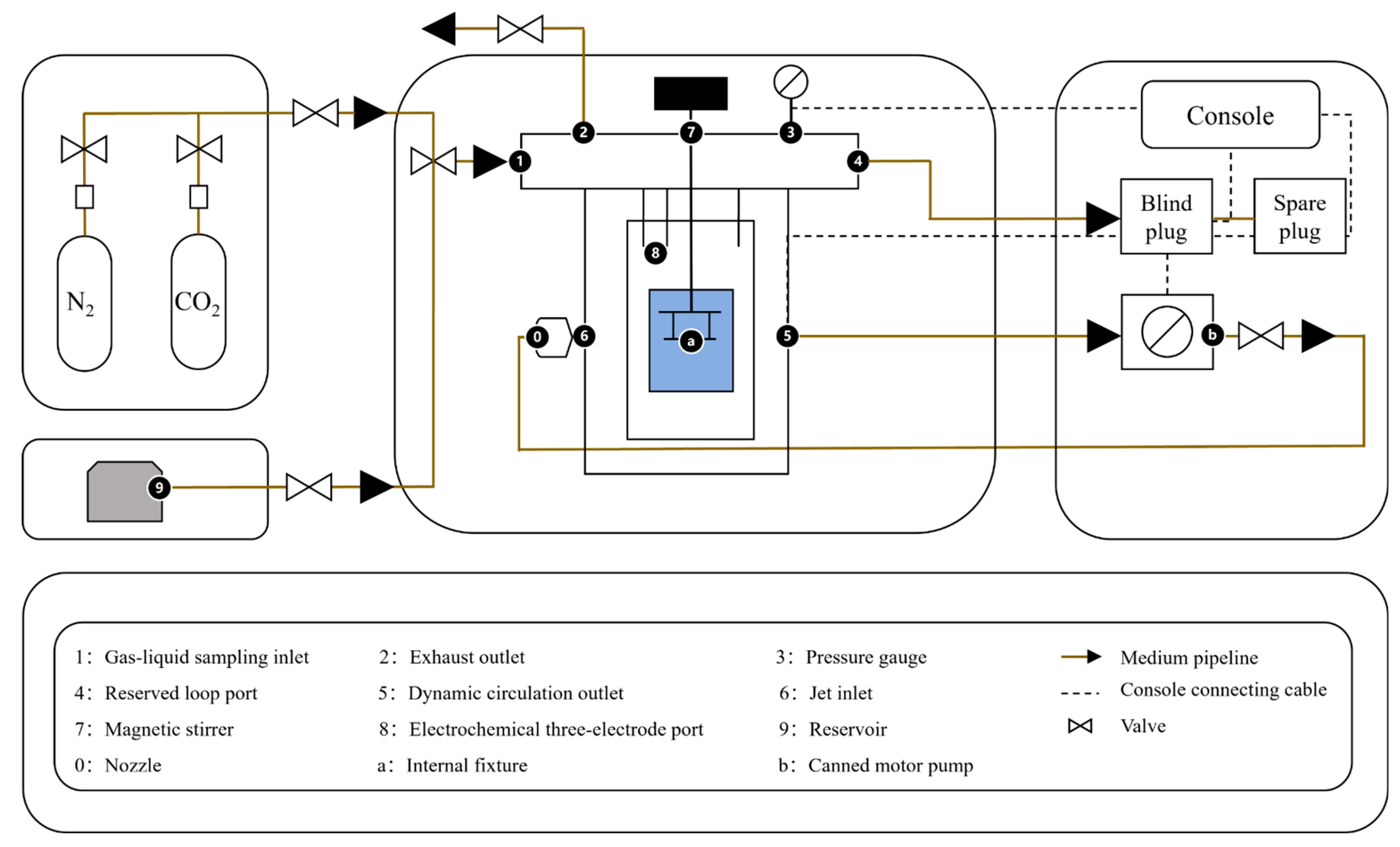
Figure 1: High-temperature and high-pressure corrosion test apparatus.
After the autoclave was sealed, N2 was introduced into the solution for more than 2 h to remove dissolved oxygen, followed by CO2 purging for more than 4 h to achieve saturation. The static test matrices were material-specific: L360 was tested at 3.5 MPa, CO2 partial pressures of 20–60 kPa and temperatures of 10–60°C; 20# steel at 3 MPa, 10–30 kPa and 10–50°C; and X65 steel at 7 MPa, 10–40 kPa and 20–60°C. After the prescribed temperature and pressure stabilized, the coupons were immersed for 72 h. The exposed coupons were rinsed with deionized water, and corrosion products were removed ultrasonically for 3 min in a solution containing 500 mL hydrochloric acid and 3.5 g hexamethylenetetramine diluted to 1 L with deionized water. The coupons were then dried with cold air, reweighed, and evaluated using Eq. (1):
The mass-loss flux from Eq. (1) was converted to corrosion penetration rate using specimen density and unit conversion; all corrosion-rate values in Table 2 and Table 3, figures and model equations are reported consistently as mm/a.
2.2.2 High-Pressure Electrochemical Tests
Before each electrochemical test, the simulated accumulated liquid corresponding to the target condition was deaerated with high-purity N2 (99.99%) for more than 2 h, as shown in Fig. 1, and then saturated with CO2 for more than 4 h before sealing. Electrochemical measurements were performed using a CS2350M dual-potentiostat electrochemical workstation in a three-electrode configuration. A large-area platinum sheet was used as the counter electrode, and a high-temperature and high-pressure Ag/AgCl electrode was used as the reference electrode. The working electrodes were prepared from the corresponding qualified pipeline steels. The electrode specimens were 10 × 10 × 8 mm, and the exposed area after assembly in the customized high-pressure working-electrode holder was 1 cm2. Before testing, the working electrodes were sequentially ground with metallographic abrasive papers from 80# to 2000#, rinsed with deionized water, wiped with absolute ethanol, and dried with cold air. The open-circuit potential (OCP) was monitored before electrochemical measurements. After the OCP stabilized, electrochemical impedance spectroscopy (EIS) and potentiodynamic polarization tests were performed. The EIS frequency range was 10−2–105 Hz, and the perturbation amplitude was 10 mV. The polarization scan range was −0.3 to 0.3 V vs. OCP; scanning was stopped when the current density reached 10−2 A/cm2. The scan rate was 1.0 mV/s.
2.2.3 High-Pressure Erosion-Corrosion Tests
The experimental loop was constructed using a canned-motor pump, matching pipeline components and a nozzle outlet to form a pump-driven recirculating erosion-corrosion loop, as shown in Fig. 1. The coupon holder was positioned at an adjustable angle relative to the nozzle jet. This nozzle-impingement configuration was used to provide a controlled flow condition representative of the intended application; detailed pipe cross-sectional flow fields were not resolved, and the flow was not classified as laminar or turbulent. The solid phase was quartz sand consisting of 110–160 mesh, 160–200 mesh and 200–300 mesh fractions mixed at a 1:1:1 mass ratio, with a total concentration of 2 g/L.
The mixed quartz-sand distribution and total concentration were held constant while flow velocity and impingement angle were varied. The dynamic exposure duration was 6 h for each listed condition. To ensure comparability, the other dynamic parameters were maintained at pressure 3.5 MPa, CO2 partial pressure 40 kPa, temperature 25°C, NaCl concentration 5 g/L (5000 mg/L as NaCl), and quartz-sand concentration 2 g/L. The reported flow velocity is the mean nozzle-exit velocity calculated from the pump volumetric flow rate Q and nozzle internal diameter dn using v = 4Q/(πdn2). The static condition, with a flow velocity of 0 m/s and an impingement angle of 0°, was used as the control to determine the baseline corrosion rate without fluid erosion. After the dynamic tests, specimen cleaning, pickling, drying and weighing followed the same procedure as the weight-loss tests described in Section 2.2.1, and all corrosion rates were calculated using Eq. (1).
The dynamic matrix was designed to characterize the apparent combined mass-loss response under flowing, sand-containing CO2 conditions. Sand-free flowing controls and corrosion-free erosion controls were not included; consequently, the individual corrosion, erosion and synergistic contributions cannot be separated quantitatively from the present data. The terms “combined” and “apparent” are used below to avoid implying that these contributions were independently measured.
The values reported for each condition are point estimates because independent replicate exposures were not included in the test matrix. Standard deviations, confidence intervals and error bars were therefore not calculated. Numerical differences are interpreted as observed trends rather than statistically significant effects, particularly when the differences between conditions are small.
A Zeiss G300 field-emission scanning electron microscope (SEM) was used to characterize the corroded specimens. Surface morphology and cross-sectional morphology were observed to obtain information on corrosion-product layer distribution, surface relief, localized corrosion features, apparent layer thickness and interfacial bonding. An Oxford Xplore300 energy-dispersive spectrometer (EDS) was used for qualitative and semi-quantitative elemental analysis and elemental mapping of selected corrosion-product regions. EDS identifies elemental composition and spatial distribution but does not independently identify crystalline phases.
The weight-loss results consisted of static and dynamic tests. The static weight-loss tests characterized electrochemical corrosion governed by environmental parameters such as temperature, pressure, and CO2 partial pressure in the absence of fluid erosion. The dynamic weight-loss tests characterized the apparent combined response of electrochemical corrosion and hydrodynamic particle impingement under the specified flow conditions; they were not designed to quantify separate or synergistic contributions.
As shown in Table 2, the three materials all exhibited increasing corrosion rates with increasing CO2 partial pressure under static CO2 conditions. At constant temperature and total pressure, the corrosion rate of L360 steel increased from 0.5276 mm/a at 20 kPa to 0.6793 mm/a at 60 kPa, corresponding to an increase of approximately 28.8%. For 20# steel, the rate increased from 0.3034 mm/a at 10 kPa to 0.5078 mm/a at 30 kPa, corresponding to an increase of approximately 67.4%. For X65 steel, the rate increased from 0.2770 mm/a at 10 kPa to 0.6463 mm/a at 40 kPa, corresponding to an increase of approximately 133.3%. This trend is consistent with the established understanding that increasing CO2 partial pressure increases dissolved CO2 and H2CO3 concentrations and strengthens cathodic reduction reactions [1,2,4].
Table 2: Corrosion rates of the three pipeline steels under static conditions.
| Material | CO2 Partial Pressure (kPa) | Temperature (°C) | Pressure (MPa) | Measured pH | Corrosion Rate (mm/a) |
|---|---|---|---|---|---|
| L360 | 20 | 25 | 3.5 | 5.59 | 0.5276 |
| L360 | 40 | 25 | 3.5 | 5.59 | 0.6001 |
| L360 | 60 | 25 | 3.5 | 5.59 | 0.6793 |
| L360 | 40 | 10 | 3.5 | 5.59 | 0.4578 |
| L360 | 40 | 35 | 3.5 | 5.59 | 0.9827 |
| L360 | 40 | 60 | 3.5 | 5.59 | 1.6224 |
| 20# | 10 | 25 | 3 | 6.57 | 0.3034 |
| 20# | 20 | 25 | 3 | 6.57 | 0.3496 |
| 20# | 30 | 25 | 3 | 6.57 | 0.5078 |
| 20# | 4 | 10 | 3 | 6.57 | 0.0855 |
| 20# | 4 | 30 | 3 | 6.57 | 0.2836 |
| 20# | 4 | 50 | 3 | 6.57 | 1.2663 |
| X65 | 10 | 25 | 7 | 6.45 | 0.2770 |
| X65 | 25 | 25 | 7 | 6.45 | 0.3825 |
| X65 | 40 | 25 | 7 | 6.45 | 0.6463 |
| X65 | 20 | 20 | 7 | 6.45 | 0.6682 |
| X65 | 20 | 40 | 7 | 6.45 | 0.9959 |
| X65 | 20 | 60 | 7 | 6.45 | 1.6422 |
Temperature exerted a more pronounced influence on the corrosion rate. For L360 steel at a CO2 partial pressure of 40 kPa, the corrosion rate increased from 0.4578 mm/a to 1.6224 mm/a as the temperature increased from 10 to 60°C. For 20# steel at a CO2 partial pressure of 4 kPa, the corrosion rate increased from 0.0855 mm/a to 1.2663 mm/a as the temperature increased from 10 to 50°C. For X65 steel at a CO2 partial pressure of 20 kPa, the corrosion rate increased from 0.6682 mm/a to 1.6422 mm/a as the temperature increased from 20 to 60°C. These results indicate that, within the static experimental range, acceleration of electrochemical reaction kinetics caused by increasing temperature was dominant, and no inflection point associated with rapid formation of a dense protective film was observed.
The static test windows were specified separately for each steel according to the available material-specific operating conditions. The corrosion rates therefore describe within-material responses to CO2 partial pressure and temperature and are not used to rank the steels under identical environmental conditions. Separate parameter sets were consequently fitted for L360, 20# and X65 steels using the same model structure.
Potentiodynamic polarization was used to compare the electrochemical responses of the three steels under selected CO2 partial-pressure and temperature conditions. The curves were interpreted qualitatively in terms of activation-controlled behavior and relative current-density shifts. Numerical polarization-fit parameters were neither used as model inputs nor treated as an independent quantitative corrosion-rate dataset.
Fig. 2 presents the potentiodynamic polarization curves of the three materials at different CO2 partial pressures and temperatures. Overall, all curves exhibited typical activation-controlled behavior, and no stable passivation plateau was observed over a wide potential range, indicating that active dissolution dominated the corrosion process. With increasing CO2 partial pressure, the cathodic branches shifted toward higher current densities, and the anodic branches also showed an increase in current to a certain extent. This indicates that increasing CO2 partial pressure not only enhances H2CO3/H+-related cathodic reduction but also promotes anodic iron dissolution by maintaining interfacial acidification and charge balance [1,3,4].
Increasing temperature shifted the polarization curves toward higher current densities, indicating acceleration of both anodic dissolution and cathodic reduction. This behavior is consistent with the weight-loss measurements and the subsequent SEM/EDS observations. Because no phase-resolving characterization was performed, the comparison supports reaction-kinetic acceleration but does not identify a specific crystalline corrosion product. Within the tested range, the apparent product-layer effect was insufficient to offset the increase in reaction rate.
Comparison of the polarization responses of the three materials shows that increasing CO2 partial pressure and temperature both increased the corrosion current density, although the magnitude of the curve shift differed among the materials. This indicates that material differences were mainly reflected in sensitivity to environmental variables rather than in a fundamental change in corrosion mechanism. Therefore, the same variable structure was used to describe the static corrosion process for the three steels, while the model parameters were regressed separately for L360, 20#, and X65.
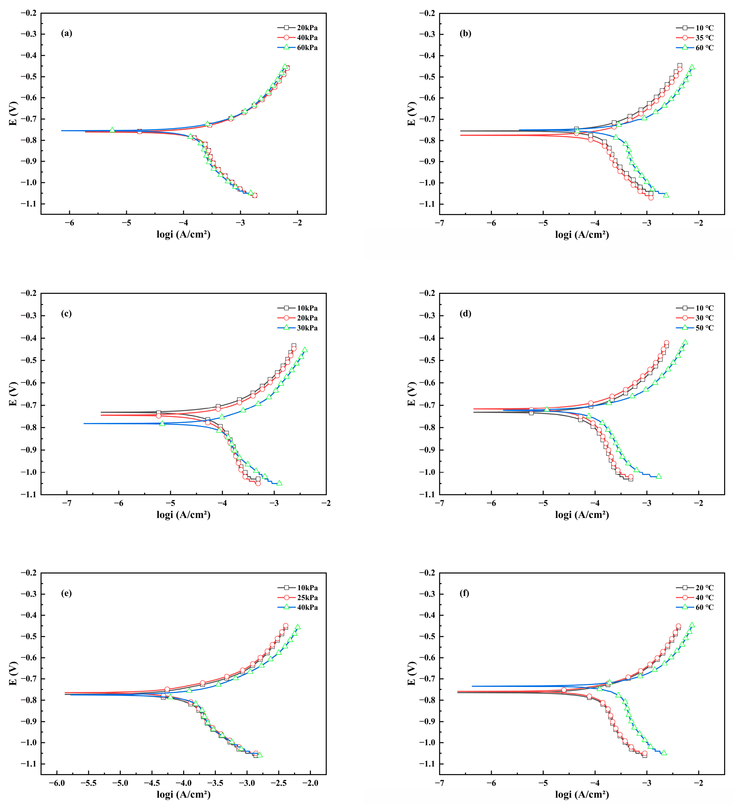
Figure 2: Polarization curves of L360, 20# and X65 steels at different CO2 partial pressures and temperatures. Panels (a,c,e) correspond to different CO2 partial pressures, whereas panels (b,d,f) correspond to different temperatures.
Fig. 3 shows the electrochemical impedance spectra of the three steels under the selected conditions. The Nyquist plots were characterized mainly by depressed capacitive arcs, and the Bode plots showed broad phase-angle peaks, indicating charge-transfer and electric-double-layer responses accompanied by surface heterogeneity. No pronounced long-tail diffusion feature was observed. Because equivalent-circuit fitting was not performed, the EIS data are used qualitatively to compare relative electrochemical trends and are not treated as an independent corrosion-rate dataset.
With increasing CO2 partial pressure, the Nyquist capacitive-arc radius and low-frequency impedance modulus of the three materials generally decreased, reflecting a decrease in interfacial polarization resistance. According to the general interpretation of EIS, lower polarization resistance usually corresponds to higher corrosion current density and poorer corrosion resistance, which is consistent with the polarization curves in Fig. 2 and the weight-loss data in Table 2. This result further confirms that CO2 partial pressure is an important driving factor for static corrosion [1,3,4].
Increasing temperature also reduced the impedance level, indicating that heating weakened the interfacial reaction resistance and accelerated charge transfer. Together with the polarization and weight-loss results, the static corrosion behavior is internally consistent: CO2 partial pressure mainly strengthens the cathodic process by increasing the concentration of carbonate-system reactants, whereas temperature mainly increases the overall corrosion rate by accelerating reaction kinetics.
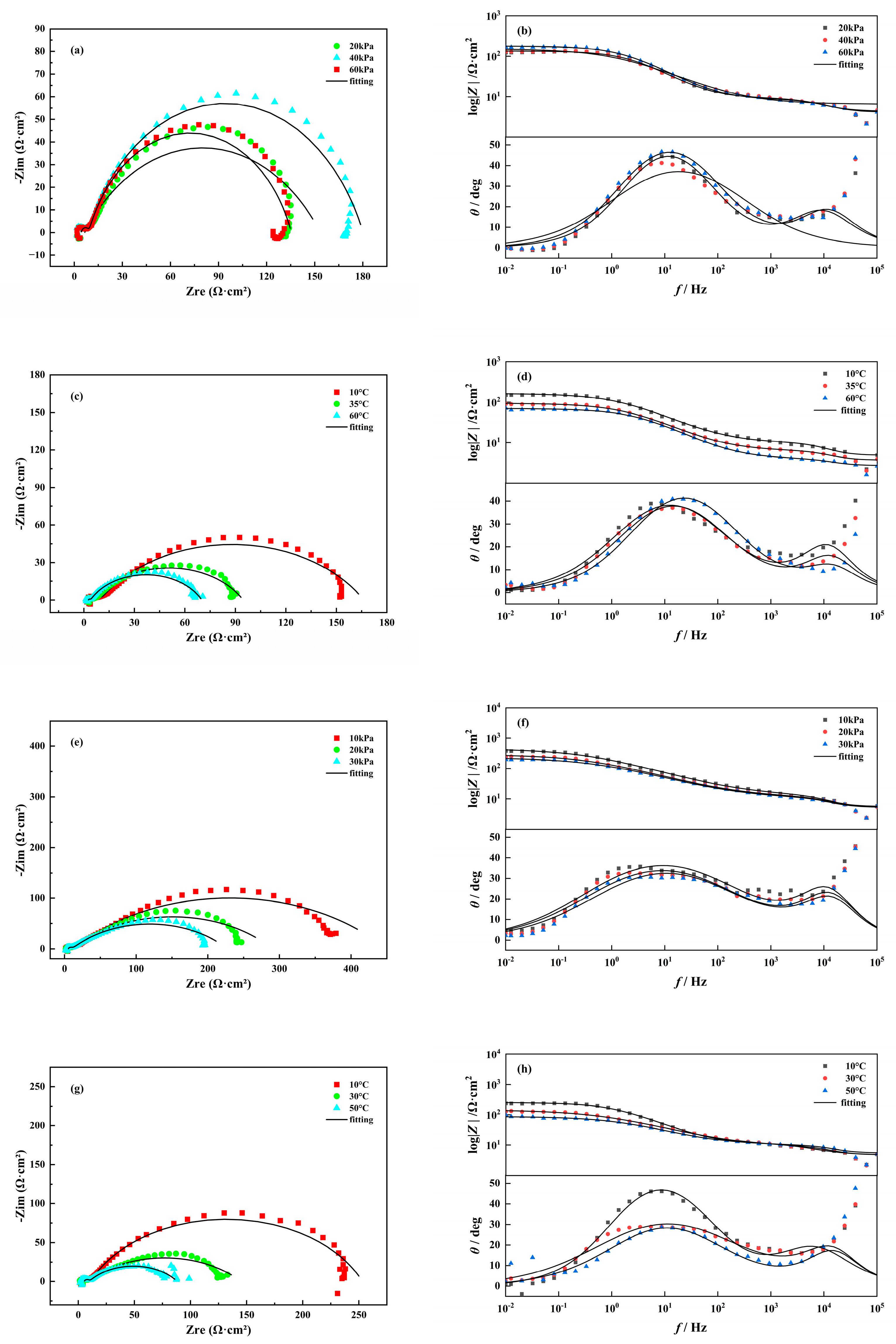
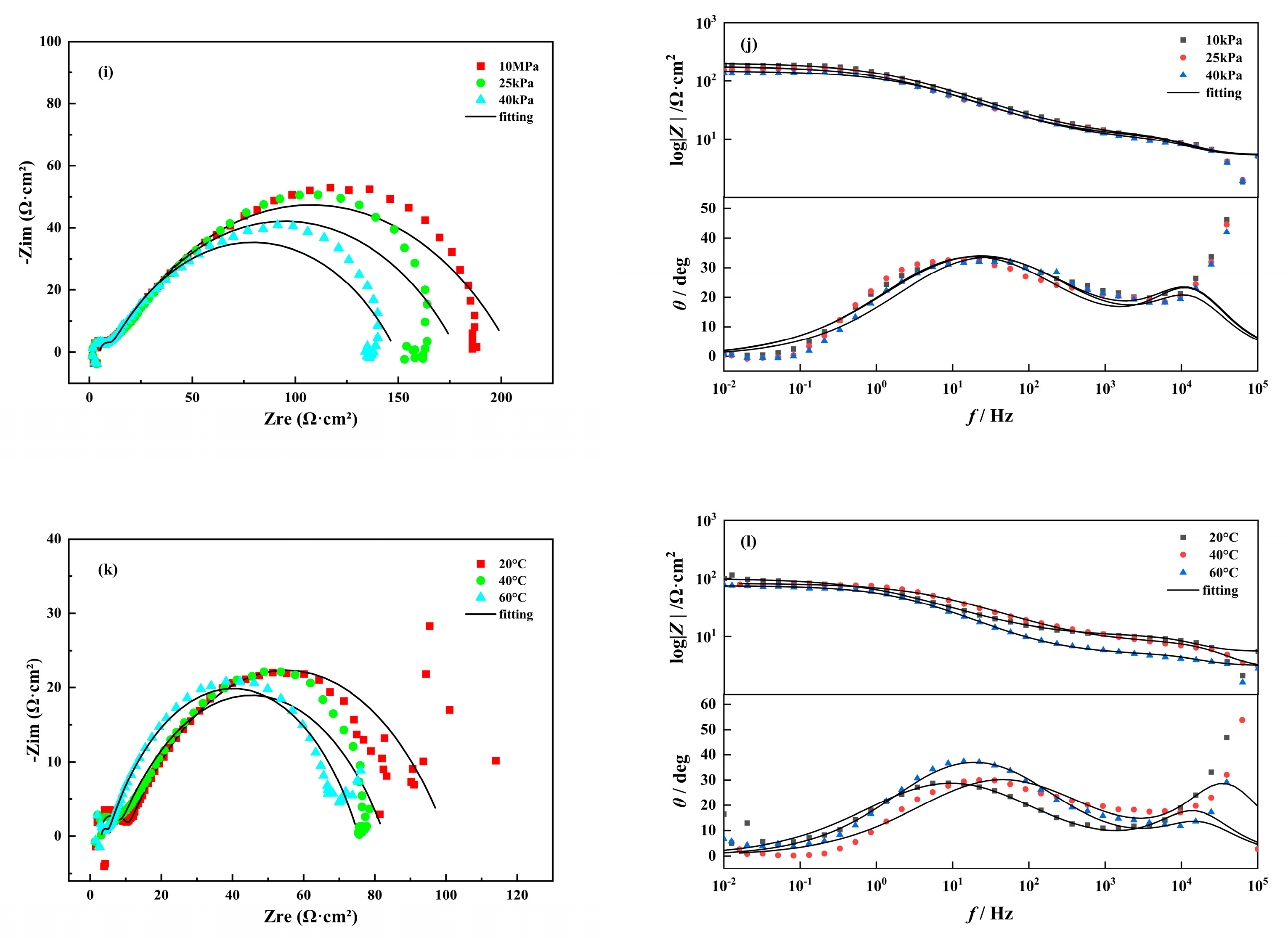
Figure 3: Electrochemical impedance spectra of L360, 20# and X65 steels at different CO2 partial pressures and temperatures. The left panels show Nyquist plots, and the right panels show Bode plots. Panels (a,b,e,f,i,j) correspond to CO2-partial-pressure series, whereas panels (c,d,g,h,k,l) correspond to temperature series. Test conditions are labeled using total pressure P (MPa), CO2 partial pressure PCO2 (kPa) and temperature T (°C).
3.3 Effects of Flow Velocity and Impingement Angle
According to the dynamic erosion-corrosion results listed in Table 3, the corrosion rates of the three materials did not increase monotonically with flow velocity. At an impingement angle of 45°, the rate decreased at low velocity and then increased again at higher velocity. Because the velocity series and angle series were conducted as separate test sequences, their nominally repeated center conditions are identified in the table note below. The trend is therefore interpreted as an apparent response within the specified apparatus and test matrix, not as a universal material ranking.
Table 3: Corrosion rates of the three pipeline steels under static and dynamic conditions.
| Material | Flow Velocity (m/s) | Impingement Angle (°) | Pressure (MPa) | CO2 Partial Pressure (kPa) | Temperature (°C) | Corrosion Rate (mm/a) |
|---|---|---|---|---|---|---|
| L360 | 0 | 0 | 3.5 | 40 | 25 | 0.6002 |
| L360 | 20 | 45 | 3.5 | 40 | 25 | 0.3038 |
| L360 | 30 | 45 | 3.5 | 40 | 25 | 0.3323 |
| L360 | 40 | 45 | 3.5 | 40 | 25 | 0.3470 |
| L360 | 30 | 10 | 3.5 | 40 | 25 | 0.2608 |
| L360 | 30 | 45 | 3.5 | 40 | 25 | 0.3323 |
| L360 | 30 | 80 | 3.5 | 40 | 25 | 0.2920 |
| 20# | 0 | 0 | 3.5 | 40 | 25 | 0.4955 |
| 20# | 30 | 45 | 3.5 | 40 | 25 | 0.2471 |
| 20# | 40 | 45 | 3.5 | 40 | 25 | 0.4647 |
| 20# | 50 | 45 | 3.5 | 40 | 25 | 0.4846 |
| 20# | 40 | 10 | 3.5 | 40 | 25 | 0.3255 |
| 20# | 40 | 45 | 3.5 | 40 | 25 | 0.4647 |
| 20# | 40 | 80 | 3.5 | 40 | 25 | 0.3857 |
| X65 | 0 | 0 | 3.5 | 40 | 25 | 0.6241 |
| X65 | 20 | 45 | 3.5 | 40 | 25 | 0.4753 |
| X65 | 30 | 45 | 3.5 | 40 | 25 | 0.5845 |
| X65 | 40 | 45 | 3.5 | 40 | 25 | 0.5896 |
| X65 | 40 | 10 | 3.5 | 40 | 25 | 0.3011 |
| X65 | 40 | 45 | 3.5 | 40 | 25 | 0.5845 |
| X65 | 40 | 80 | 3.5 | 40 | 25 | 0.3441 |
At low to moderate flow velocities, redistribution of corrosion products and loose deposits may temporarily increase the covered surface fraction and reduce the effective reaction area. Because surface coverage was not measured directly as a function of velocity, this interpretation is phenomenological. At higher velocities, increased wall shear, particle impingement and liquid-flow impact promote deposit removal and expose fresh metal, producing an apparent transition from coverage-related mitigation to erosion-enhanced corrosion.
At an impingement angle of 10°, particle motion is dominated by tangential sliding and shallow-angle micro-cutting. Increasing the angle strengthens the normal impact component, while the cutting efficiency decreases as the trajectory approaches normal incidence. The largest apparent combined damage occurred at 45° in the present apparatus, consistent with established erosion behavior of ductile materials [26,27,28,29,30]. The tests do not, however, provide separate quantitative contributions from mechanical erosion and electrochemical corrosion.
Therefore, both a velocity function and an angle function must be introduced in the subsequent model; dynamic corrosion cannot be described using flow velocity alone.
SEM was used to characterize surface and cross-sectional morphology, including corrosion-product distribution, surface relief, localized features, apparent layer thickness and interfacial bonding. EDS was used for qualitative and semi-quantitative elemental analysis and elemental distribution in selected corrosion-product regions. EDS identifies elements and their spatial distribution but does not independently identify crystalline phases; no phase assignment is made from EDS alone. Representative post-exposure specimens of each steel were selected for SEM/EDS characterization under the conditions shown in Fig. 4, Fig. 5 and Fig. 6. The observations were used to compare corrosion-product morphology and elemental distribution under these selected conditions and were not extrapolated to the entire experimental matrix. The nominal bulk compositions of the steels before exposure are listed in Table 1.
As shown in Fig. 4, at a CO2 partial pressure of 40 kPa and a temperature of 25°C, corrosion products accumulated locally and were relatively dense but non-uniformly distributed. The product crystals were mainly flake-like or layered and existed as overlapping and interlaced structures. This morphology suggests that product growth tended toward two-dimensional extension and did not fully develop into coarse three-dimensional spherical crystals. The EDS sum spectrum in Table 4 showed 91.3 wt% Fe, 4.9 wt% C and 3.7 wt% O, with no detectable Cl. These values describe a selected near-surface corrosion-product region and are therefore not expected to equal the nominal bulk Fe balance reported in Table 1.
As shown in Fig. 5, at a CO2 partial pressure of 30 kPa and a temperature of 25°C, the corrosion products were relatively uniformly distributed but formed a loose and porous layer. Multiple through-thickness cracks indicate limited mechanical stability and a tendency for detachment under fluid and particle impact. The EDS elemental map shows enrichment of O and C together with a weaker Fe signal in product-covered regions, consistent with the morphology observed by SEM. The EDS sum spectrum in Table 5 showed 82.8 wt% Fe, 12.4 wt% C, 4.7 wt% O and 0.1 wt% Cl. These values describe a selected near-surface corrosion-product region rather than the nominal bulk composition listed in Table 1.
Fig. 6 shows a stepped surface morphology, indicating spatially non-uniform corrosion and preferential local dissolution. The observed relief is consistent with repeated formation, damage and detachment of corrosion products. At a CO2 partial pressure of 40 kPa and 25°C, the product layer did not prevent continued non-uniform dissolution. The EDS sum spectrum in Table 6 gave 92.9 wt% Fe, 4.6 wt% C and 2.5 wt% O, with no detectable Cl. These values describe a selected near-surface corrosion-product region and therefore have a different basis from the nominal bulk composition listed in Table 1.
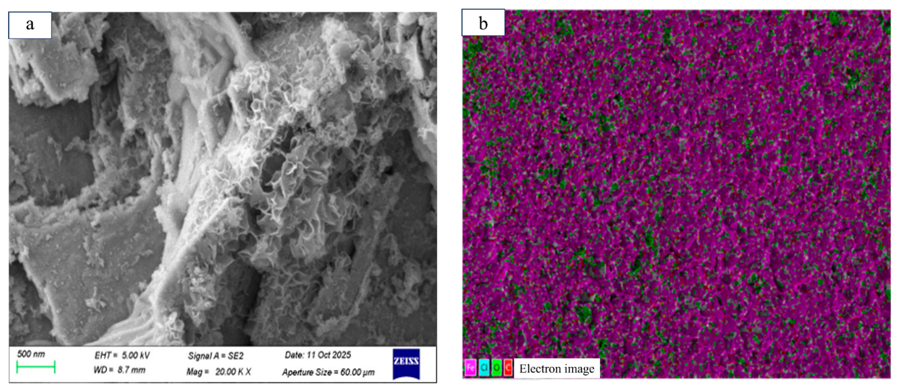
Figure 4: Surface morphology (a) and EDS elemental map (b) of L360 steel at PCO2 = 40 kPa and T = 25°C, 20,000×.
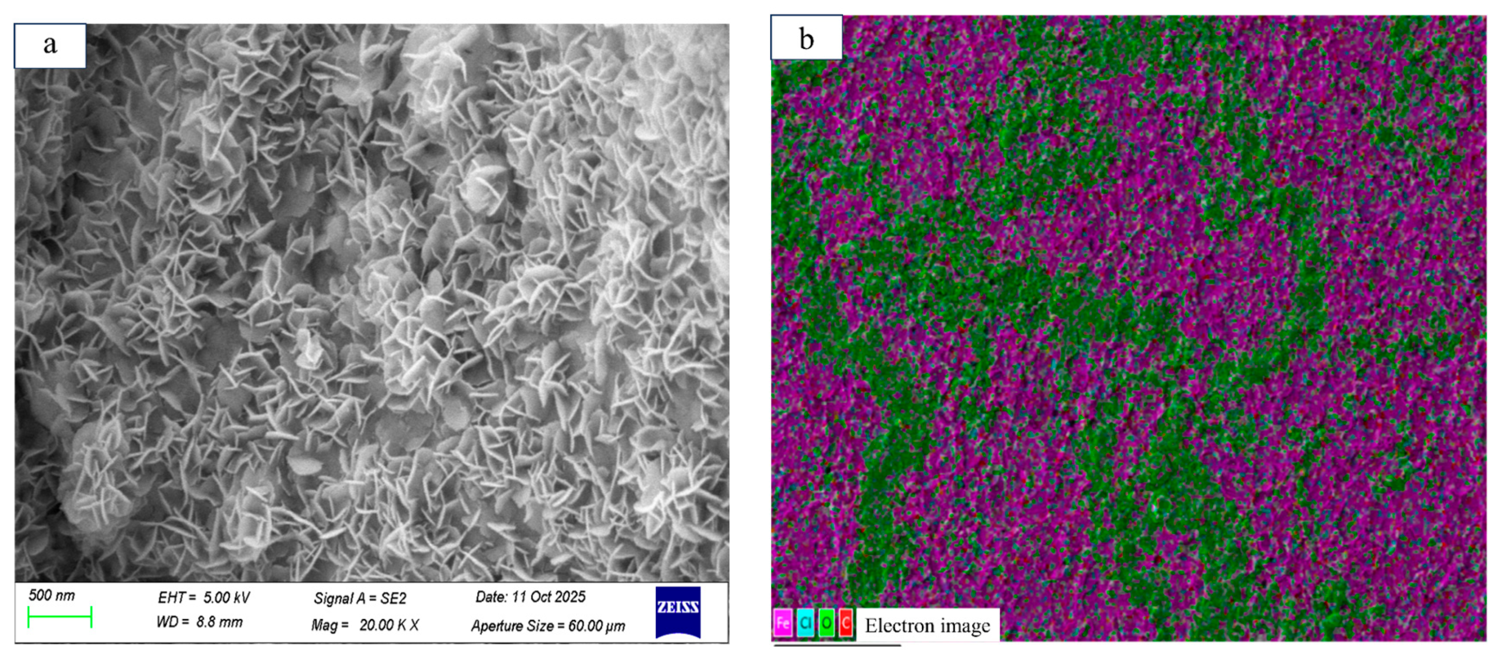
Figure 5: Surface morphology (a) and EDS elemental map (b) of 20# steel at PCO2 = 30 kPa and T = 25°C, 20,000×.
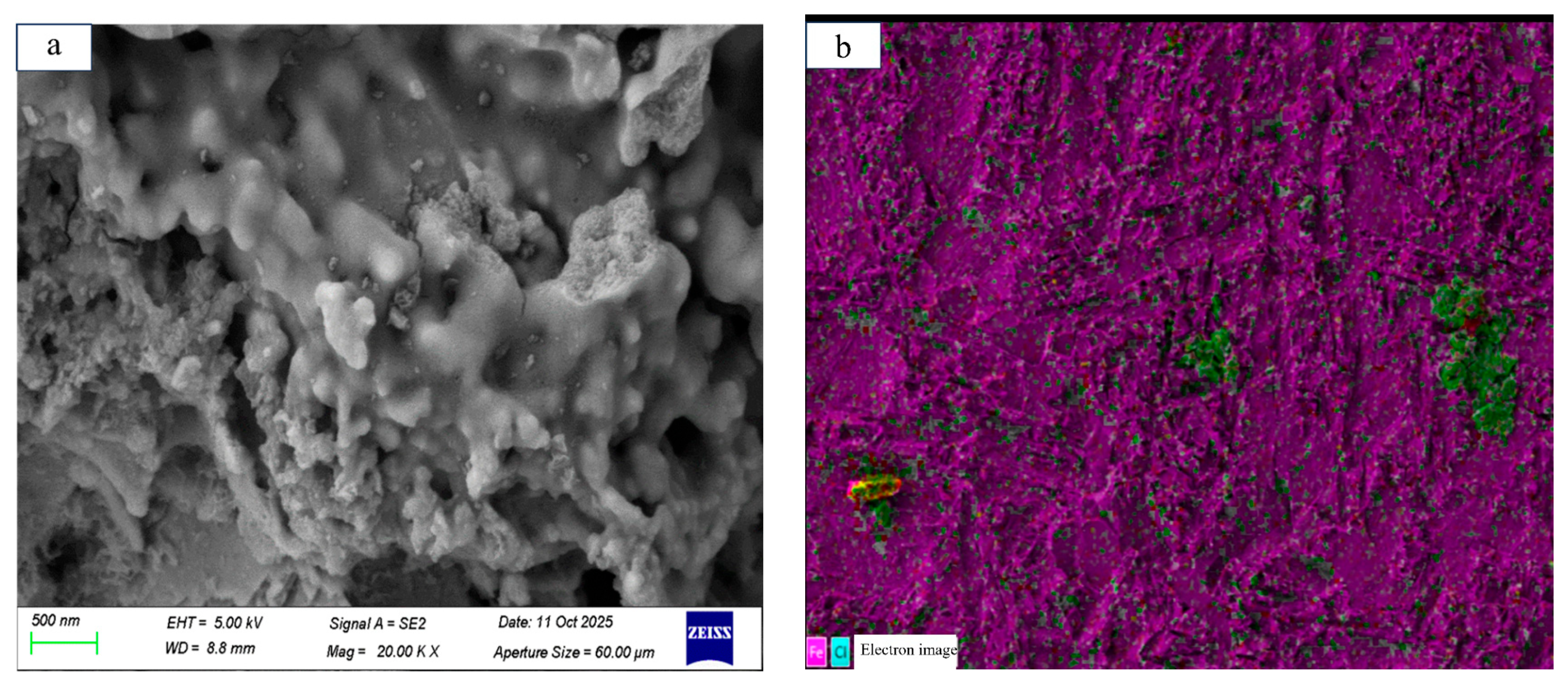
Figure 6: Surface morphology (a) and EDS elemental map (b) of X65 steel at PCO2 = 40 kPa and T = 25°C, 20,000×.
Table 4: Sum Spectrum from Mapping.
| Element | Wt (%) | Standard Deviation (σ) |
|---|---|---|
| Fe | 91.3 | 0.3 |
| C | 4.9 | 0.2 |
| O | 3.7 | 0.1 |
| Cl | 0 | 0.1 |
Table 5: Sum Spectrum from Mapping.
| Element | Wt (%) | Standard Deviation (σ) |
|---|---|---|
| Fe | 82.8 | 0.3 |
| C | 12.4 | 0.2 |
| O | 4.7 | 0.2 |
| Cl | 0.1 | 0.1 |
Table 6: Sum Spectrum from Mapping.
| Element | Wt (%) | Standard Deviation (σ) |
|---|---|---|
| Fe | 92.9 | 0.2 |
| C | 4.6 | 0.2 |
| O | 2.5 | 0.1 |
| Cl | 0 | 0.1 |
The EDS results describe the elemental composition and spatial distribution of selected corrosion-product regions but do not identify crystalline phases. The products are therefore discussed in terms of morphology, elemental distribution and apparent surface coverage without assignment to a specific FeCO3 phase. Definitive phase identification would require complementary X-Ray Diffraction (XRD), Raman spectroscopy or X-ray Photoelectron Spectroscopy (XPS) measurements. Consequently, the coverage term represents the observed corrosion-rate reduction phenomenologically and does not describe FeCO3 film-growth kinetics.
Model development was performed in two stages: static modeling and dynamic correction. The static model was used to describe the controlling effects of temperature, CO2 partial pressure, and pH on corrosion rate under non-flowing and non-erosive conditions. The dynamic correction model was further established on the basis of the static corrosion rate
The de Waard-Milliams model is one of the most widely used baseline models for CO2 corrosion prediction. Its core concept is to describe the reaction-controlled corrosion rate under non-protective-film conditions using temperature and CO2 partial-pressure terms [3,4]. This model type was therefore adopted as the static corrosion baseline. Eqs. (2) and (3) describe the basic relationship between the static corrosion rate and the environmental variables.
4.2 Static-Model Fitting and Coupled Correction for Flow, Surface Coverage, and Erosion
The surface-coverage effect is defined operationally as the apparent reduction in effective reaction area and the increase in interfacial mass-transfer resistance associated with corrosion products, loose deposits and local coverage. Because coverage was not measured directly at different velocities and a continuous compact FeCO3 film was not established, the exponential-saturation term provides an empirical representation of low-velocity mitigation rather than a verified film-growth law.
On the basis of the static model, the corrosion rate under flowing conditions was further corrected. Table 3 shows that increasing flow velocity does not necessarily result in a monotonic increase in corrosion rate; instead, the rate decreases at low velocity and increases again at high velocity. Therefore, the dynamic model cannot rely solely on the mass-transfer enhancement term used in the DW95 or NORSOK models. Surface-coverage-induced deceleration and erosion-damage-induced acceleration must also be explicitly represented.
The three steels differ in composition and were tested in different material-specific static environmental ranges. Their static corrosion sensitivities are therefore interpreted within each material’s own test window rather than compared as if all factors were identical. To avoid forcing material-dependent differences into one parameter set, the static corrosion parameters of L360, 20# and X65 steels were fitted separately using the same model structure. Table 1 shows relevant compositional differences, including the higher C content of 20# steel (0.21 wt%) and the higher Mn and Mo contents of X65 steel (1.45 and 0.145 wt%, respectively). Section 3.1 also shows different corrosion-rate sensitivities to CO2 partial pressure and temperature within the three material-specific test windows. These compositional and response differences support the use of separate fitted parameter sets rather than one unified material parameter.
Based on the static corrosion trends shown in Fig. 2 and Fig. 3 and Table 2,
Static model for L360 steel
Static model for 20# steel
Static model for X65 steel
The dynamic tests showed the highest measured corrosion rate at an impingement angle of 45°. This angular dependence motivated use of a modified Finnie-type function. The function represents the observed response of the present apparatus rather than independently resolved particle-scale mechanics; particle velocity, impact angle, size, trajectory and rotation can all influence material removal [30,31,32,33,34].
With respect to flow velocity, Table 3 shows that all three materials exhibited a non-monotonic trend in which the corrosion rate first decreased and then increased. The dynamic rate was therefore represented by an apparent surface-coverage mitigation term and an erosion-enhancement term. The critical velocity vc in this formulation is a fitted transition parameter for the present apparatus, particle-size range and medium; it was not independently established by a separate threshold experiment. Eq. (8) gives the basic structure of this semi-empirical correction.
All corrosion-rate terms in Eq. (8) are expressed in mm/a.
In Eq. (9),
In Eq. (10),
Integration of the above equation gives:
Because the experimental duration was fixed and flow promoted corrosion-product coverage,
In Eqs. (11)–(13),
The erosion-acceleration term was formulated using a critical-velocity concept. Below a transition velocity, mechanical removal of surface deposits is limited; above it, the s upercritical velocity term represents increasing removal intensity. Critical erosion and deposition concepts have been widely applied to flowing particle systems [26,35]. For the present fixed apparatus, sand-size distribution, concentration and medium,
After rearrangement and simplification, the following expression is obtained:
For Eqs. (14)–(18),
Substitution of the
The parameters
Where
In Eq. (19),
For Eq. (20), N is the number of observations and the objective has units (mm/a)2. The symbol lg used in Eqs. (4)–(6) denotes the base-10 logarithm.
The static corrosion rate, coverage-mitigation term, supercritical-velocity term and angular function were then coupled, and the dynamic parameters were fitted separately for the three steels by least squares. Eqs. (22)–(24) give the resulting material-specific coupled models for L360, 20# and X65 steels, respectively.
Coupled model for L360 steel
Coupled model for 20# steel
Coupled model for X65 steel
4.3 Model Goodness-of-Fit and Internal Comparison
Model performance was examined using residual distributions, material-specific in-sample agreement and comparison with representative formulations evaluated on the same dynamic dataset. Fig. 7 shows normal P-P plots of standardized residuals for the static models, Fig. 8 compares measured and fitted static corrosion rates, and Fig. 9 compares measured and fitted dynamic rates. These figures are goodness-of-fit diagnostics and do not constitute independent validation.
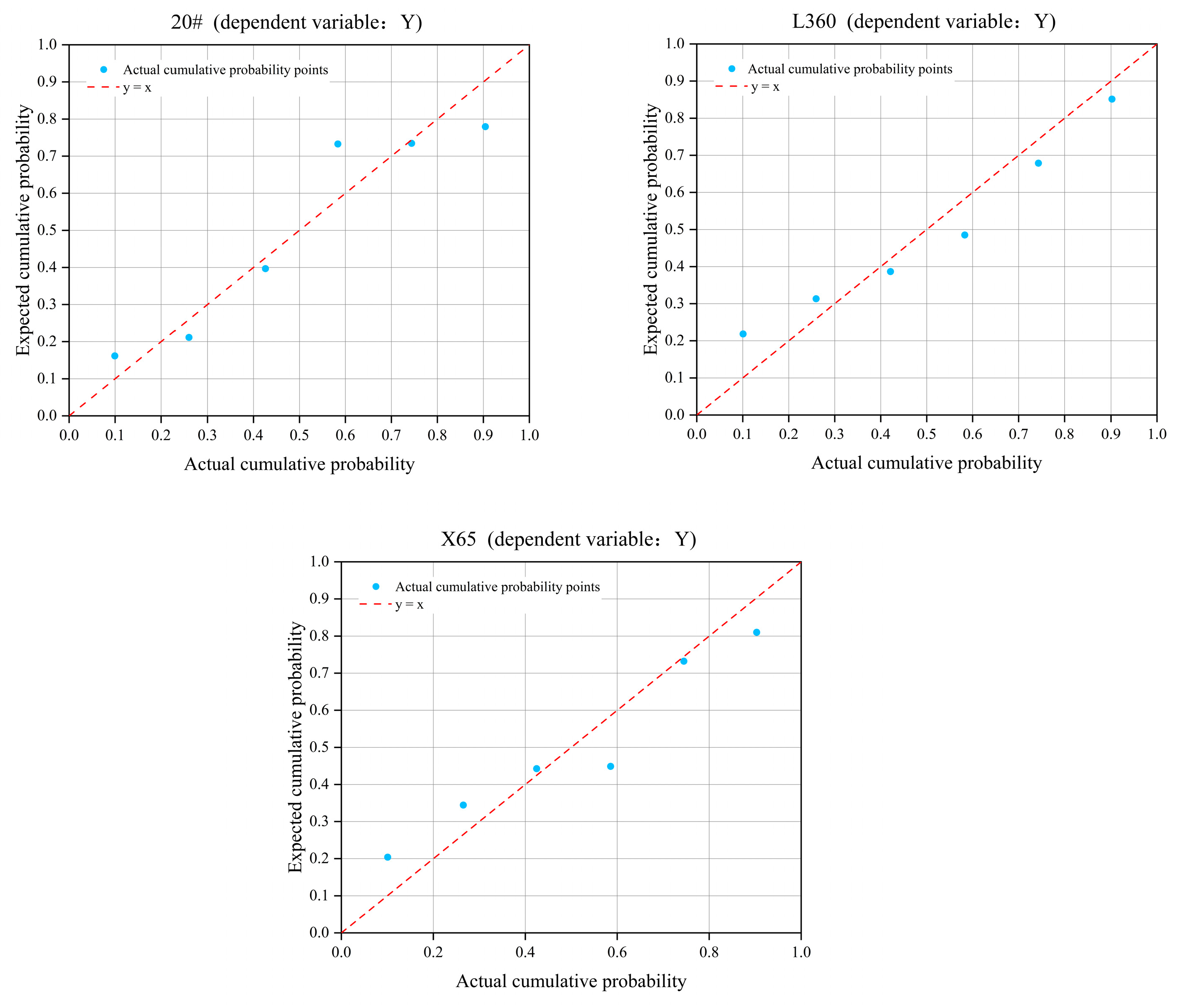
Figure 7: Normal P-P plots of standardized residuals for the material-specific static-model fits.
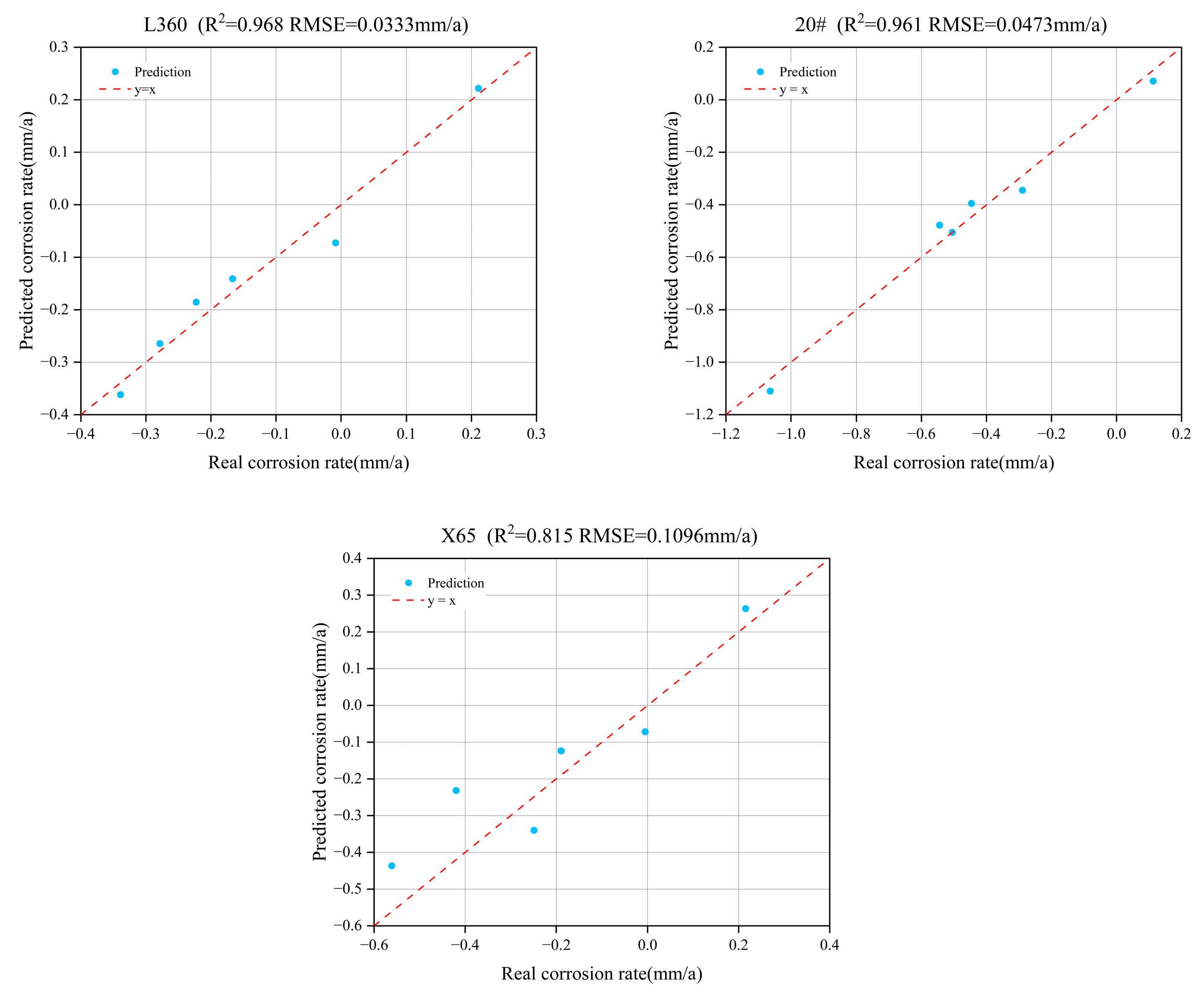
Figure 8: Measured versus fitted corrosion rates for the material-specific static models.
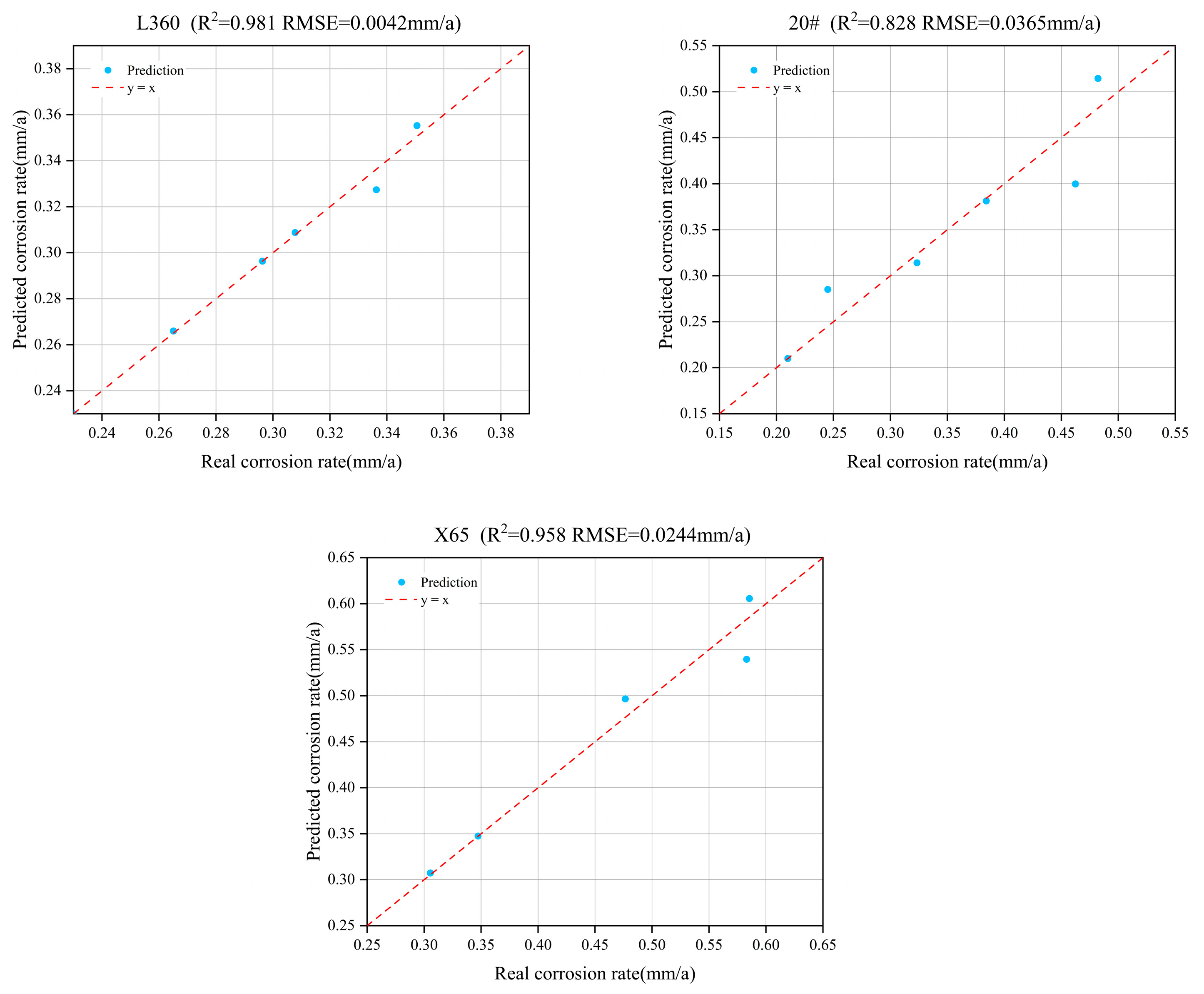
Figure 9: Measured versus fitted dynamic corrosion rates for the coupled models.
To ensure a controlled internal comparison, all benchmark models were evaluated against the same dynamic corrosion data listed in Table 3 using R2 and RMSE. The comparison is therefore an in-sample structural benchmark: it shows how well each formulation describes this dataset under identical metrics, but it does not establish out-of-sample predictive validity. The coupled model includes a static environmental baseline, apparent low-velocity coverage mitigation, high-velocity erosion enhancement and an angular function, which explains its better description of the observed non-monotonic trend. All formulations used the same 21 observations and measured inputs listed in Table 3. Because total pressure, CO2 partial pressure, temperature, salinity and sand loading were fixed in the dynamic matrix, the comparison principally tests how each formulation represents velocity and impingement-angle effects. The quadratic baseline used second-order terms in the dynamic variables; the CFD-shear surrogate represented hydrodynamic loading through a velocity-based shear term; the DW95 and NORSOK references used their respective velocity/shear correction structures; and the film-only model retained the coverage-mitigation term without the erosion contribution. Where coefficient fitting was required, least squares was applied to the same observations without holdout splitting or differential weighting. Thus, Table 7 is a controlled in-sample structural comparison rather than an external validation.
Fig. 10 compares the experimental values with the in-sample predictions from the coupled model and other representative models. The coupled model provided the closest agreement for the present data, and Table 7 lists the corresponding R2 and RMSE values. Because all models were evaluated on the same observations, this result is interpreted as an internal comparison of descriptive performance rather than independent predictive validation.
Table 7: Error comparison of different corrosion prediction models.
| Model | Coupled Model | ML Quadratic Baseline | CFD-Shear Surrogate | DW95 Resistance Model | Film-Only Kinetic Model | NORSOK Shear Reference |
|---|---|---|---|---|---|---|
| R2 | 0.9308 | 0.6338 | 0.6149 | 0.345 | 0.261 | −4.4133 |
| RMSE | 0.0319 | 0.0735 | 0.0754 | 0.0983 | 0.1044 | 0.2826 |
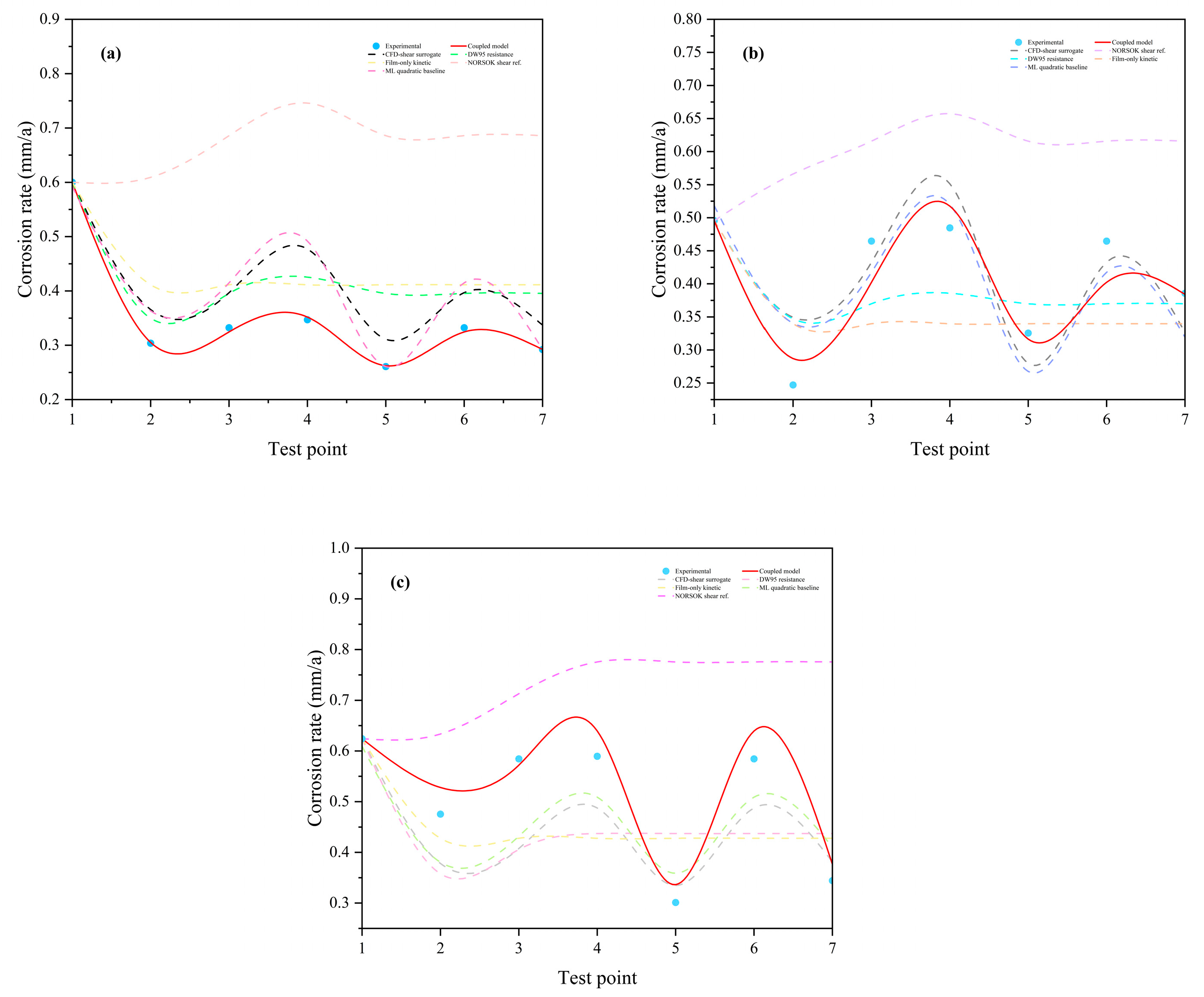
Figure 10: In-sample comparison of experimental values and predictions from the coupled and benchmark models: (a) L360, (b) 20#, and (c) X65.
Although the coupled model achieved R2 = 0.9308 and RMSE = 0.0319 for the present dynamic dataset, these values mainly reflect in-sample explanatory capability. The number of dynamic test samples was limited, and sand-size distribution and concentration, temperature, CO2 partial pressure and medium conditions were relatively fixed. The model is therefore positioned as a material- and apparatus-specific semi-empirical formulation applicable within the tested range; extrapolation to other materials, complex multiphase flow regimes and long-term field operation requires independent validation and recalibration. The internal comparison comprised the 21 observations in Table 3, including the static controls and the separately exposed center conditions from the velocity and angle test sequences.
- 1.Static weight-loss, potentiodynamic polarization and EIS observations showed that the CO2 corrosion rates of L360, 20# and X65 pipeline steels increased overall with increasing CO2 partial pressure and temperature within each material’s experimental range. Increasing CO2 partial pressure mainly enhanced the cathodic reduction process, whereas increasing temperature mainly accelerated interfacial charge transfer and reaction kinetics.
- 2.The dynamic tests showed a non-monotonic corrosion-rate response to flow velocity, with the highest measured rate at an impingement angle of 45° in this apparatus. The observation is represented by apparent surface-coverage mitigation and high-velocity erosion enhancement; separate corrosion, erosion and synergistic contributions were not independently quantified.
- 3.SEM and EDS observations did not establish a crystalline FeCO3-dominated protective film. The film-related term is therefore defined as a generalized surface-coverage/deposit effect, and phase identification would require XRD, Raman spectroscopy or XPS. This conclusion applies to the representative post-exposure conditions shown in Fig. 4, Fig. 5 and Fig. 6 (25°C and CO2 partial pressures of 30–40 kPa) and is not generalized to all static conditions in Table 2.
- 4.The coupled model achieved R2 = 0.9308 and RMSE = 0.0319 on all dynamic observations and provided the best in-sample description among the benchmark formulations. It is a material- and apparatus-specific semi-empirical model constrained by the present experimental matrix, not a universal pipeline-corrosion predictor. Its parameters apply to the tested ranges of pipeline steel grade, CO2 partial pressure, temperature, flow velocity, impingement angle and quartz-sand size distribution and concentration. Conditions involving higher salinity, different pH values, different sand concentrations, complex multiphase flow or long-term field service require new measurements, recalibration and independent validation.
Acknowledgement:
Funding Statement: This work was supported by the Regional Special Support Program of the 77th General Grant of the China Postdoctoral Science Foundation (No. 2025MD774094), the Scientific Research Project of Gansu Provincial Higher Education Institutions (Grant No. 2026QB-033), and the Gansu Provincial Youth Science and Technology Fund for the project “Study on Oil-Water Interfacial Mechanisms and Differential Pressure Behaviors under Multi-Field Coupling” (Project No. 25JRRA910).
Author Contributions: Jiabin Wang and Rundong Wang conducted the experiments and analyzed the data. Xingda Tong conceived and supervised the study. Shaopeng Hao contributed to the methodology and data interpretation. Bo Yan and Zhihui Wang contributed to the discussion and manuscript revision. All authors reviewed and approved the final version of the manuscript.
Availability of Data and Materials: The data generated or analyzed during this study are available from the corresponding authors upon reasonable request.
Ethics Approval: Not applicable.
Conflicts of Interest: The authors declare no conflicts of interest.
References
1. Nešić S . Key issues related to modelling of internal corrosion of oil and gas pipelines—A review. Corros Sci. 2007; 49( 12): 4308– 38. doi:10.1016/j.corsci.2007.06.006. [Google Scholar] [CrossRef]
2. Kahyarian A , Singer M , Nesic S . Modeling of uniform CO2 corrosion of mild steel in gas transportation systems: A review. J Nat Gas Sci Eng. 2016; 29: 530– 49. doi:10.1016/j.jngse.2015.12.052. [Google Scholar] [CrossRef]
3. De Waard C , Milliams DE . Carbonic acid corrosion of steel. Corrosion. 1975; 31( 5): 177– 81. doi:10.5006/0010-9312-31.5.177. [Google Scholar] [CrossRef]
4. de Waard C , Lotz U , Dugstad A . Influence of liquid flow velocity on CO2 corrosion: A semi-empirical model. In: Proceedings of the CORROSION 1995; 1995 Mar 26–31; Orlando, FL, USA. p. 1– 15. doi:10.5006/c1995-95128. [Google Scholar] [CrossRef]
5. NORSOK M-506:2017. CO2 corrosion rate calculation model. 3rd ed. Lysaker, Norway: Standards Norway; 2017. [Google Scholar]
6. Gartland PO , Johnsen R , ∅vstetun I . Application of internal corrosion modeling in the risk assessment of pipelines. In: Proceedings of the CORROSION 2003; 2003 Mar 16–21; San Diego, CA, USA. p. 1– 14. doi:10.5006/c2003-03179. [Google Scholar] [CrossRef]
7. Nordsveen M , Nešić S , Nyborg R , Stangeland A . A mechanistic model for carbon dioxide corrosion of mild steel in the presence of protective iron carbonate films—Part 1: Theory and verification. Corrosion. 2003; 59( 5): 443– 56. doi:10.5006/1.3277576. [Google Scholar] [CrossRef]
8. Nešić S , Lee KJ . A mechanistic model for carbon dioxide corrosion of mild steel in the presence of protective iron carbonate films—Part 3: Film growth model. Corrosion. 2003; 59( 7): 616– 28. doi:10.5006/1.3277592. [Google Scholar] [CrossRef]
9. Shadley JR , Shirazi SA , Dayalan E , Rybicki EF . Prediction of erosion-corrosion penetration rate in a carbon dioxide environment with sand. Corrosion. 1998; 54( 12): 972– 8. doi:10.5006/1.3284819. [Google Scholar] [CrossRef]
10. Kanwar S , Jepson WP . A model to predict sweet corrosion of multiphase flow in horizontal pipelines. In: Proceedings of the CORROSION 1994; 1994 Feb 27–Mar 4; Baltimore, MD, USA. p. 1– 12. doi:10.5006/c1994-94024. [Google Scholar] [CrossRef]
11. Li GH , Gu T , Tang YF , Liu ZD , Wu H , He ZY . CO2 corrosion prediction model. Corros Prot Petrochem Ind. 2007; 6: 1– 4. (In Chinese). [Google Scholar]
12. Zhang ZH , Guo JB . Corrosion of CO2 to oil and gas pipes and research progress at home and abroad. Baogang Technol. 2000; 4: 54– 8. (In Chinese). [Google Scholar]
13. Li F , Wang TY , Guo ZY , Leng CJ , Zheng ZB . Research on corrosion model of CO2 flooding production and transportation components. Petrochem Ind Technol. 2019; 26( 10): 259+261. (In Chinese). [Google Scholar]
14. Remita E , Tribollet B , Sutter E , Vivier V , Ropital F , Kittel J . Hydrogen evolution in aqueous solutions containing dissolved CO2: Quantitative contribution of the buffering effect. Corros Sci. 2008; 50( 5): 1433– 40. doi:10.1016/j.corsci.2007.12.007. [Google Scholar] [CrossRef]
15. Gong ZL , Peng SN , Huang XM , Gao LZ . Development of prediction model of carbon dioxide corrosion rate of natural gas pipeline steel. Gas Heat. 2017; 37( 8): 1– 7. (In Chinese). doi:10.13608/j.cnki.1000-4416.2017.08.010. [Google Scholar] [CrossRef]
16. Barker R , Burkle D , Charpentier T , Thompson H , Neville A . A review of iron carbonate (FeCO3) formation in the oil and gas industry. Corros Sci. 2018; 142: 312– 41. doi:10.1016/j.corsci.2018.07.021. [Google Scholar] [CrossRef]
17. Choi YS , Farelas F , Nešić S , Magalhães AAO , de Azevedo Andrade C . Corrosion behavior of deep water oil production tubing material under supercritical CO2 environment: Part 1—Effect of pressure and temperature. Corrosion. 2014; 70( 1): 38– 47. doi:10.5006/1019. [Google Scholar] [CrossRef]
18. Jiang HJ , Wang ZH , Wang XS , Zhao S , Sun C , Zheng W . Study on CO2 corrosion behavior of L415 pipeline steel in natural gas environment. Hot Work Technol. 2021; 50( 18): 83– 7. (In Chinese). doi:10.14158/j.cnki.1001-3814.20200134. [Google Scholar] [CrossRef]
19. Sk MH , Abdullah AM , Ko M , Ingham B , Laycock N , Arul R , et al. Local supersaturation and the growth of protective scales during CO2 corrosion of steel: Effect of pH and solution flow. Corros Sci. 2017; 126: 26– 36. doi:10.1016/j.corsci.2017.05.026. [Google Scholar] [CrossRef]
20. Di Bonaventura M , Brown B , Nešić S , Singer M . Effect of flow and steel microstructure on the formation of iron carbonate. Corrosion. 2019; 75( 10): 1183– 93. doi:10.5006/3118. [Google Scholar] [CrossRef]
21. Owen J , Godfrey J , Ma W , de Boer G , Al-Khateeb M , Thompson H , et al. An experimental and numerical investigation of CO2 corrosion in a rapid expansion pipe geometry. Corros Sci. 2020; 165: 108362. doi:10.1016/j.corsci.2019.108362. [Google Scholar] [CrossRef]
22. Thorat U , Jones M , Woollam R , Owen J , Barker R , Thompson H , et al. Computational fluid dynamics driven mass transfer model for the prediction of CO2 corrosion in pipelines. J Pipeline Sci Eng. 2024; 4( 1): 100148. doi:10.1016/j.jpse.2023.100148. [Google Scholar] [CrossRef]
23. Yang H , Lu L , Tsai K , Sidahmed M . A hybrid physics and active learning model for CFD-based pipeline CO2 and O2 corrosion prediction. In: Proceedings of the International Petroleum Technology Conference; 2023 Mar 1–3; Bangkok, Thailand. doi:10.2523/iptc-23049-ea. [Google Scholar] [CrossRef]
24. Aghaaminiha M , Mehrani R , Colahan M , Brown B , Singer M , Nesic S , et al. Machine learning modeling of time-dependent corrosion rates of carbon steel in presence of corrosion inhibitors. Corros Sci. 2021; 193: 109904. doi:10.1016/j.corsci.2021.109904. [Google Scholar] [CrossRef]
25. Silakorn P , Jantrakulchai N , Wararatkul N , Wanwilairat S , Kangkachit T , Techapiesancharoenkij R , et al. Top-of-line corrosion via physics-guided machine learning: A methodology integrating field data with theoretical models. J Petrol Sci Eng. 2022; 215: 110558. doi:10.1016/j.petrol.2022.110558. [Google Scholar] [CrossRef]
26. Wang ZB , Zheng YG . Critical flow velocity phenomenon in erosion-corrosion of pipelines: Determination methods, mechanisms and applications. J Pipeline Sci Eng. 2021; 1( 1): 63– 73. doi:10.1016/j.jpse.2021.01.005. [Google Scholar] [CrossRef]
27. Finnie I . Erosion of surfaces by solid particles. Wear. 1960; 3( 2): 87– 103. doi:10.1016/0043-1648(60)90055-7. [Google Scholar] [CrossRef]
28. Bitter JGA . A study of erosion phenomena part I. Wear. 1963; 6( 1): 5– 21. doi:10.1016/0043-1648(63)90003-6. [Google Scholar] [CrossRef]
29. Bitter JGA . A study of erosion phenomena: Part II. Wear. 1963; 6( 3): 169– 90. doi:10.1016/0043-1648(63)90073-5. [Google Scholar] [CrossRef]
30. Oka YI , Yoshida T . Practical estimation of erosion damage caused by solid particle impact. Wear. 2005; 259( 1–6): 102– 9. doi:10.1016/j.wear.2005.01.040. [Google Scholar] [CrossRef]
31. Zhao X , Cao X , Zhang J , Cao H , Zhang J , Peng W , et al. Experimental and numerical investigation of erosion in plugged tees for liquid-solid flow. Int J Multiph Flow. 2023; 160: 104348. doi:10.1016/j.ijmultiphaseflow.2022.104348. [Google Scholar] [CrossRef]
32. Zhao X , Cao X , Xie Z , Cao H , Wu C , Bian J . Numerical study on the particle erosion of elbows mounted in series in the gas-solid flow. J Nat Gas Sci Eng. 2022; 99: 104423. doi:10.1016/j.jngse.2022.104423. [Google Scholar] [CrossRef]
33. Zhao X , Cao X , Cao H , Zhang J , Zhang J , Peng W , et al. Numerical study of elbow erosion due to sand particles under annular flow considering liquid entrainment. Particuology. 2023; 76: 122– 39. doi:10.1016/j.partic.2022.07.006. [Google Scholar] [CrossRef]
34. Zang X , Cao X , Zhang J , Xie Z , Xiong N , Darihaki F , et al. Investigation of surface damage of ductile materials caused by rotating particles. Wear. 2022; 488: 204185. doi:10.1016/j.wear.2021.204185. [Google Scholar] [CrossRef]
35. Partheniades E . Erosion and deposition of cohesive soils. J Hydr Div. 1965; 91( 1): 105– 39. doi:10.1061/jyceaj.0001165. [Google Scholar] [CrossRef]
Cite This Article
 Copyright © 2026 The Author(s). Published by Tech Science Press.
This work is licensed under a Creative Commons Attribution 4.0 International License , which permits unrestricted use, distribution, and reproduction in any medium, provided the original work is properly cited.
 Downloads
 Citation Tools
