
 Login
Login Register
 Submit a Paper
 Propose a Special lssue
 Open Access
ARTICLE
Sequential Modeling of Liquid Hydrogen Leakage, Dispersion and Post-Ignition Thermal Hazards in Semi-Open Railway Stations
1 CRRC Academy (Qingdao) Co., Ltd., Qingdao, China
2 College of Automotive and Energy Engineering, Tongji University, Shanghai, China
3 School of Civil Engineering and Architecture, Hebei University of Engineering Science, Shijiazhuang, China
4 Hebei Key Laboratory of Cryogenic Energy Storage, School of Mechanical Engineering, Shijiazhuang Tiedao University, Shijiazhuang, China
5 Beijing Xingyou Engineering Project Management Co., Ltd., Beijing, China
6 College of Chemical Engineering, Fuzhou University, Fuzhou, China
* Corresponding Authors: Yuejiao Wang. Email: ; Pengbo Yin. Email:
Fluid Dynamics & Materials Processing 2026, 22(9), 8 https://doi.org/10.32604/fdmp.2026.089244
Received 16 July 2026; Accepted 09 September 2026; Issue published 28 September 2026
 View Full Text
 Download PDF
Abstract
This study develops a sequential numerical modelling framework to elucidate the transient evolution of liquid hydrogen (LH2) leakage, pool evaporation, hydrogen dispersion, and post-ignition thermal hazards in a representative semi-open railway station. The framework couples a source-term integral model for LH2 pool evaporation with computational fluid dynamics (CFD), in which the time-dependent liquid-pool radius and evaporation mass flow rate are introduced as transient inlet conditions through a user-defined function. The Realizable k-ε turbulence model and species transport equations are employed to predict the subsequent dispersion of gaseous H2 within the station environment, accounting for the influence of large-span roofs, locomotives, and structural columns on hydrogen migration and retention. At 3.0 s after leakage initiation, the analysis branches into non-ignited dispersion and ignition/combustion scenarios. For the latter, the instantaneous H2 concentration, temperature, and velocity fields are used to initialize ignition at (−0.7, −3.6, 0.5) m. The results show that the LH2 evaporation mass flow rate reaches approximately 3.6 kg/s at 3.7–3.8 s, while the liquid-pool radius increases to approximately 1.2 m at 4.2 s. In the non-ignited scenario, the 4 vol% H2 cloud reaches a front position of 22.42 m and a length of 28.92 m at 9 s, while residual hydrogen continues to migrate and dilute for approximately 200 s. In the ignition/combustion scenario, the maximum flame temperature reaches 2193.5 K at 3.0 s. The combustion analysis is limited to post-ignition thermal effects and does not consider deflagration-induced overpressure or structural response.Keywords
Hydrogen-powered transportation is an important pathway for deep decarbonization in the transport sector and has attracted increasing attention in rail transit systems. Liquid hydrogen (LH2), with its high volumetric energy density, high storage and transport efficiency, and rapid refueling capability, is considered a promising energy-storage form for future medium- and long-distance hydrogen fuel-cell locomotives. It can greatly improve driving range within limited onboard space and can serve as a clean-energy alternative for non-electrified railway lines [1,2,3]. However, during external refueling, parking, or maintenance, a rupture-induced leakage in the LH2 storage and supply system may rapidly release ultra-low-temperature LH2 onto the ground outside the station, forming a cryogenic liquid pool. The pool then evaporates continuously under ground heat transfer, air convection, and radiation, forming a low-temperature H2 cloud. This process involves coupled physical phenomena, including pool spreading, phase-change evaporation, buoyancy-driven migration, turbulent mixing, and flammable-cloud evolution. As a result, accident consequences show strong transient behavior and spatial non-uniformity [4,5,6,7].
In addition to cryogenic hazards, H2 has a wide flammability range, low ignition energy, and high diffusivity, which leads to a high fire and explosion risk after mixing with air [8]. In semi-open spaces such as stations, the early H2 cloud is mainly controlled by inertia and ambient wind and disperses downwind. As its density decreases, buoyancy gradually becomes dominant, and local retention zones may form beneath the roof, around the locomotive, and in the leeward regions of structures. When the concentration enters the flammable range and an ignition source is present, rapid combustion or even deflagration may occur. Station roofs, parked locomotives, support columns, and other obstacles further alter the flow field, making hydrogen-cloud migration paths and hazardous-zone distributions more complex [9,10].
Current studies on hydrogen and LH2 leakage, dispersion, and combustion mainly use experimental methods and numerical simulations, covering both open and confined-space scenarios. In experiments, high-pressure hydrogen release tests have been used to analyze the effects of leak diameter, pressure, and ambient wind on dispersion behavior [11,12,13]. For example, Niu et al. [14] found that concentration decay in hydrogen jets shows a degree of self-similarity, whereas turbulence induced by ambient wind and obstacles can significantly change far-field concentration distributions and cause local accumulation. However, due to safety and scale limitations, full-scale LH2 leakage experiments remain limited, and equivalent studies often rely on substitute gases or scaled experiments [15]. In numerical simulations, CFD and commercial software such as PHAST have been widely applied to open-space and hydrogen-refueling-station scenarios to simulate hydrogen leakage, dispersion, and combustion [16,17,18,19]. Zhang et al. [20] used CFD coupled with a k-ε turbulence model and a combustion model to study hydrogen leakage and combustion in fuel-cell bus maintenance workshops, showing that leakage location, leak diameter, and ventilation wind speed significantly affect flammable-cloud accumulation, jet-fire behavior, heat-release duration, and workshop safety design. These studies usually couple multiphase flow, turbulent transport, and combustion models to predict hydrogen-cloud concentration fields, temperature fields, and the evolution of flammable regions. For example, in LH2 refueling station scenarios, barrier-structure parameters can markedly influence downwind expansion and vertical migration of hydrogen clouds, and proper design can effectively reduce the flammable-cloud range and cryogenic impact zone [11,21,22]. However, these studies mainly focus on open or semi-open industrial facilities, whose boundary conditions differ clearly from those of station spaces.
For confined spaces, existing studies mainly focus on tunnels, underground garages, and enclosed industrial buildings. The results show that spatial scale, ventilation mode, and obstacle distribution significantly affect upper-layer accumulation, recirculation structures, and combustion intensity of hydrogen clouds [23,24,25,26]. Xu et al. [27] conducted experimental and numerical studies on hydrogen leakage and dispersion in large-aspect-ratio spaces and identified three typical dispersion stages, including buoyancy-dominated rise, horizontal spreading, and vertical filling, showing that leakage rate and direction significantly affect dispersion time and concentration distribution and providing a basis for warning-threshold and emergency-strategy design. Li et al. [28] analyzed leakage accidents of hydrogen-powered vehicles in parking garages and showed that leakage amount, ventilation-opening arrangement, exhaust-fan operation, and partition-wall layout jointly affect hydrogen dispersion and retention risks. Their findings provide a reference for hydrogen-safety ventilation design and risk control in parking garages. Chen et al. [29] analyzed high-pressure hydrogen leakage and dispersion from hydrogen fuel-cell trains in tunnels and found that leakage direction, hole diameter, and train speed strongly affect hydrogen accumulation risk. When the train speed is not lower than 40 km/h, the piston-wind effect can effectively suppress hydrogen accumulation between the train roof and tunnel ceiling. Overall, recirculating airflow, roof confinement, and obstacle-induced flow in confined or semi-confined spaces can enhance local turbulent mixing, change the spatial distribution of flammable clouds, and promote flame acceleration. However, rail transit stations usually have semi-open boundaries, large-span roofs, support columns, and parked locomotives. Their ventilation organization, buoyancy-driven migration paths, and hydrogen-cloud retention mechanisms differ from those of tunnels, underground garages, and enclosed buildings. Existing studies are therefore insufficient to reveal the coupling mechanisms among liquid-pool evaporation, hydrogen-cloud migration, obstacle disturbance, and flame propagation after LH2 leakage in station scenarios.
Existing studies on LH2 leakage have mainly considered open environments, hydrogen refueling stations, and tunnels, whereas semi-open large spaces such as railway stations have received relatively limited attention. In addition, dispersion and combustion are often investigated separately, and the combined effects of liquid-pool evaporation, low-temperature H2 cloud dispersion, station structures, flammable-cloud distribution, and post-ignition flame development have not been extensively examined within an integrated station scenario. In railway stations, roofs, locomotives, and support columns may influence the upward and lateral transport of released H2 and contribute to spatial variations in local hydrogen accumulation. Therefore, this study considers a representative LH2-release scenario in a semi-open railway station under prescribed release, ventilation, and geometric conditions. The analysis focuses on the temporal and spatial evolution of the H2 cloud from the release region to the upper station space, the local influence of the locomotive and support columns on hydrogen distribution, and the development of dispersion-related and post-ignition thermal-hazard regions. The results provide a scenario-specific evaluation of LH2 leakage and ignition behavior under the selected station configuration and operating conditions, rather than a generalized parametric description of LH2 release characteristics.
2 Numerical Model and Methodology
2.1 Physical Properties and Theoretical Model
During operation, parking, or refueling of a liquid-hydrogen fuel-cell locomotive, an integrity failure of cryogenic storage tanks, connecting pipelines, valves, or safety accessories may cause LH2 to be rapidly released onto the ground and form a cryogenic liquid pool. The catastrophic rupture considered in this study refers to abnormal loss of integrity in the hydrogen storage system, causing a large amount of LH2 to be released in an uncontrolled manner. It is not a controllable release such as a small-hole leakage or safety-valve discharge. Although such accidents have a relatively low probability, they are typical high-consequence events. After the cryogenic liquid is released, it undergoes liquid-pool expansion, intense evaporation, H2-air mixing, flammable-cloud formation, and ignition combustion, which may cause cryogenic injury, fire, and local high-temperature impact. In this study, a 6 kg LH2 release is selected as the representative accident condition. This release amount is determined with reference to reported hydrogen inventory requirements for hydrogen-powered vehicles; for example, approximately 5.6 kg of LH2 can support a hydrogen-powered passenger vehicle over a driving range of about 350 miles. Considering that the onboard hydrogen storage capacity of a fuel-cell locomotive is expected to be larger than that of a passenger vehicle, the 6 kg release scenario is used as a conservative representative case for evaluating leakage, dispersion, and combustion hazards of the locomotive LH2 storage system in a semi-open station space [30].
The physical properties of LH2, H2, and air are the basis for source-term calculation and CFD simulation. In the source-term integral model, LH2 is treated as a cryogenic liquid medium. Its saturation temperature, liquid density, latent heat of vaporization, constant-pressure specific heat, and thermal conductivity are used to describe pool formation and heat-induced evaporation after leakage. The phase-change temperature of LH2 is set to 20.3 K to determine the inlet temperature after evaporation into the gas phase. In the CFD model, gaseous H2 and air are treated as miscible gas species. The density of the H2-air mixture is calculated using the ideal-gas equation of state and updated with local temperature and species mass fraction. Transport properties, including viscosity, specific heat capacity, thermal conductivity, and diffusion coefficient, are assigned according to material properties or temperature-dependent parameters. This treatment can reflect the warming, buoyancy variation, and mixing dispersion of low-temperature H2 after it enters the environment. The properties of H2 are listed in Table 1 [31].
Table 1: Properties of H2.
| Property | H2 |
|---|---|
| Density (kg/m3) | 0.09 |
| Normal boiling point (K) | 20.32 |
| Diffusion coefficient in air (cm2/s) | 0.61 |
| Ignition energy in air (MJ) | 0.02 |
| Ignition limits in air (vol%) | 4–74 |
| Autoignition temperature (K) | 585 |
This study couples an integral model with CFD simulation to describe the full-process evolution after LH2 leakage. First, the source-term integral model is used to calculate liquid-pool formation, expansion, and evaporation after LH2 is released onto the ground, yielding the time-varying liquid-pool radius and evaporation mass flow rate. The transient source terms from the integral model are then converted into a user-defined function (UDF) and loaded into the CFD model as the H2 inlet boundary condition. The inlet area is determined by the liquid-pool radius, and the inlet velocity is determined jointly by the evaporation mass flow rate and inlet area. Thus, the mass input in the CFD model can reflect the dynamic variations in liquid-pool expansion and evaporation intensity. In the dispersion stage, the Realizable k-ε turbulence model and species transport model are used to solve the flow, dispersion, and dilution of the H2-air mixture in the station space. The analysis focuses on the effects of low-temperature buoyancy, natural wind, and obstacles such as the locomotive, roof, and support columns on hydrogen-cloud migration and local retention.
Fig. 1 presents the modeling framework for evaporation, dispersion, and combustion following LH2 leakage. The transient H2 concentration, temperature, and velocity fields obtained from the dispersion simulation are transferred to the combustion model as the initial conditions for the ignition case. For the combustion simulation, a detailed H2 chemical reaction mechanism is imported through Chemkin, while a turbulent combustion model and a radiation heat-transfer model are employed to predict flame propagation and the evolution of the temperature field after ignition of the flammable H2-air cloud. Through the coupling of the source-term integral model, CFD dispersion model, and combustion model, the process of LH2 leakage, liquid-pool evaporation, H2 dispersion, ignition, and subsequent thermal effects is numerically represented, providing a modeling basis for hazardous-area identification, monitoring-point arrangement, and emergency protection analysis in railway-station scenarios. A single time coordinate, t, measured from the onset of LH2 leakage, is used throughout the study. At t = 3.0 s, the analysis is divided into two scenario branches. In the non-ignited dispersion branch, the CFD calculation continues without ignition to characterize the subsequent migration and dilution of the H2 cloud. In the ignition/combustion branch, ignition is imposed at t = 3.0 s at the location (−0.7, −3.6, 0.574) m, where the local H2-air mixture satisfies the flammability criterion. The instantaneous H2 concentration, temperature, and velocity fields at t = 3.0 s are used as the initial flow-field conditions for the combustion calculation. The same leakage-based time coordinate is retained after ignition; the time is not reset for the combustion calculation.
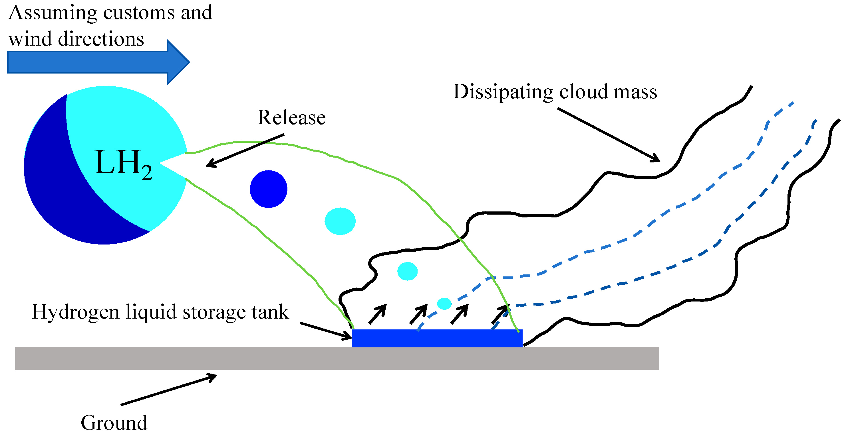
Figure 1: LH2 leakage and dispersion process.
2.2 LH2 Leakage and Liquid-Pool Source-Term Model
At present, source strength is usually calculated based on the liquid-pool size and evaporation rate after leakage, but delayed phase change and related phenomena are not fully considered. In CFD simulations, the atmospheric boundary layer is usually implemented through specific boundary conditions to reproduce dynamic liquid-pool expansion and subsequent evaporation when coupled with an integral model [32]. The leakage and dispersion modules are used to analyze and calculate material release, evaporation, and dispersion, covering various leakage scenarios, including the formation and expansion of an LH2 liquid pool.
When LH2 is released through a rupture opening, the leakage mass flow rate can be expressed as:
After leaking onto the ground, LH2 forms a cryogenic liquid pool. Assuming that the liquid pool spreads approximately in a circular shape on the ground, the mass conservation equation of the liquid pool can be expressed as:
The evaporation of the liquid pool is jointly determined by heat conduction from the ground, convective heat transfer from the air, and environmental radiation. The evaporation mass flow rate is expressed as:
In the CFD model, the hydrogen generated by liquid-pool evaporation is treated as a time-varying velocity inlet, and the inlet velocity is expressed as:
2.3 Governing Equations and Dispersion Model for a Semi-Open Space with Obstacles
Computational fluid dynamics was used to simulate the dispersion behavior of H2 in the station area. The gas-phase flow is governed by the conservation equations of mass, momentum, and energy, while the mixing and diffusion of H2 and air are described by the species transport equation. Because the hydrogen cloud generated after leakage is affected simultaneously by buoyancy, natural wind, and station structures, its dispersion process involves turbulent mixing and local recirculation. Therefore, the Realizable k-ε model was adopted for turbulence closure in this study. Compared with the standard k-ε model, this model is more suitable for predicting complex shear flows, obstacle-induced flow fields, and recirculation regions, and can describe the migration, dilution, and local retention of H2 clouds in semi-open station spaces [33]. The governing equation is as follows:
Continuity Equation:
The momentum equation is:
The energy equation is:
The species transport equation is:
The density of the gas mixture is calculated using the ideal-gas equation of state:
The transport equations for turbulent kinetic energy k and turbulent dissipation rate ε are expressed as:
During ignition and combustion of the hydrogen cloud, the combustion process was simulated using the partially premixed combustion model in ANSYS Fluent. For the station ignition case, the H2 concentration, temperature, and velocity fields obtained from the dispersion simulation at t = 3.0 s are used as the initial flow-field conditions for the combustion calculation, and the leakage-based time coordinate is retained without resetting after ignition. The partially premixed model describes the flame evolution based on the mixture fraction and reaction progress variable, while the chemical reaction process is represented using a detailed H2-air kinetic mechanism consisting of 10 species and 19 elementary reactions. This approach enables the prediction of flame propagation and thermal hazard distribution following ignition of the hydrogen-air cloud.
The overall hydrogen combustion reaction is:
In the partially premixed combustion model, the flame propagation rate is controlled by the turbulent flame speed ST, which is expressed as:
The heat released by combustion is treated as the chemical-reaction heat source term in the energy equation:
The imported H2 kinetic mechanism is used to determine the composition-dependent combustion properties required by the partially premixed formulation, including the laminar flame characteristics used in the turbulent flame-speed closure.
The numerical simulations of LH2 evaporation and dispersion were performed using ANSYS Fluent. A three-dimensional transient pressure-based solver was adopted to capture the temporal evolution of hydrogen dispersion after LH2 leakage. The species transport model was applied to describe the mixing and diffusion process between hydrogen and air, while the turbulence effect induced by buoyancy, natural ventilation, and structural obstacles was modeled using the standard k-ε turbulence model [34]. The pressure–velocity coupling was achieved using the Semi-Implicit Method for Pressure-Linked Equations (SIMPLE) algorithm [35]. The momentum, energy, species transport, and turbulence equations were discretized using the second-order upwind scheme, while pressure interpolation was performed using the second-order scheme. The transient terms were discretized using the second-order implicit scheme. The time-step size was determined based on the characteristic flow velocity, mesh resolution, and numerical stability. The Courant number and residual convergence were monitored during the calculation, and a time-step sensitivity analysis was conducted to ensure the reliability of transient results.
Fluent provides several radiation models, including DTRM, P-1, Rosseland, S2S, and DO, which can account for wall heating or cooling caused by radiation. Among them, the DTRM model has a relatively simple form, and increasing the number of rays can improve calculation accuracy. The P-1 model is suitable for combustion problems with large optical thickness. The Rosseland model has high computational efficiency and low memory demand. The S2S model is mainly used for surface radiative heat transfer in enclosed spaces without participating media. The DO model has a broad range of applicability and can handle radiation problems under different optical thicknesses [36]. Therefore, the DO radiation model is used in this study to predict the influence of radiative heat transfer.
To systematically evaluate the influence of source-term variation after LH2 leakage on the H2 dispersion scenario, this study uses an integral model to simulate liquid-pool expansion and subsequent evaporation after LH2 is released onto the ground. The liquid-pool radius R(t) and mass flow rate m(t) calculated by the integral model are then converted into transient inlet boundary conditions in the CFD model. The time coordinate shown in Fig. 2 is used as the time reference for the dispersion stage. It should be noted that the liquid-pool radius and mass flow rate in Fig. 2 are both close to 0 during t = 0–2.8 s, indicating that no effective liquid-pool source term has formed during this stage. From t ≈ 2.8 s, the mass flow rate and liquid-pool radius begin to increase significantly, indicating that LH2 enters the stage of ground-pool formation and evaporative release.
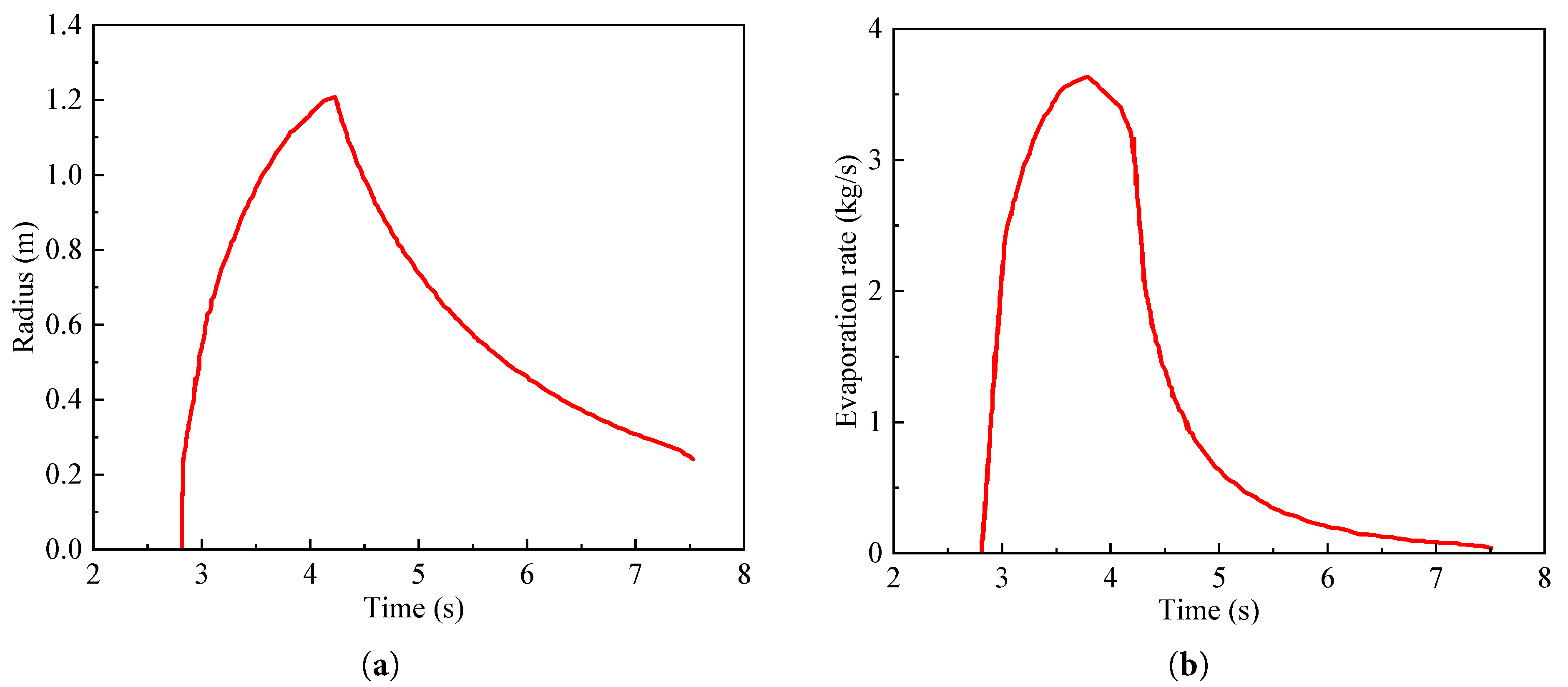
Figure 2: Time variation of evaporation rate and radius of the H2 pool source term (a) The radius changes over time; (b) Evaporation rate varies with time.
After leakage, LH2 is released onto the ground and forms a circular cryogenic liquid pool whose radius varies with time. Bund constraints are not considered in the calculation. Because the temperature of LH2 is much lower than the ambient temperature, continuous heat exchange occurs between the liquid pool and the ground, air, and surrounding solid walls. Liquid hydrogen therefore evaporates continuously and forms an H2 cloud. As shown in Fig. 2, the LH2 source-term evolution has clear unsteady characteristics. During t ≈ 2.8–3.7 s, the liquid pool expands rapidly and the mass flow rate increases quickly. At t ≈ 3.7–3.8 s, the mass flow rate reaches its peak, approximately 3.6 kg/s, indicating that the mass of H2 released into the gas phase per unit time is the largest. The mass flow rate then decreases, while the liquid-pool radius continues to increase and reaches its maximum value of about 1.2 m at t ≈ 4.2 s. This indicates that the maximum liquid-pool expansion lags behind the peak mass flow rate.
After t ≈ 4.2 s, liquid supply weakens and evaporation consumption gradually becomes dominant. The liquid-pool radius begins to shrink, and the evaporation mass flow rate decays rapidly. By t ≈ 7.5–7.6 s, the evaporation mass flow rate has decreased to a negligible level, indicating that the active evaporation source has become very weak. A small residual liquid pool may persist for a short period; by approximately t ≈ 8.5 s, the residual pool nearly disappears and the inlet velocity approaches zero, marking the complete cessation of the evaporation source. Thereafter, no new H2 is introduced into the CFD domain, while the existing H2 cloud continues to migrate, dilute, and disperse under the effects of buoyancy, natural wind, and disturbance from station obstacles. Accordingly, the main source-term evolution can be divided into four stages: t = 0–2.8 s, no effective source term; t ≈ 2.8–3.8 s, rapid release and intense evaporation; t ≈ 3.8–4.2 s, decreasing mass flow rate with continued liquid-pool expansion; and t ≈ 4.2–7.6 s, liquid-pool shrinkage and rapid source-term decay, followed by a short residual-pool disappearance period up to approximately 8.5 s.
In the CFD model, H2 generated by liquid-pool evaporation enters the computational domain through a velocity-inlet boundary. Because Fluent cannot easily describe a time-varying liquid-pool boundary directly, a user-defined function (UDF) is used to define the source term obtained from the integral model as:
Thus, the CFD inlet boundary reflects both the change in liquid-pool area and the change in source strength. Specifically, the inlet source term starts at t ≈ 2.8 s, reaches the maximum mass flow rate at t ≈ 3.7–3.8 s, corresponds to the maximum liquid-pool area at t ≈ 4.2 s, and decays to nearly 0 at t ≈ 7.5–7.6 s. This treatment avoids the error caused by assuming a constant liquid-pool radius and more reasonably describes the early strong source release and later source-term decay after LH2 leakage.
3.2 SValidation of the LH2 Leakage Integral Model
To evaluate the predictive capability of the source-term integral model for LH2 release, pool evaporation, and subsequent gaseous hydrogen cloud evolution, publicly reported NASA large-scale LH2 release experimental data were used for comparison, as shown in Fig. 3 [37]. In the experiment, gas samples were collected using sampling bottles, and hydrogen concentrations were also recorded by hydrogen sensors. Test 6 was selected for validation because, under its wind-field conditions, the hydrogen cloud passed through a relatively large number of monitoring locations, providing sufficient concentration-distribution data for assessing the predicted flammable-cloud envelope. The validation focused on the 4 vol% H2 concentration envelope. The experimental results show that, at 20.94 s after LH2 release, the 4 vol% flammable hydrogen cloud reached a height of approximately 20–25 m and a lateral spreading distance of approximately 37–40 m. The integral model predicted a corresponding cloud height of approximately 20–23 m and a lateral spreading distance of approximately 35–38 m. The predicted flammable-cloud height and lateral extent are generally consistent with the experimental observations, indicating that the integral model can capture the main evolution characteristics of the gaseous hydrogen cloud after LH2 evaporation. The remaining discrepancies may be attributed to wind-speed fluctuations during the experiment, simplified environmental boundary conditions in the model, and the limited spatial resolution of the monitoring points. Overall, the comparison supports the use of the source-term integral model for predicting LH2 pool evaporation and the subsequent formation of the hydrogen cloud. Therefore, the transient liquid-pool radius and evaporation mass flow rate obtained from the integral model can be used as CFD inlet boundary conditions for the subsequent LH2 leakage and dispersion simulations in the station.
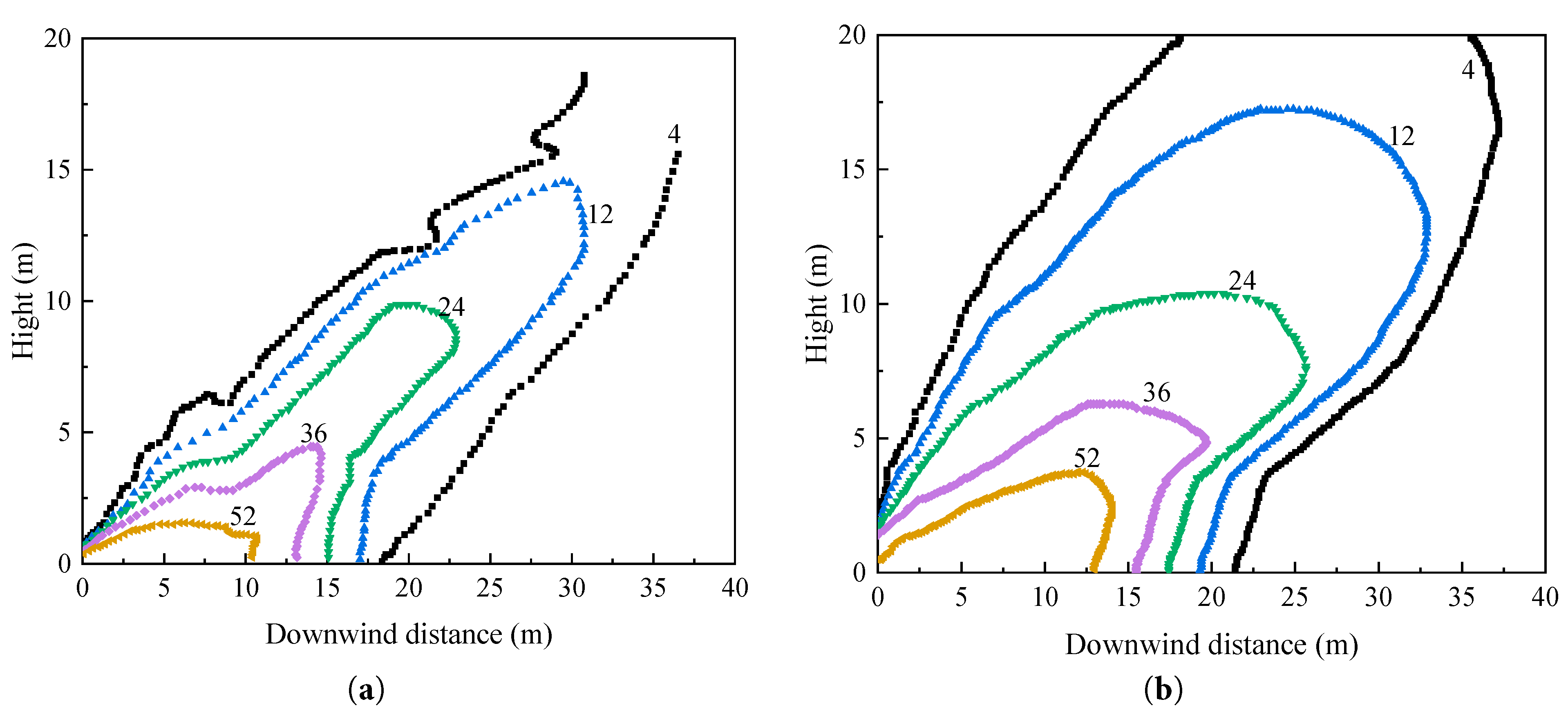
Figure 3: H2 leakage experiment and model verification (a) H2 concentration contour at 20.94 s in the NASA Test 6 experiment; (b) H2 concentration contour obtained from the integral-model simulation.
The layout of the station and its surrounding area can strongly influence hydrogen-cloud dispersion. A simplified geometric model is established based on the main structural features of the station, as shown in Fig. 4. The four sides are open. Natural wind enters from the left side and exits from the other three sides. The inlet wind speed was set to 2 m/s to represent a weak natural-ventilation condition in the semi-open station, consistent with the baseline ventilation condition commonly adopted in locomotive-related hydrogen dispersion simulations [38]. Nine support columns with dimensions of 1 m × 1 m × 6 m are arranged in the station. The locomotive length is 30 m. The center of the LH2 liquid pool is located at the coordinate origin, and the locomotive head is 50 m from the air inlet. The H2 dispersion simulation uses the same source conditions described above. The computational domain is shown in Fig. 4a, and the boundary conditions are listed in Table 2.
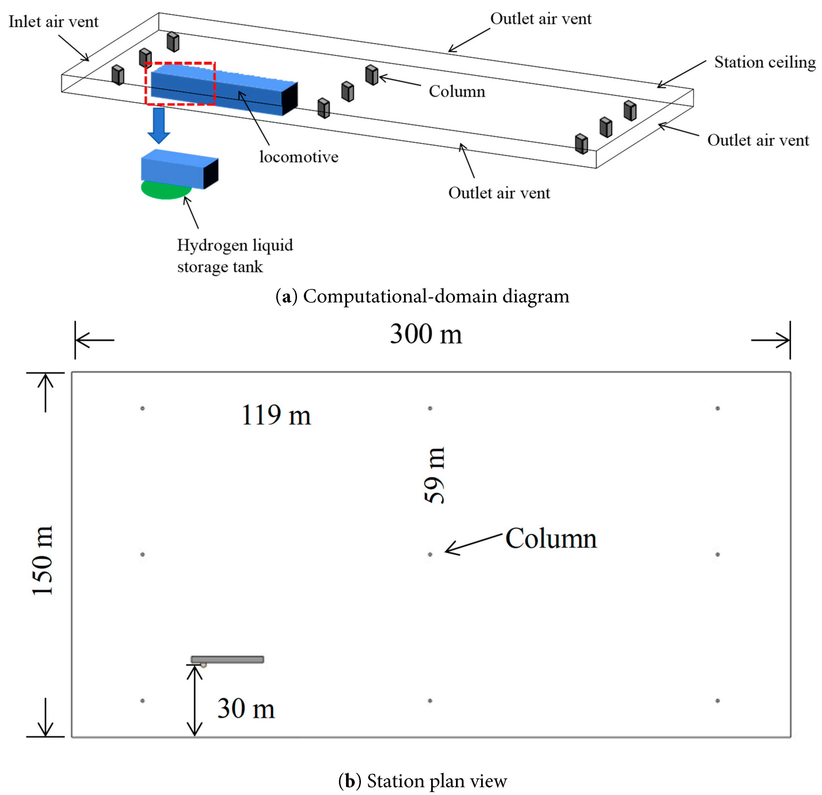
Figure 4: Station structure (a,b).
Table 2: Boundary conditions.
| Parameter | Type | Value setting |
|---|---|---|
| Station air inlet | Velocity inlet | Inlet wind speed: 2 m/s; inlet temperature: 300 K |
| Station air outlet | Outlet-vent | Backflow temperature: 300 K |
| Station roof, ground, support columns, and locomotive walls | Wall | Isothermal wall; wall temperature: 300 K |
| LH2 liquid-pool evaporation source/H2 inlet | Velocity inlet | Velocity inlet; prescribed through a UDF [39]; inlet temperature fixed at the phase-transition temperature of LH2 |
| Combustion calculation boundary | Same as the dispersion-simulation boundary conditions | - |
3.4 Basic Verification of the Species Transport Model
To verify the basic capability of the species transport model, the gas leakage and dispersion experiment conducted by Liu et al. [40] in a gas-cabin pipeline is used as a reference. It should be noted that this case is not dynamically or geometrically similar to the full-scale LH2 leakage and H2 dispersion scenario in the semi-open railway station. Instead, it is used only to examine whether the adopted species transport and turbulence models can capture the basic processes of gas advection, accumulation, and dilution under controlled release conditions. The experiment used non-toxic substitute gases (N2 for fuel gas and CO2 for air) in a rectangular pipe gallery with a cross-section of 85 mm × 170 mm and a length of 10 m. Gas was vertically released from an inlet 25 mm above the ground, with a mass flow rate of 1.587 × 10⁻⁴ kg/s. In the numerical simulation, multiple monitoring points are arranged. The same species transport and turbulence models as those used in the H2 dispersion simulation are adopted. The experimental and simulated results are compared to evaluate the feasibility of the CFD method for predicting gas dispersion.
Fig. 5 compares the experimental and simulated N2 volume fractions at the monitoring point over time. Both the experimental and simulated values show an overall increasing trend with leakage time, indicating that the model can capture gas accumulation and dispersion in confined spaces after release. The simulated values are lower than the experimental values at the early leakage stage, indicating a certain delay in the model response to early local concentration growth. As dispersion develops, the simulated curve gradually approaches the trend of the experimental data. The difference between them may be related to experimental measurement uncertainty, simplification of inlet release conditions, and local turbulent fluctuations. Overall, this comparison indicates that the adopted species transport and turbulence models can reproduce the basic trend of gas accumulation and dilution in a controlled duct experiment. However, because the N2/CO2 case differs from the present LH2 station scenario in release rate, length scale, temperature, and buoyancy behavior, it is used only as a basic verification of gas transport rather than as a direct validation of the full station-scale LH2 dispersion process.
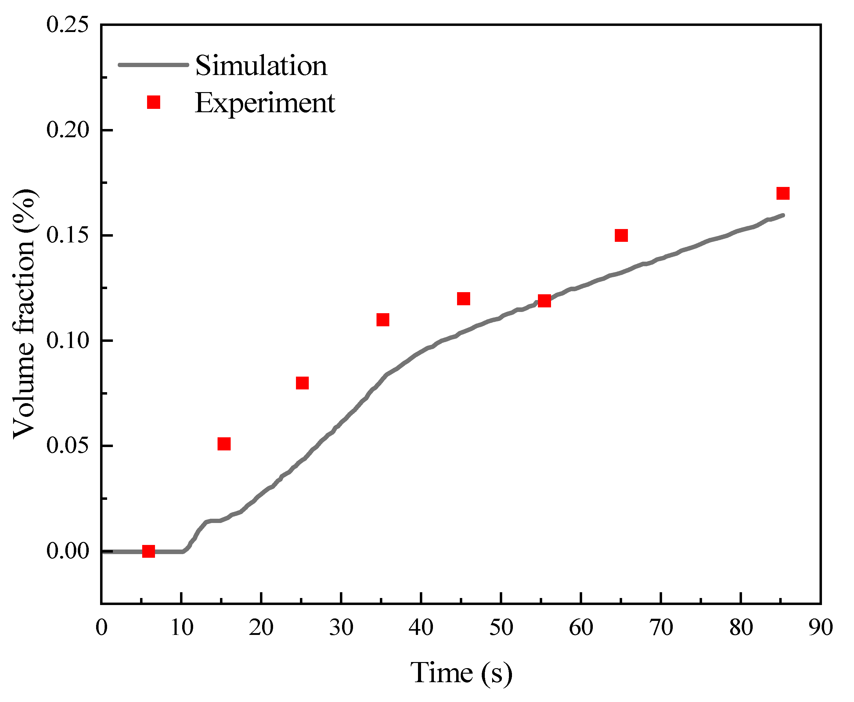
Figure 5: Comparison of experimental and simulated N2 volume fractions.
3.5 Flame Combustion Model after LH2 Evaporation and Dispersion
The H2-air flammable cloud formed during LH2 evaporation and dispersion may burn when exposed to an open flame, high-temperature surface, electric spark, or other ignition source. Because H2 has a wide flammability range and a low minimum ignition energy, local flammable clouds formed during the dispersion stage have high ignition sensitivity. Therefore, after obtaining the H2 concentration and temperature fields in the station space, a combustion calculation model is established to analyze flame propagation and temperature-field evolution after ignition. The combustion calculation inherits the H2-air mixed-cloud distribution obtained from the dispersion stage and sets a local ignition source in the flammable region to trigger combustion. The ignition source is treated as an equivalent high-temperature region. The combustion simulation uses a pressure-based transient solver. The governing equations include mass, momentum, energy, and species transport equations. Turbulence closure uses the Realizable k-ε model. The H2 combustion reaction mechanism is imported through Chemkin and contains 10 species and 19 elementary reactions. The contribution of radiation heat transfer to the flame temperature field and the thermal impact on surrounding walls is also considered. The time step is determined according to flame propagation velocity, mesh size, and convergence stability, and time-step sensitivity checks are performed to ensure the reliability of transient combustion results. To verify the predictive ability of the combustion model for H2-air flame propagation, the H2-air combustion experiment performed by Liu et al. [41] is used for comparison. The experimental device is a cylindrical reaction vessel with an inner diameter of 0.4 m and a height of 2.3 m. The validation calculation establishes a two-dimensional axisymmetric model according to the experimental geometry and initial conditions, and a local ignition source is placed at the same ignition position as in the experiment. In the validation cases, the initial temperature is 373 K and the H2 volume fraction is 8%–12%. The main comparison is the flame-front position over time under different hydrogen concentrations. A small time step is used to capture the rapid propagation of the flame front, and the experimental results are used to evaluate the model prediction of the H2-air flame propagation trend. For the station scenario, the ignition condition is determined from the dispersion-stage concentration field, and a location is treated as ignitable when the local H2 volume fraction is within 4–74 vol%. In the ignition/combustion branch, the t = 3.0 s dispersion field is selected as the ignition initial field, and ignition is imposed at (−0.7, −3.6, 0.5) m. The same time coordinate measured from the onset of LH2 leakage is retained throughout the combustion calculation and is not reset after ignition.
Fig. 6 compares the experimental and simulated flame-front positions under different H2 volume fractions. The results show that when the H2 volume fraction is 10% and 12%, the simulation can reproduce the trend of flame-front propagation over time. When the H2 volume fraction is 6%, there is a certain deviation between the simulated and experimental results, but the overall increasing trend of the flame-front position remains basically consistent. The deviation may arise from simplification of the ignition process, the two-dimensional axisymmetric model approximation, uncertainty in the turbulent combustion model, and experimental measurement errors. Overall, the validation results show that the detailed H2 reaction mechanism and turbulent combustion model used here can reasonably describe flame propagation after ignition of an H2-air mixture and can be used for engineering-scale analysis of combustion consequences in the station scenario.
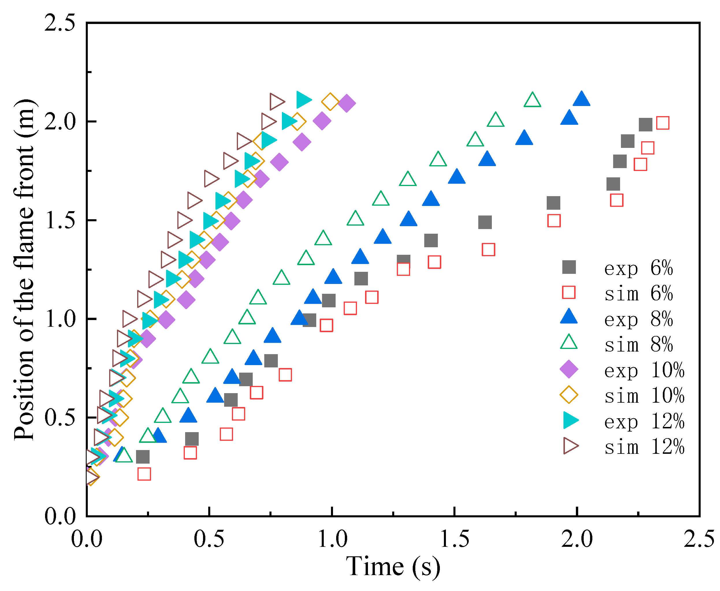
Figure 6: Comparison of experimental and simulated flame-front positions.
3.6 Grid-Independence Verification
To ensure the accuracy of the numerical results while maintaining reasonable computational efficiency, five mesh models containing 4.8 × 10⁵, 5.0 × 10⁵, 5.8 × 10⁵, 6.4 × 10⁵, and 7.1 × 10⁵ cells were generated. Considering the influence of the support columns on the local flow field and hydrogen dispersion, local mesh refinement was applied in the vicinity of the columns to improve the resolution of the flow-field variations around these obstacles, as illustrated in Fig. 7a. Grid sensitivity was evaluated for both the dispersion and combustion stages. For the dispersion stage, the time-varying H2 volume fraction at the monitoring point (0, 0, 6) was selected as the evaluation parameter. For the combustion stage, the temperature distribution along a 30-m-long monitoring line oriented in the Y direction at a height of 1.6 m was compared under different mesh resolutions. As shown in Fig. 7b, differences in the transient H2 volume fraction at (0, 0, 6) decrease progressively with increasing mesh density. When the number of cells increases from 5.8 × 10⁵ to 6.4 × 10⁵ and 7.1 × 10⁵, only minor differences are observed among the concentration curves. A similar tendency is observed for the combustion calculation, as shown in Fig. 7c, where the temperature distributions along the monitoring line obtained using the three finer meshes are in close agreement. Further mesh refinement therefore produces only limited changes in both the predicted H2 dispersion and temperature distribution. Considering the balance between numerical accuracy and computational cost, the mesh containing 5.8 × 10⁵ cells was selected for the subsequent dispersion and combustion simulations.
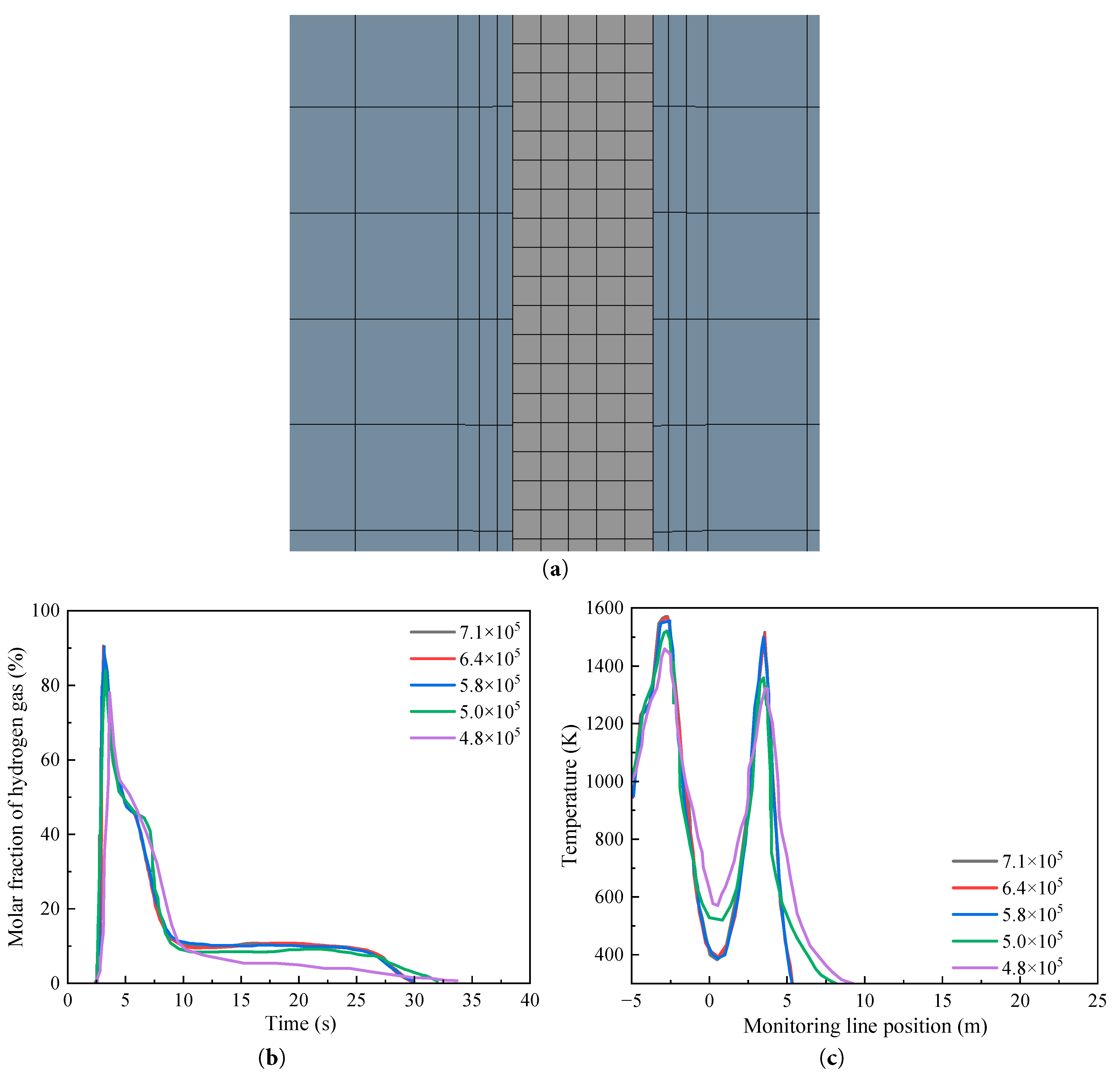
Figure 7: Grid-independence verification (a) Section mesh at the column sectionv; (b) H2 volume fraction at the monitoring point; (c) Temperature distribution along the Y-direction monitoring line.
4.1 LH2 Evaporation and Dispersion in the Station
Fig. 8 shows the H2 distribution formed in the vertical mid-plane of the station and above the liquid pool after LH2 evaporation. After being released onto the ground, LH2 first undergoes liquid outflow, ground spreading, and heat-induced evaporation. A clear gas-phase H2 evaporation source term forms after approximately 2.8 s. Low-temperature H2 then forms a high-concentration region above the liquid pool and disperses upward and downwind under the combined effects of buoyancy and lateral wind. During t = 7.6–8.0 s, the already weak evaporation source continues to decay and the residual pool boundary shrinks. At about t = 8.5 s, the residual liquid pool nearly disappears and the inlet velocity approaches zero, marking the complete cessation of the evaporation source. Afterward, no new H2 is introduced into the computational domain. The existing H2 cloud continues to migrate and dilute under buoyancy, natural wind, and station-structure disturbances. This process shows that the early hazard after LH2 leakage is not instantaneous. Instead, it is a dynamic process jointly controlled by liquid-pool spreading, evaporation enhancement, and source-term decay. Fig. 8 shows the H2 distribution formed in the vertical mid-plane of the station and above the liquid pool after LH2 evaporation. After being released onto the ground, LH2 first undergoes liquid outflow, ground spreading, and heat-induced evaporation. A clear gas-phase H2 evaporation source term forms after approximately 2.8 s. Low-temperature H2 then forms a high-concentration region above the liquid pool and disperses upward and downwind under the combined effects of buoyancy and lateral wind. During t = 7.6–8.0 s, the already weak evaporation source continues to decay and the residual pool boundary shrinks. At about t = 8.5 s, the residual liquid pool nearly disappears and the inlet velocity approaches zero, marking the complete cessation of the evaporation source. Afterward, no new H2 is introduced into the computational domain. The existing H2 cloud continues to migrate and dilute under buoyancy, natural wind, and station-structure disturbances. This process shows that the early hazard after LH2 leakage is not instantaneous. Instead, it is a dynamic process jointly controlled by liquid-pool spreading, evaporation enhancement, and source-term decay.
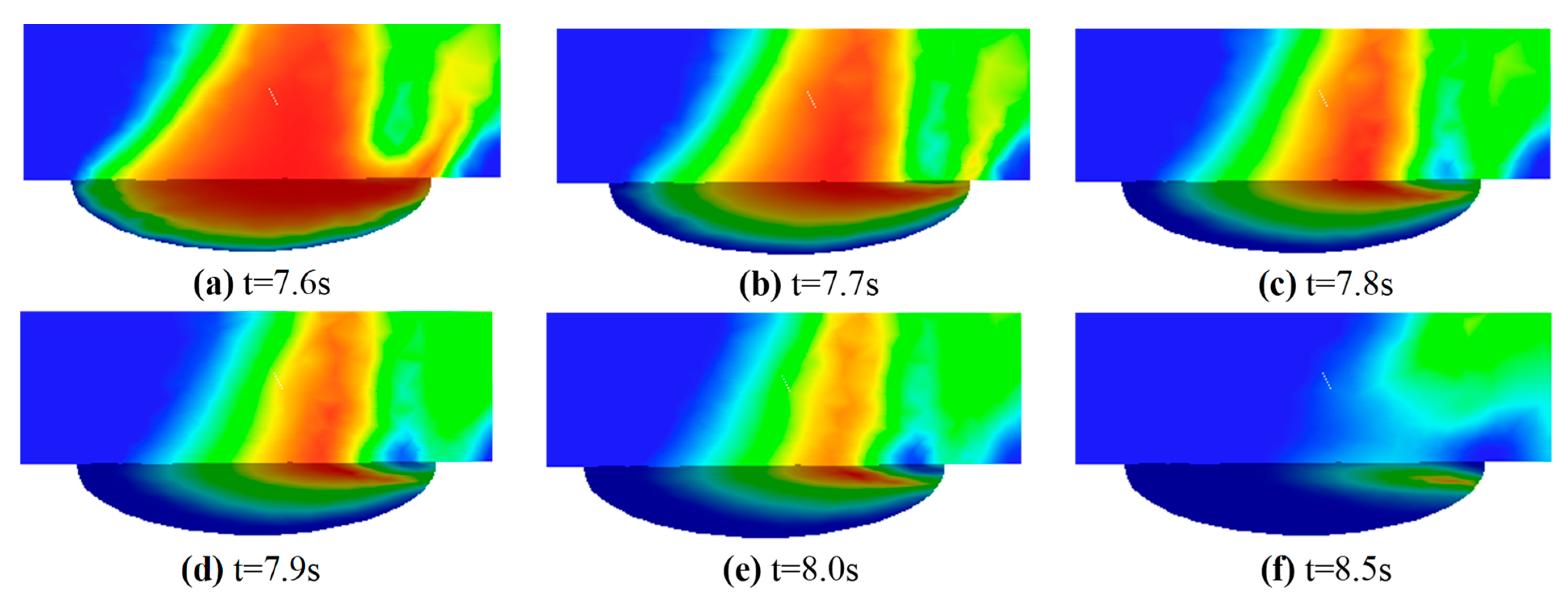
Figure 8: H2 volume-fraction distribution in the vertical mid-plane and above the pool (a–f).
Fig. 9 shows the time evolution of the front position and length of the H2 dispersion cloud in the station. The results indicate that at 4 s after LH2 leakage, the H2 cloud front has advanced 2.81 m compared with that at 3 s, and the cloud length reaches 10.06 m. The changes in front displacement and cloud length at this stage may be related to wind-speed conditions and the station computational-domain layout. At t = 5 s, the H2 cloud front is located at 9.25 m, and the cloud length is 16.48 m, increasing by approximately 2 m compared with the previous 2 s. This indicates a relatively high dispersion rate at this time. By 9 s, the cloud front has advanced to 22.42 m, and the cloud length has increased to 28.92 m. As dispersion continues, the H2 cloud gradually separates from the ground and further expands outward in the upper region of the station. To analyze H2 dispersion more intuitively, the velocity distribution of the 4% H2 volume-fraction iso-surface at 9 s after leakage is further presented.
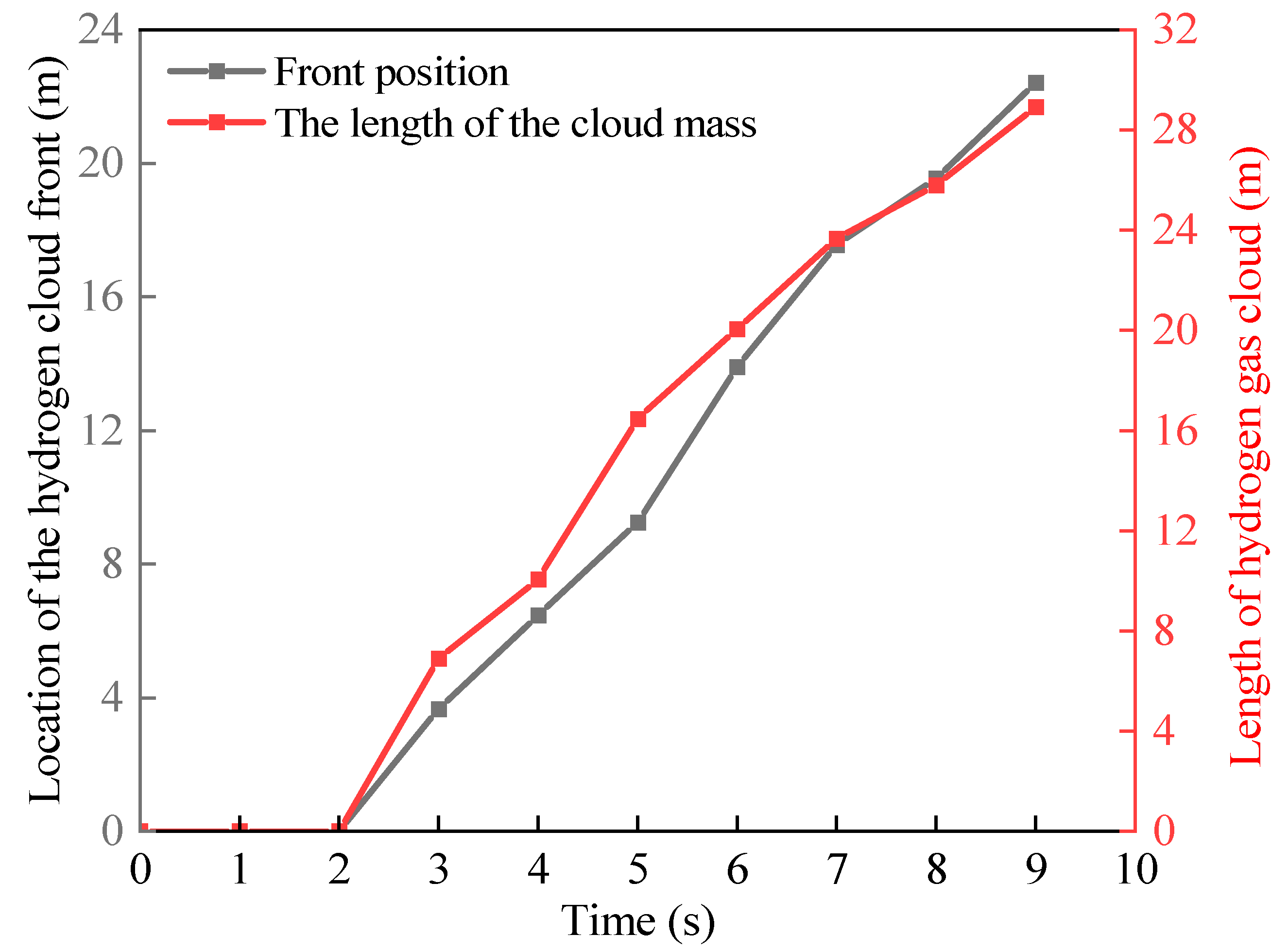
Figure 9: Time history of cloud-front position and cloud length.
Fig. 10 shows the velocity distribution of the 4% H2 volume-fraction iso-surface in the station at 9 s after leakage, including front, side, and top views. The results show that the H2 cloud has almost surrounded the locomotive, and the H2 concentration around the locomotive is relatively high. Under buoyancy, most H2 migrates toward the station roof and disperses along the roof. The maximum cloud velocity at this time is 3.11 m/s, while the cloud velocity in some regions near the roof is relatively low. The top view indicates that the dispersion footprint of the H2 cloud is large and has covered the area around the locomotive, which may affect locomotive safety. As dispersion continues, the H2 cloud is expected to continue migrating under the wind field and further expand along the station roof. This t = 9 s result belongs to the non-ignited dispersion branch and is used only to characterize the spatial extent and migration of the flammable H2 cloud. It is not used as the initial field for the combustion calculation. At this time, the locomotive is already located within the lower-flammability envelope of the H2 cloud, indicating a substantial dispersion hazard if ignition does not occur earlier.
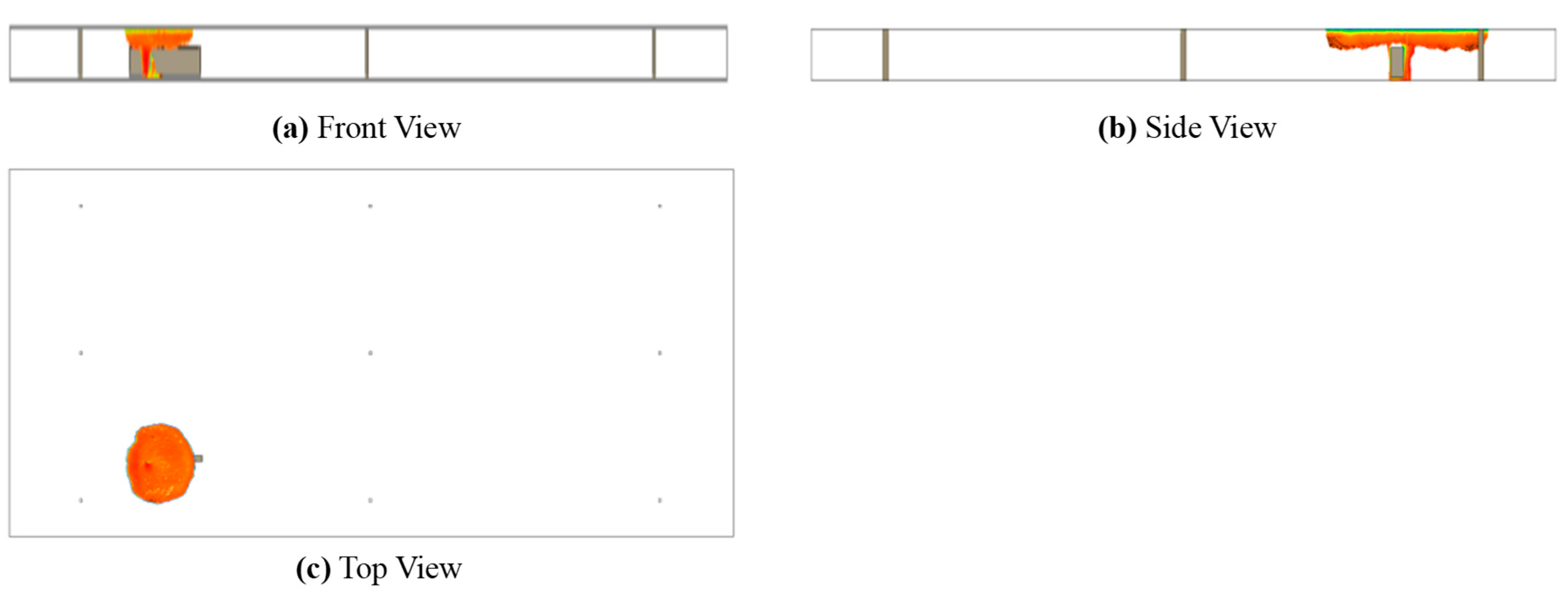
Figure 10: Velocity diagram of the station iso-surface at 9 s (gas concentration: 4%) (a–c).
Fig. 11 shows the H2 concentration distribution on the Z = 6 m plane at five time points in the late dispersion stage. After the leakage release stops, the flammable H2 cloud continues to disperse around the station and reaches a certain limiting dispersion range between the source position and the roof. Its overall position remains relatively stable. As the dispersion range of the H2 cloud continuously expands, the internal concentration gradually decreases until the cloud completely dissipates. The dissipation process lasts approximately 200 s. Therefore, the H2 concentration distributions at 40 s, 80 s, 120 s, 160 s, and 200 s are selected for comparison, and the influence of support columns on H2 cloud dispersion is analyzed. At 40 s, the H2 cloud is further diluted compared with the earlier stage, and the concentration decreases significantly, with a maximum volume fraction of 0.056. At 80 s, the cloud volume continues to increase, and air entrainment is enhanced. Due to obstruction by support columns, the dispersion speed in the downwind direction around the columns decreases, and the maximum volume fraction drops to 0.0184. At 120 s, the cloud area continues to expand outward, but the increase in volume is smaller than in the earlier stage. At 160 s and 200 s, the dispersion area of the H2 cloud changes only slightly, indicating that it gradually enters a passive dispersion stage. Due to vortices on the leeward side of support columns, the local H2 concentration decreases rapidly and the flow velocity is low, indicating that support columns have a certain influence on H2 dispersion.
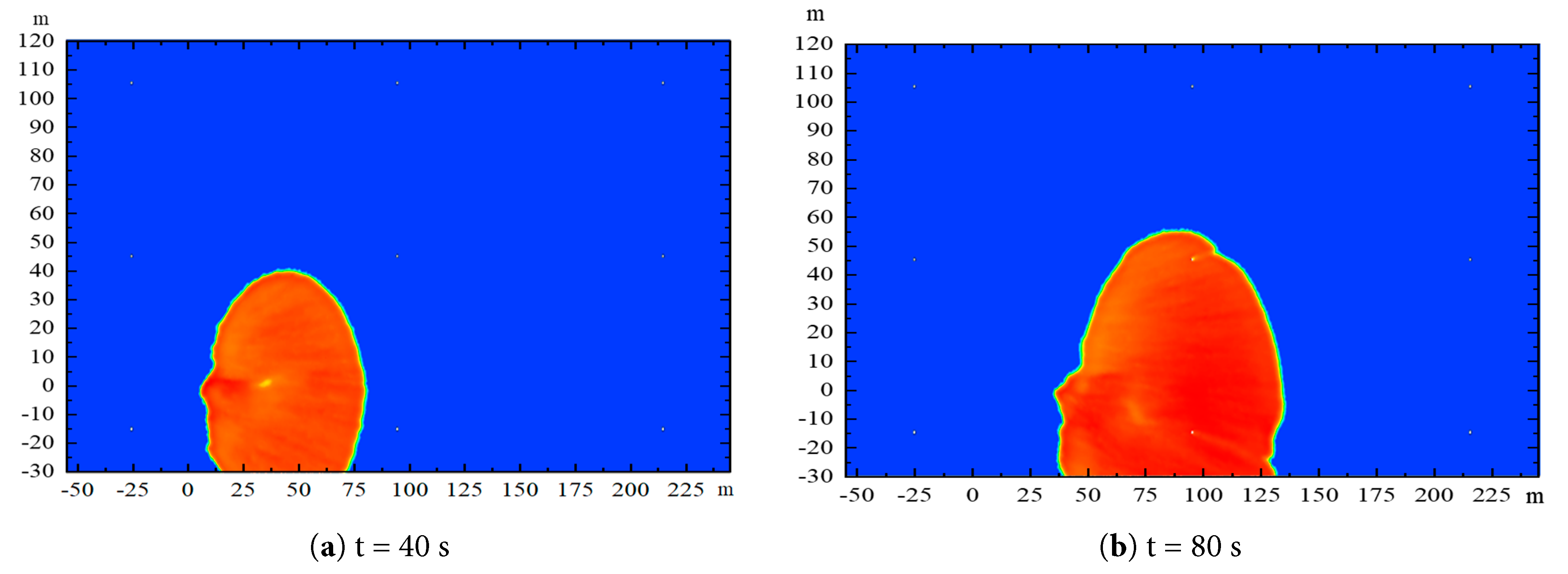
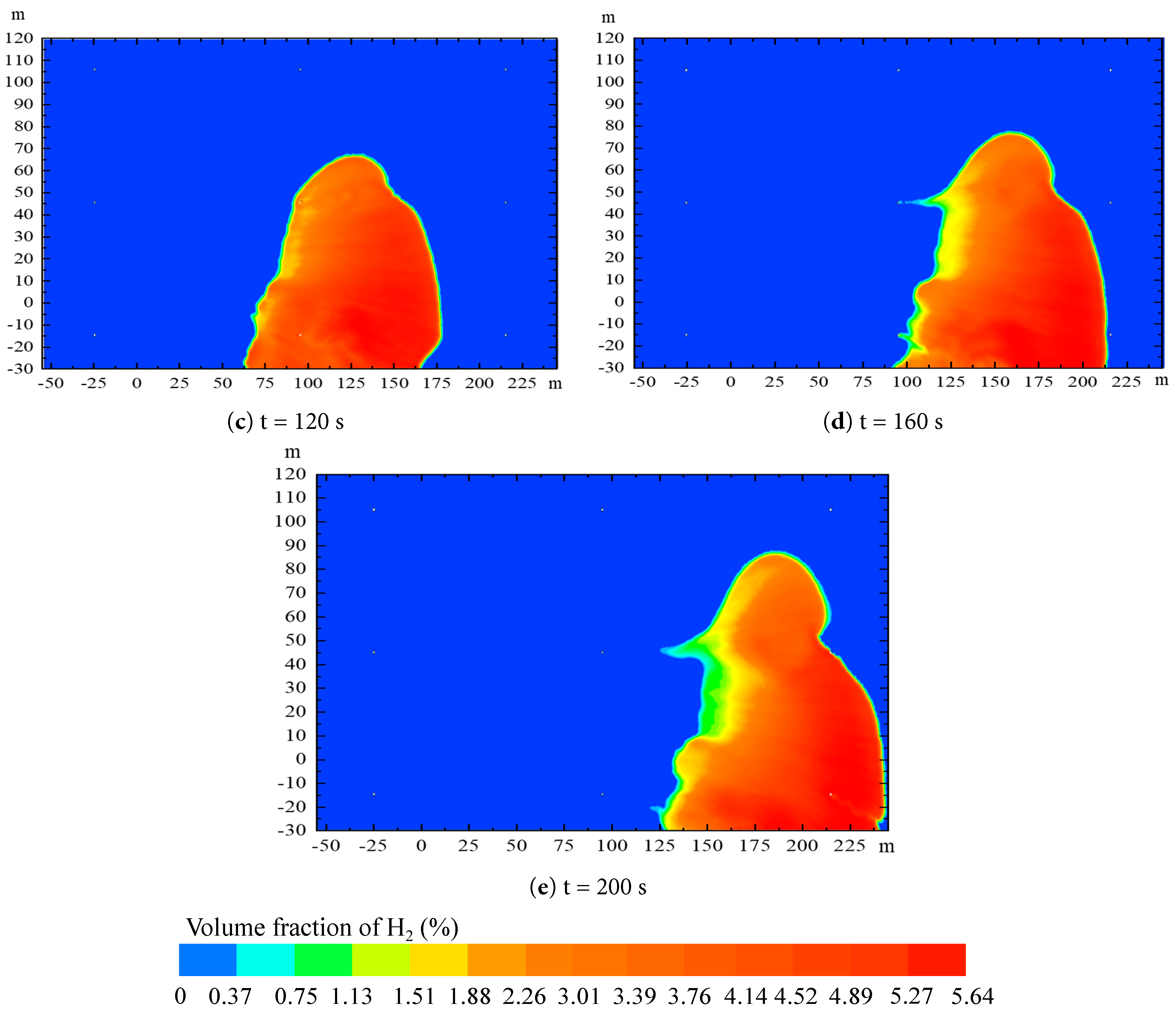
Figure 11: Schematic diagram of H2 cloud concentration variation in the late dispersion stage (a–e).
Fig. 12 shows the monitoring-point arrangement and the variation in H2 percentage. C7 is located directly above the LH2 liquid pool at (0, 0, 6). Its H2 concentration reaches 0.9 at 4 s and then gradually decreases to 0 at around 31 s. C8 is close to the inlet and is 10 m from the LH2 liquid pool. Its monitored concentration remains 0, indicating that H2 mainly disperses along the station roof and downwind. C9 is located at (0, 10, 6), and its H2 concentration reaches a peak value of 0.405 at 5.6 s, indicating local accumulation in this region during the early dispersion stage. C10 and C11 are located 10 m in the positive and negative X directions, respectively, with a Y coordinate of 0 and a height of 6 m. The results show that the H2 concentration at the monitoring point in the negative X direction is higher than that in the positive X direction, whereas the positive X direction detects H2 concentration changes earlier. This may be related to the blocking effect of the locomotive on dispersion in the negative X direction.
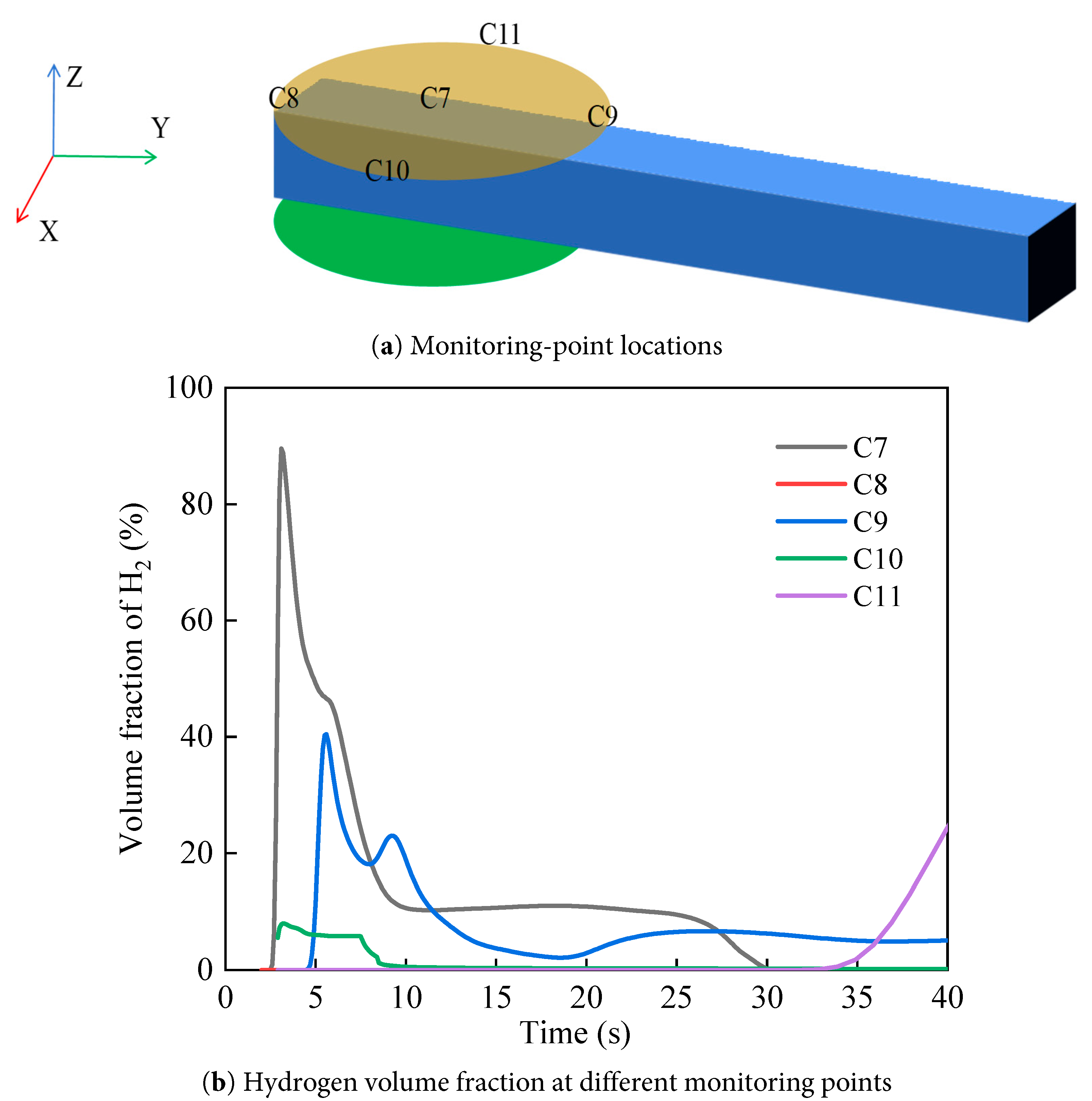
Figure 12: Monitoring-point locations and results (a,b).
4.2 H2 Combustion Distribution in the Station
As shown in Fig. 13a, a monitoring line in the Y direction is placed beside the locomotive to evaluate flame combustion characteristics around the locomotive and personnel safety risk during the fire. The monitoring line is located at X = 0, with a total length of 30 m and a height of 1.6 m. Fig. 13b shows the temperature measured along the Y line over time. The results show that at 4 s, the flame has reached the front edge of the locomotive, and the local temperature can reach 979 K. At Y = 8.4 m, the temperature is about 300 K, indicating that the region within Y = 8.4 m is affected by high temperature at this time. The temperature peak appears at Y = −2.55 m, and this distribution may be related to the station spatial structure and wind-speed conditions. At 5 s, the average flame temperature decreases, and the maximum temperature is 849.6 K, which is 128.9 K lower than the peak temperature at 4 s. Nevertheless, it may still threaten personnel safety and equipment integrity. At 10 s, local high-temperature regions still exist near the Y line. By 15 s and 20 s, the temperature fluctuation along the Y line has weakened significantly and gradually returns to near ambient temperature. These results provide a reference for personnel safety assessment and protective-measure development during the early stage of a fire.
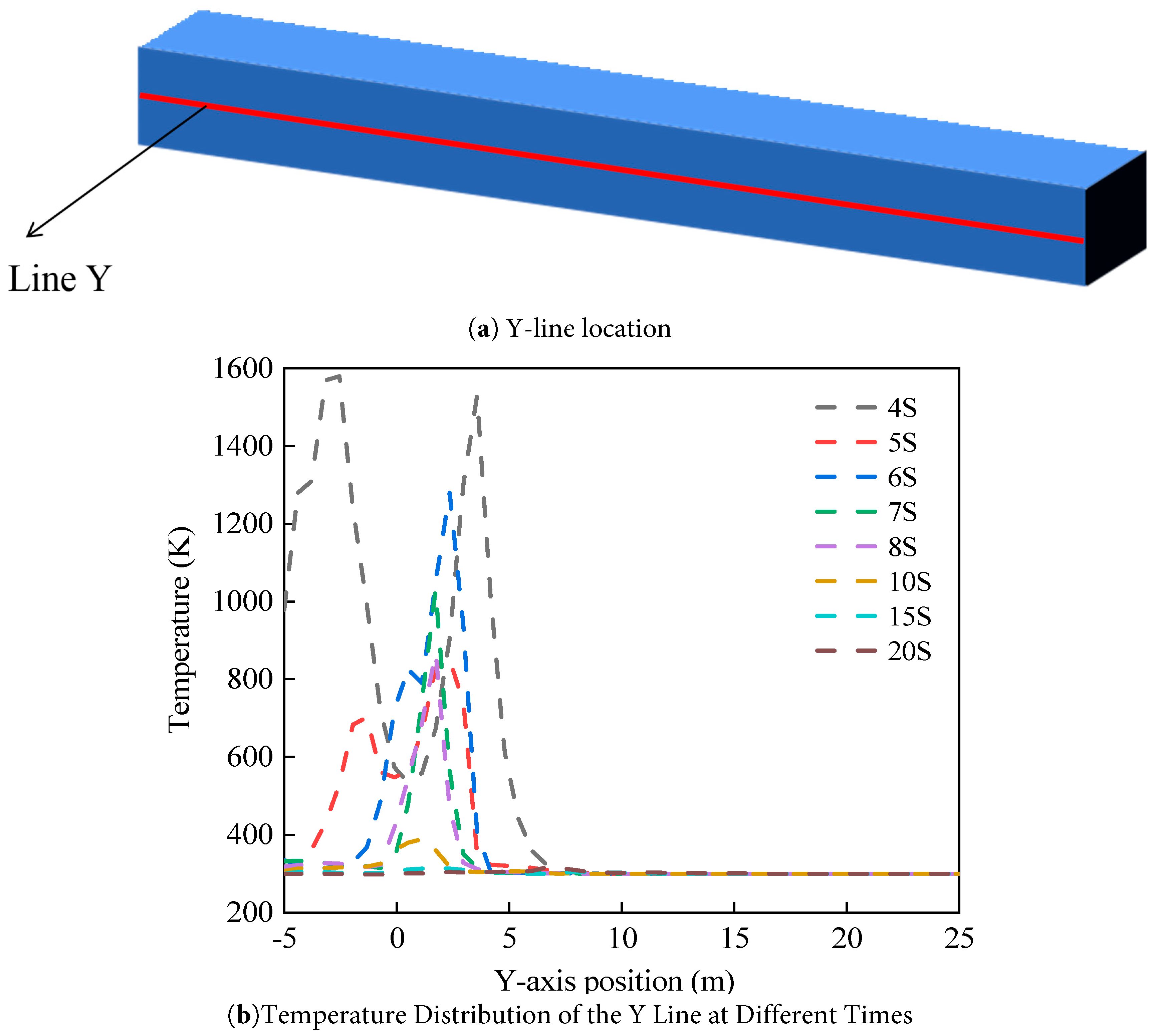
Figure 13: Y-line location and temperature variation (a,b).
A single monitoring dataset is insufficient for comprehensive assessment of accident hazards. Therefore, this study further analyzes the temperature variation over time at different heights in the direction perpendicular to the locomotive. After a fire occurs, personnel may evacuate from the area around or near the middle of the locomotive. To evaluate the thermal hazard in this region, a Z-direction monitoring line with a height of 6 m is arranged at X = 0 m and Y = 10 m, using the coordinate origin as the reference. Fig. 14a shows the position of the Z line in the station physical model. The temperature distribution at different heights along the Z line during the fire can provide a basis for personnel safety-risk assessment. Fig. 14b shows the temperature distribution along the Z line at different time periods. Unlike the Y-line monitoring results, the Z-line temperature at 4 s is close to ambient temperature, indicating that the flame has not yet propagated to this position. At t = 5 s, the temperature begins to rise at heights of 2 m and above from the ground, and the top temperature reaches the maximum value of 1882.3 K. This indicates that the flame propagates around the locomotive with a certain inclination angle. The temperature at a height of 1.6 m is about 300 K, indicating a weak thermal impact at this height. At 8 s, the flame-temperature peak is about 183 K higher than those at 6 s and 7 s, and the peak position changes. At 15 s and 20 s, the temperature in this region has decreased to near ambient temperature, indicating that most of the flame has moved away from this position and that the thermal hazard has decreased significantly. These results provide a reference for personnel evacuation and emergency response during fire accidents.
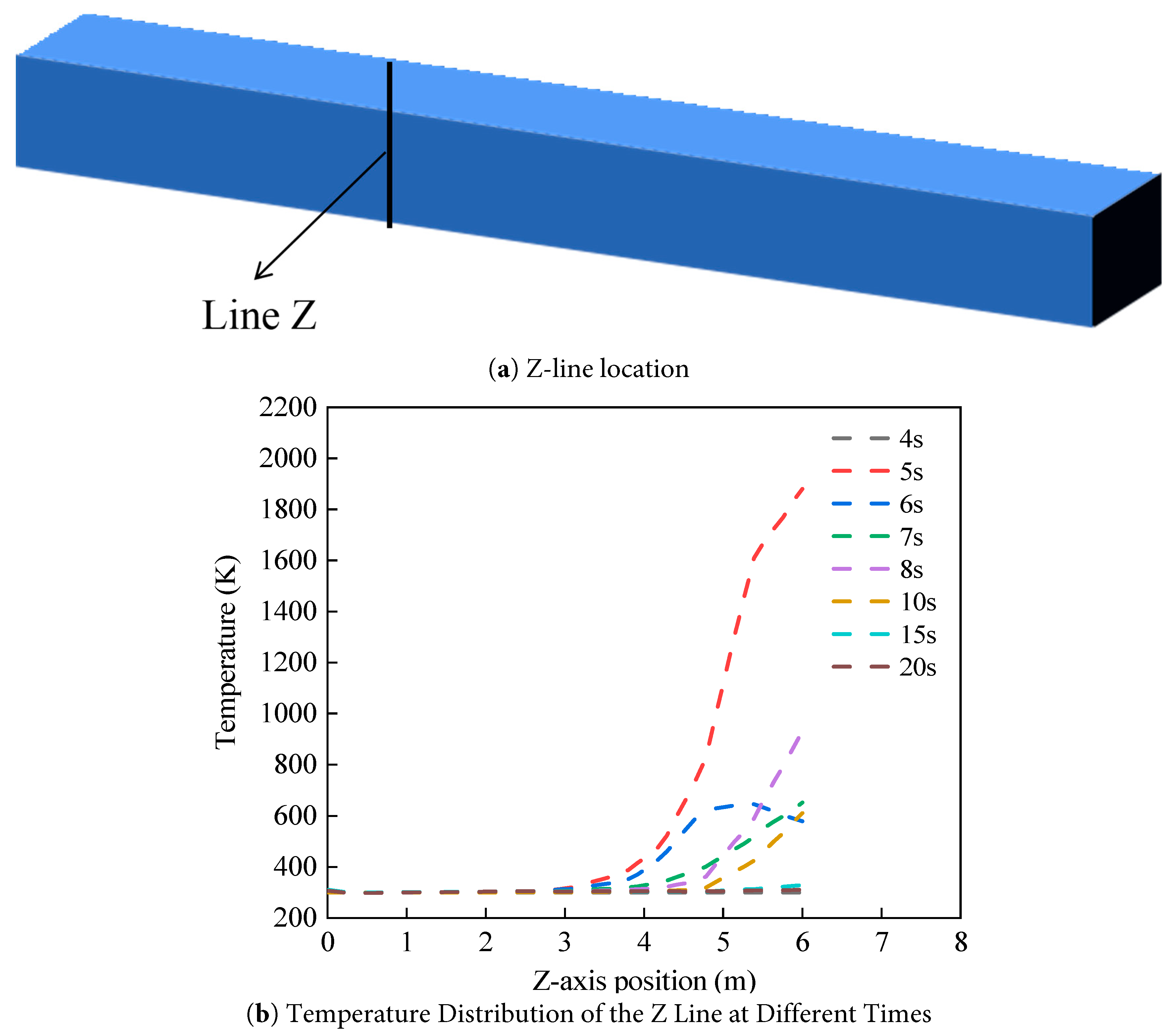
Figure 14: Variation in Z-line values and temperature at different times (a,b).
Fig. 15 shows the time variation of turbulent kinetic energy and temperature at a specific point on the station roof. The monitoring point is located at (0, 10, 6), and it is used to analyze the transient variations in local temperature and turbulent kinetic energy during flame combustion. The results show that at t = 5 s, the turbulent kinetic energy at this point reaches a peak of 2.14 J/kg, and the corresponding temperature is 1882.3 K, consistent with the Z-line monitoring results. Subsequently, both turbulent kinetic energy and temperature gradually decrease with time. The minimum turbulent kinetic energy is 0.0156 J/kg, corresponding to a temperature of 310.9 K. Because the station space is relatively open, flame propagation is weakly constrained except by the locomotive, roof, and support columns. The flammable H2 cloud mainly undergoes jet combustion along the roof. Therefore, flame propagation is less confined, and local turbulent kinetic energy and temperature decay rapidly. At 40 s, the turbulent kinetic energy is 0.03 J/kg and the temperature is 346.8 K, indicating that this point is still affected by heat to some extent, possibly due to radiative heat transfer and residual heat diffusion.
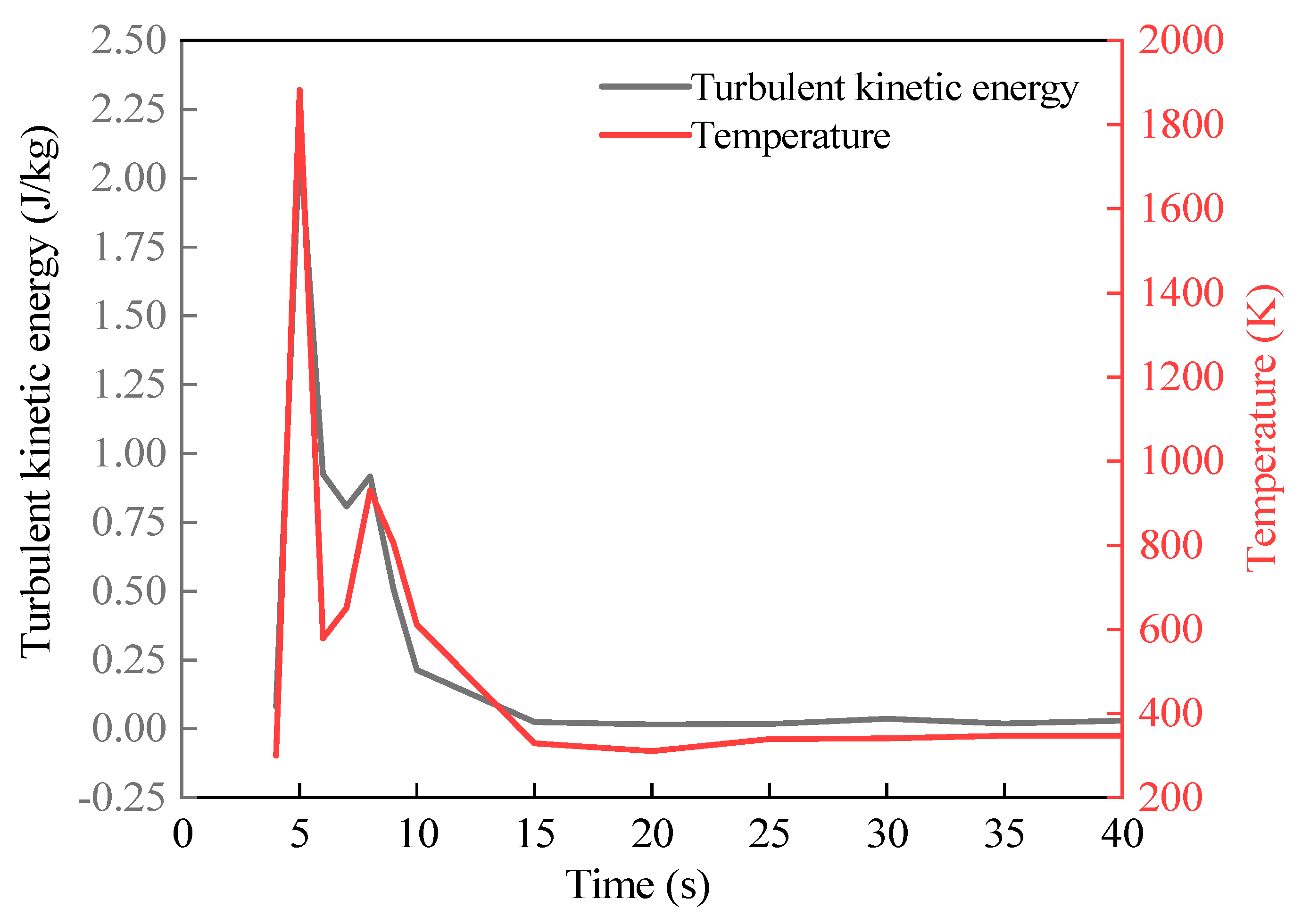
Figure 15: Relationship between turbulent kinetic energy and temperature over time.
Fig. 16 shows the peak flame temperature at different times during the station accident, which is used to analyze the maximum temperature that may be reached in the station area during fire development. The high temperature generated by the fire poses a significant threat to personnel safety and surrounding facilities. Therefore, determining the peak temperature at different times is important for risk assessment. The results show that the highest temperature in the station during the entire combustion process is 2193.5 K, appearing at t = 3.5 s at the location (−0.7, −3.6, 0.574). This indicates that the region beneath the locomotive is one of the main high-temperature hazard zones. During the early fire stage of t = 3–7 s, the peak flame temperature remains above 2000 K, indicating that the area around the locomotive remains at a high temperature. At t = 8 s, the highest flame temperature in the station decreases to 1859.87 K. At about t = 40 s, the maximum temperature around the locomotive decreases to 894 K, and the temperature in most regions is close to 300 K.
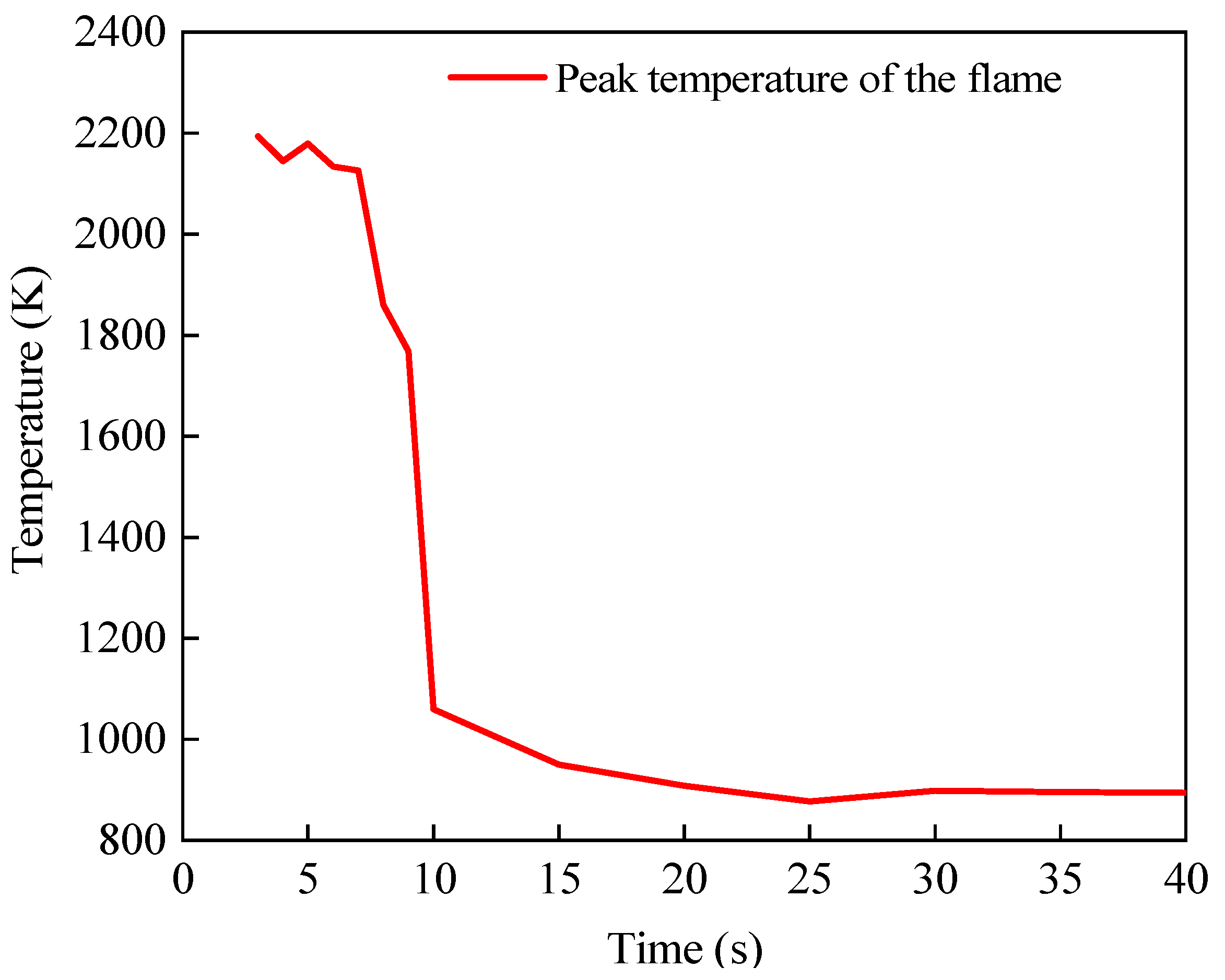
Figure 16: Peak flame temperature at different time periods.
Fig. 17 shows the temperature variation at the monitoring points over time. To analyze the thermal impact in the locomotive-tail region, four temperature monitoring points are arranged at the locomotive tail: D1(−1, 25, 0.35), D2(−1, 25, 1.9), D3(−1, 25, 3.9), and D4(−1, 25, 6). The monitoring results show that the locomotive-tail temperature increases with height. The temperature near the upper region is higher, whereas the near-ground temperature is close to ambient temperature. Among the monitoring points, D4 reaches the highest temperature of 604.7 K at 9.4 s. Overall, the thermal impact on the locomotive-tail region is relatively weak.
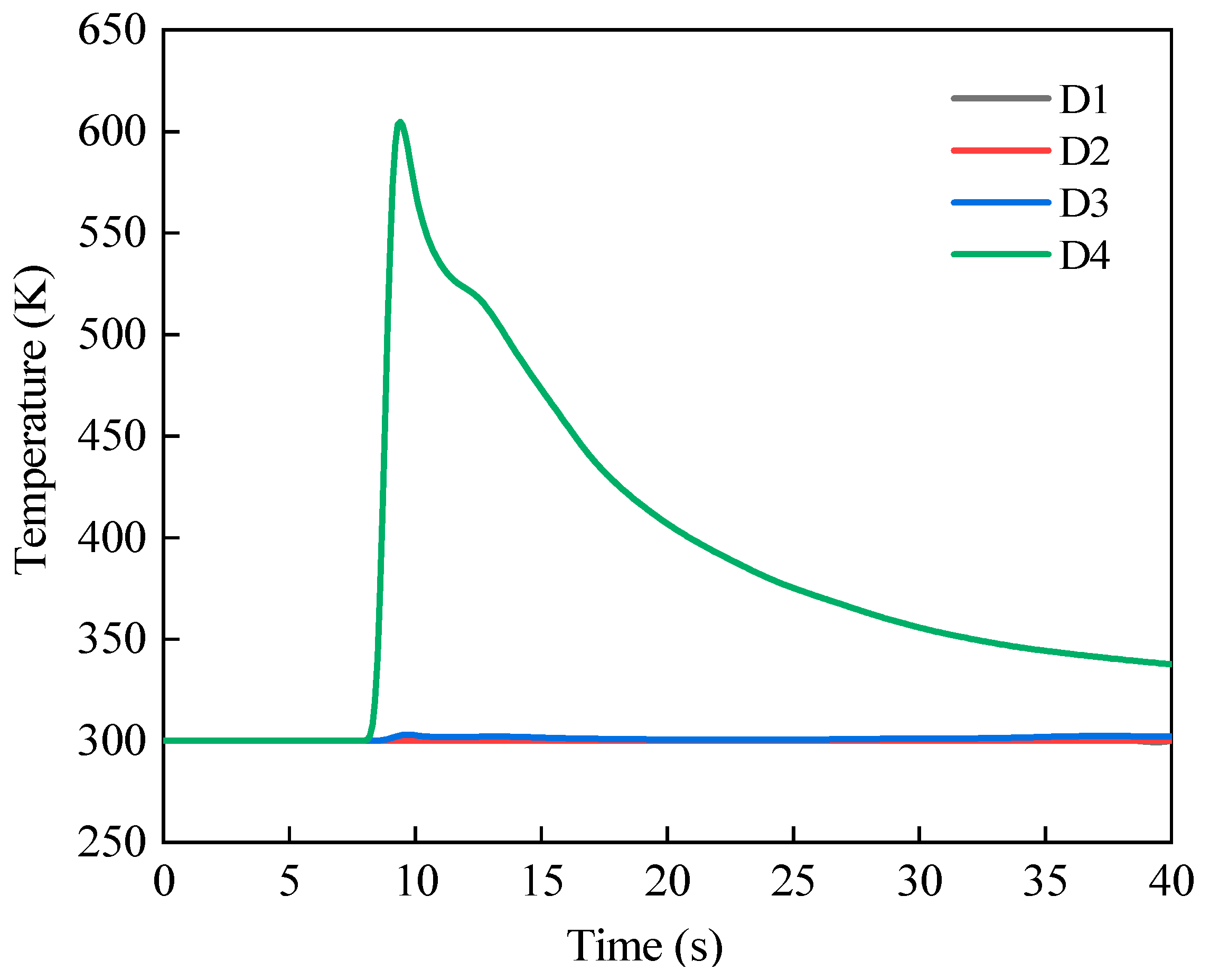
Figure 17: Monitoring-point data.
Based on an integral model and CFD numerical simulation, this study develops a full-process model of LH2 leakage, evaporation, dispersion, and combustion for station scenarios and systematically analyzes hydrogen dispersion and combustion behavior. The dispersion and combustion models are validated using experimental data. The results show that the developed model can reasonably reflect H2 cloud dispersion and flame-propagation characteristics. The main conclusions are as follows:
- (1)The source-term calculation shows a strongly transient LH2 evaporation process. The evaporation mass flow rate reaches a maximum of approximately 3.6 kg/s at 3.7–3.8 s, whereas the liquid-pool radius reaches its maximum value of approximately 1.2 m at 4.2 s. The evaporation mass flow rate decreases to a negligible level by approximately 7.5–7.6 s, while the residual liquid pool nearly disappears by approximately 8.5 s. Nevertheless, the previously formed H2 cloud continues to migrate and dilute for approximately 200 s, indicating that the dispersion hazard persists substantially longer than the active evaporation period.
- (2)Under the representative 6 kg LH2 release and 2 m/s wind condition, the flammable H2 cloud expands rapidly around the locomotive and toward the upper station region. In the non-ignited dispersion branch, at t = 9 s the 4 vol% H2 cloud front reaches 22.42 m and the cloud length reaches 28.92 m, with the flammable envelope extending around the locomotive. These results identify the source region, locomotive-adjacent region, and upper station space as important locations for hydrogen monitoring and emergency control.
- (3)The station geometry affects the migration and dilution of the H2 cloud. The maximum H2 volume fraction decreases from 0.056 at 40 s to 0.0184 at 80 s during the late dispersion stage. The roof promotes upper-level migration, while the locomotive and support columns modify the local flow and dilution patterns. Because these results are obtained for the present representative geometry and boundary conditions, the identified local retention characteristics should not be generalized to all station configurations.
- (4)Following ignition at t = 3.0 s in the ignition/combustion branch, the thermal hazard is concentrated mainly around the locomotive and upper station region during the early stage. The maximum flame temperature reaches 2193.5 K at t = 3.5 s and remains above 2000 K during t = 3–7 s. At about t = 40 s, the maximum temperature around the locomotive decreases to approximately 894 K, while the temperature in most regions approaches ambient conditions. These results indicate that early emergency response should prioritize locomotive-adjacent and upper station regions.
Acknowledgement:
Funding Statement: This work was financially supported by the Natural Science Foundation of Fujian Province (Grant No. 2025J0113).
Author Contributions: The authors confirm contribution to the paper as follows: Conceptualization, Dapeng Jin, Yuejiao Wang and Pengbo Yin; methodology, Dapeng Jin, Bin Liu and Pengbo Yin; software, Bin Liu and Pengbo Yin; validation, Dapeng Jin, Yichi Zhang, Sichao Zhang and Bin Liu; formal analysis, Yichi Zhang; investigation, Yichi Zhang and Sichao Zhang; resources, Yuejiao Wang and Pengbo Yin; data curation, Sichao Zhang; writing—original draft preparation, Dapeng Jin, Bin Liu and Pengbo Yin; writing—review and editing, Yuejiao Wang and Pengbo Yin; visualization, Yichi Zhang; supervision, Yuejiao Wang and Pengbo Yin; project administration, Yuejiao Wang; funding acquisition, Pengbo Yin. All authors reviewed and approved the final version of the manuscript.
Availability of Data and Materials: The authors confirm that the data supporting the findings of this study are available within the article.
Ethics Approval: Not applicable.
Conflicts of Interest: Given his role as [Editorial Board Members] of this journal, [Pengbo Yin] had no involvement in the peer review of this article and had no access to information regarding its peer review. Full responsibility for the editorial process for this article was delegated to another journal editor. The authors declare no other conflicts of interest.
Glossary
| Symbol | Description | Unit |
| Leakage mass flow rate | kg/s | |
| ρl | Density of liquid hydrogen | kg/m3 |
| Cd | Discharge coefficient | – |
| Ao | Leak-orifice area | m2 |
| Pt | Internal pressure of the storage tank | Pa |
| Pa | Ambient pressure | Pa |
| g | Gravitational acceleration | m/s2 |
| ht − ho | Height difference between the liquid level and the leak orifice | m |
| Mp | Mass of LH2 in the liquid pool | kg |
| Evaporation mass flow rate of the liquid pool | kg/s | |
| Ap | Liquid-pool area | m2 |
| R | Liquid-pool radius | m |
| δp | Equivalent thickness of the liquid pool | m |
| Lv | Latent heat of vaporization of LH2 | J/kg |
| Q′′g | Conductive heat flux transferred from the ground to the liquid pool | W/m2 |
| hc | Convective heat-transfer coefficient | W/(m2·K) |
| T∞ | Ambient air temperature | K |
| Tb | Boiling point of LH2 | K |
| εp | Surface emissivity of the liquid pool | – |
| σ | Stefan–Boltzmann constant | W/(m2·K4) |
| Ts | Surrounding-wall or environmental radiation temperature | K |
| kg | Thermal conductivity of the ground | W/(m·K) |
| Tg,0 | Initial ground temperature | K |
| αg | Thermal diffusivity of the ground | m2/s |
| t0 | Time when the liquid pool begins to form | s |
| Δt | Time correction used to avoid the initial heat-flux singularity | s |
| uin | Normal inlet velocity of hydrogen | m/s |
| ρH2(Tin) | Hydrogen density at the inlet temperature | kg/m3 |
| Tin | Hydrogen inlet temperature | K |
| ρ | Density of the gas mixture | kg/m3 |
| u | Velocity vector | m/s |
| Sm | Mass source term | kg/(m3·s) |
| p | Static pressure | Pa |
| τeff | Effective stress tensor | Pa |
| ueff | Effective dynamic viscosity | Pa·s |
| E | Total energy of the gas mixture | J/kg |
| keff | Effective thermal conductivity | W/(m·K) |
| T | Temperature | K |
| hi | Specific enthalpy of species (i) | J/kg |
| Ji | Diffusion flux of species (i) | kg/(m2·s) |
| Sh | Volumetric heat source | W/m3 |
| Srad | Radiation heat-transfer source term | W/m3 |
| Yi | Mass fraction of species (i) | – |
| Ri | Production rate of species (i) due to chemical reactions | kg/(m3·s) |
| Si | User-defined species source term | kg/(m3·s) |
| Deff,i | Effective diffusion coefficient of species (i) | m2/s |
| Di | Molecular diffusion coefficient of species (i) | m2/s |
| Sct | Turbulent Schmidt number | – |
| Ru | Universal gas constant | J/(mol·K) |
| Mi | Molar mass of species (i) | kg/mol |
| k | Turbulent kinetic energy | m2/s2 |
| ε | Turbulent dissipation rate | m2/s3 |
| Gk | Production of turbulent kinetic energy due to mean velocity gradients | – |
| YM | Contribution of fluctuating dilatation to turbulent dissipation | – |
| C1, C2, C3 | Constants of the turbulence model | – |
| μt | Turbulent viscosity | Pa·s |
| ST | Turbulent flame speed | m/s |
| SL | Laminar flame speed | m/s |
| u′ | Turbulent fluctuation velocity | m/s |
| Ct,n | Turbulent flame-speed model constants | – |
| Schem | Chemical-reaction heat source term | W/m3 |
| ωH2 | Hydrogen consumption rate due to reaction | kg/(m3·s) |
| ΔHc | Heat of combustion of hydrogen | J/kg |
| A(t) | Time-dependent gaseous-H2 inlet area | m2 |
| R(t) | Time-dependent liquid-pool radius | m |
References
1. Tackie-Otoo BN , Mahmoud M , Raza A . Renewable energy versus hydrogen energy: Assessing current needs for sustainable energy solutions. Energy Fuels. 2025; 39( 37): 17730– 62. doi:10.1021/acs.energyfuels.5c03207. [Google Scholar] [CrossRef]
2. Jasiński R , Michalak D , Ludwiczak A , Ziółkowski A , Wysibirski R . Hydrogen in transport: A comprehensive review of technologies, infrastructure, and future prospects. Energies. 2026; 19( 9): 2089. doi:10.3390/en19092089. [Google Scholar] [CrossRef]
3. Hassankhani Dolatabadi S , Vakili S , Ölcer AI . The role of green liquid hydrogen in sustainable transportation: Opportunities and barriers. In: Fuel cell and hydrogen technologies in maritime transportation. Berlin/Heidelberg, Germany: Springer; 2025. p. 57– 82. doi:10.1007/978-3-031-86110-9_3. [Google Scholar] [CrossRef]
4. Liu H , Wang W , Song H , Kuang T , Li Y , Guang Y . Consequence analysis of liquid hydrogen leakage from storage tanks at urban hydrogen refueling stations: A case study. Hydrogen. 2025; 6( 3): 58. doi:10.3390/hydrogen6030058. [Google Scholar] [CrossRef]
5. Trapani D , Marocco P , Gandiglio M , Santarelli M . Hydrogen leakages across the supply chain: Current estimates and future scenarios. Int J Hydrogen Energy. 2025; 145: 1084– 95. doi:10.1016/j.ijhydene.2025.06.103. [Google Scholar] [CrossRef]
6. Sun R , Pu L , Yu H , Dai M , Li Y . Modeling the diffusion of flammable hydrogen cloud under different liquid hydrogen leakage conditions in a hydrogen refueling station. Int J Hydrogen Energy. 2022; 47( 61): 25849– 63. doi:10.1016/j.ijhydene.2022.05.303. [Google Scholar] [CrossRef]
7. Liu X , Yuan B , Zeng S , Xu L , Song C , Xu N , et al. Study on liquid hydrogen leakage dispersion behavior and synergistic mitigation by barrier walls and air curtains in a hydrogen production and refueling station. Fire. 2026; 9( 6): 230. doi:10.3390/fire9060230. [Google Scholar] [CrossRef]
8. Menon SK , Kumar A , Mondal S . Advancements in hydrogen gas leakage detection sensor technologies and safety measures. Clean Energy. 2025; 9( 1): 263– 77. doi:10.1093/ce/zkae122. [Google Scholar] [CrossRef]
9. Wang Y , Zhao L , Lv X , He T . Numerical simulation and risk mitigation strategies for hydrogen leakage at vehicle hydrogenation stations. Int J Hydrogen Energy. 2025; 111: 735– 50. doi:10.1016/j.ijhydene.2025.02.230. [Google Scholar] [CrossRef]
10. Qu J , Zhou T , Zhao H , Deng J , Luo Z , Cheng F , et al. Risk analysis of hydrogen leakage at hydrogen producing and refuelling integrated station. Processes. 2025; 13( 2): 437. doi:10.3390/pr13020437. [Google Scholar] [CrossRef]
11. Han SH , Chang D , Kim JS . Experimental investigation of highly pressurized hydrogen release through a small hole. Int J Hydrogen Energy. 2014; 39( 17): 9552– 61. doi:10.1016/j.ijhydene.2014.03.044. [Google Scholar] [CrossRef]
12. Hao D , Wang X , Zhang Y , Wang R , Chen G , Li J . Experimental study on hydrogen leakage and emission of fuel cell vehicles in confined spaces. Automot Innov. 2020; 3( 2): 111– 22. doi:10.1007/s42154-020-00096-z. [Google Scholar] [CrossRef]
13. Kim J , Kim Y , Park B , Yoon U , Kang C . The effect of natural ventilation through roof vents following hydrogen leaks in confined spaces. Int J Hydrogen Energy. 2024; 50: 1395– 405. doi:10.1016/j.ijhydene.2023.11.048. [Google Scholar] [CrossRef]
14. Niu Y , Ma Z , Jiang B , Li P , Zuo J , Kou Y , et al. Experimental study on high-pressure hydrogen leakage and diffusion in full-scale hydrogen refueling stations. Int J Hydrogen Energy. 2025; 135: 351– 60. doi:10.1016/j.ijhydene.2025.05.026. [Google Scholar] [CrossRef]
15. Yao Y , Pan A , Hu M , Tan L , Wang Y , Zhan S . Experimental investigation on in-cabin hydrogen leakage and diffusion characteristics in hydrogen fuel cell vehicles. Fuel. 2026; 406: 136913. doi:10.1016/j.fuel.2025.136913. [Google Scholar] [CrossRef]
16. Gao X , Huang L , Ren J , Lan Y , Li M , Xiao H . Numerical study of the effect of barrier wall on liquid hydrogen leakage and dispersion. Int J Hydrogen Energy. 2025; 142: 460– 71. doi:10.1016/j.ijhydene.2025.01.031. [Google Scholar] [CrossRef]
17. Li J , Li D , Du X , Jin Z , Xin X . Study on the scope of impact of consequences of leakage of hydrogen blended with natural gas pipeline. J Loss Prev Process Ind. 2026; 99: 105810. doi:10.1016/j.jlp.2025.105810. [Google Scholar] [CrossRef]
18. Wu L , Qiao L , Fan J , Wen J , Zhang Y , Jar B . Investigation on leakage characteristics and consequences of hydrogen-blended gas pipelines based on CFD with the full multicomponent diffusion model. Renew Energy. 2025; 252: 123502. doi:10.1016/j.renene.2025.123502. [Google Scholar] [CrossRef]
19. Missey S . Simulation of flame propagation following liquid-hydrogen leak [ dissertation]. Toulouse, France: Université de Toulouse; 2026. doi:10.70675/DA007EE5ZFB52Z4B25ZB1E9Z89AC28B85C57. [Google Scholar] [CrossRef]
20. Zhang X , Xiao Y , Zhang J , Fang J , Xiong M , Zou J . Numerical simulation of hydrogen leakage, dispersion, and combustion in a hydrogen fuel cell bus maintenance workshop. Appl Therm Eng. 2026; 291: 130159. doi:10.1016/j.applthermaleng.2026.130159. [Google Scholar] [CrossRef]
21. Gong X , Li H , Li C , Kou M , Kong L , Liu H . Research on leakage and diffusion behavior of hydrogen doped natural gas in integrated pipeline corridors based on data drive. Sci Rep. 2025; 15( 1): 2860. doi:10.1038/s41598-025-86957-1. [Google Scholar] [CrossRef]
22. Yang Z , Chen Z , Han X , Chen G , Wang X . Numerical and experimental studies on the evolution characteristics of high-pressure hydrogen leakage and explosion accidents in hydrogen refueling stations. Int J Hydrogen Energy. 2025; 142: 580– 95. doi:10.1016/j.ijhydene.2025.04.420. [Google Scholar] [CrossRef]
23. Yang L , Shen J , Li J , Yin C , Lin Q , Shi L . Critical ventilation thresholds for hydrogen leakage of fuel cell vehicles in tunnels based on scaled experiment. Tunn Undergr Space Technol. 2026; 170: 107351. doi:10.1016/j.tust.2025.107351. [Google Scholar] [CrossRef]
24. Duan Q , Xin J , Zhang H , Hou Z , Duan P , Jin K , et al. Hydrogen leakage in underground garages: Impact of leakage locations on gas diffusion and safety considerations. J Energy Storage. 2025; 117: 116123. doi:10.1016/j.est.2025.116123. [Google Scholar] [CrossRef]
25. Yassin K , Kelm S , Reinecke EA . Numerical simulation of dispersion and ventilation of hydrogen clouds in case of leakage inside a large-scale industrial building. Hydrogen. 2025; 6( 2): 40. doi:10.3390/hydrogen6020040. [Google Scholar] [CrossRef]
26. Mo F , Liu B , Wang H , She X , Teng L , Kang X . Study on hydrogen dispersion in confined space with complex air supply and exhaust system. Int J Hydrogen Energy. 2022; 47( 67): 29131– 47. doi:10.1016/j.ijhydene.2022.06.238. [Google Scholar] [CrossRef]
27. Xu Q , Chen G , Xie M , Li X , Zhao Y , Su S , et al. Experimental and numerical studies on hydrogen leakage and dispersion evolution characteristics in space with large aspect ratios. J Clean Prod. 2024; 438: 140467. doi:10.1016/j.jclepro.2023.140467. [Google Scholar] [CrossRef]
28. Li J , Liu L , Bai W , Wu B , Dong J , Luo C , et al. Simulation and safety analysis of hydrogen leakage for hydrogen-powered vehicles in an enclosed parking garage. Int J Hydrogen Energy. 2025; 158: 150458. doi:10.1016/j.ijhydene.2025.150458. [Google Scholar] [CrossRef]
29. Chen G , Zhou S , Chen B , Xue R , Yang Y , Sun S . Numerical simulation of high-pressure hydrogen leakage and dispersion in tunnel environments for fuel cell locomotives. Int J Hydrogen Energy. 2025; 186: 152034. doi:10.1016/j.ijhydene.2025.152034. [Google Scholar] [CrossRef]
30. Magliano A , Perez Carrera C , Pappalardo CM , Guida D , Berardi VP . A comprehensive literature review on hydrogen tanks: Storage, safety, and structural integrity. Appl Sci. 2024; 14( 20): 9348. doi:10.3390/app14209348. [Google Scholar] [CrossRef]
31. Middha P , Ichard M , Arntzen BJ . Validation of CFD modelling of LH2 spread and evaporation against large-scale spill experiments. Int J Hydrogen Energy. 2011; 36( 3): 2620– 7. doi:10.1016/j.ijhydene.2010.03.122. [Google Scholar] [CrossRef]
32. Jin T , Wu M , Liu Y , Lei G , Chen H , Lan Y . CFD modeling and analysis of the influence factors of liquid hydrogen spills in open environment. Int J Hydrogen Energy. 2017; 42( 1): 732– 9. doi:10.1016/j.ijhydene.2016.10.162. [Google Scholar] [CrossRef]
33. Wang F , Meng Q , Zhao J , Wang X , Liu Y , Zhang Q . The turbulent Schmidt number for transient contaminant dispersion in a large ventilated room using a realizable k-ε model. Fluid Dyn Mater Process. 2024; 20( 4): 829– 46. doi:10.32604/fdmp.2023.026917. [Google Scholar] [CrossRef]
34. Launder BE , Spalding DB . The numerical computation of turbulent flows. In: Numerical prediction of flow, heat transfer, turbulence and combustion. Amsterdam, The Netherlands: Elsevier; 1983. p. 96– 116. doi:10.1016/b978-0-08-030937-8.50016-7. [Google Scholar] [CrossRef]
35. Patankar SV . Numerical heat transfer and fluid flow. Boca Raton, FL, USA: CRC Press; 1980. doi:10.1201/9781482234213. [Google Scholar] [CrossRef]
36. Chui EH , Raithby GD . Computation of radiant heat transfer on a nonorthogonal mesh using the finite-volume method. Numer Heat Transf Part B Fundam. 1993; 23( 3): 269– 88. doi:10.1080/10407799308914901. [Google Scholar] [CrossRef]
37. Witcofski R , Chirivella J . Experimental and analytical analyses of the mechanisms governing the dispersion of flammable clouds formed by liquid hydrogen spills. Int J Hydrogen Energy. 1984; 9( 5): 425– 35. doi:10.1016/0360-3199(84)90064-8. [Google Scholar] [CrossRef]
38. Middha P , Hansen OR . CFD simulation study to investigate the risk from hydrogen vehicles in tunnels. Int J Hydrogen Energy. 2009; 34( 14): 5875– 86. doi:10.1016/j.ijhydene.2009.02.004. [Google Scholar] [CrossRef]
39. ANSYS . ANSYS FLUENT UDF manual. Canonsburg, PA, USA: ANSYS Inc.; 2011. [Google Scholar]
40. Liu XX . Theoretical and experimental study on gas-pipeline leakage and dispersion in utility tunnels [ dissertation]. Beijing, China: Beijing University of Civil Engineering and Architecture; 2018. (In Chinese). [Google Scholar]
41. Liu Y , Zhang Y , Liu X , Liu Z , Che D . Experimental and numerical investigation on premixed H2/air combustion. Int J Hydrogen Energy. 2016; 41( 24): 10496– 506. doi:10.1016/j.ijhydene.2016.01.049. [Google Scholar] [CrossRef]
Cite This Article
 Copyright © 2026 The Author(s). Published by Tech Science Press.
This work is licensed under a Creative Commons Attribution 4.0 International License , which permits unrestricted use, distribution, and reproduction in any medium, provided the original work is properly cited.
 Downloads
 Citation Tools
