An Efficient Approach for Solving One-Dimensional Fractional Heat Conduction Equation

1  Introduction

The heat equation of one-dimension, initially investigated by Fourier in the 19th century, has remained a fundamental model for extensively studying linear and nonlinear parabolic partial differential equations (PDEs). There are various views of this exemplar, some of which have not yet been extended to space-variable case of multidimensions [1]. Notably, it covers discussions on free boundary value problems (BVPs) like the inverse problems, one-phase Stefan problem, and certain categories of ill-posed problems. The approach of implementing certain analytic tools to study this popular and widely applicable PDE makes it a worthwhile manual that aims to provide the basics of PDEs in simpler yet relevant situations, such as the one-dimensional heat equation [2].

In the last decades, there were several researchers who had studied the one-dimensional fractional heat conduction equation, but as far as we know, no one has investigated such a problem from the perspective of developing suitable fractional-order methods. This has actually motivated us to address this problem by the way of establishing a proper fractional approach that involves employing a combination of a novel fractional difference formula to approximate the Caputo differentiator of order α coupled with the modified three-point fractional formula to approximate the Caputo differentiator of order 2α, where 0<α≤1. As we have mentioned a little while ago, the fractional heat conduction equation has attracted the interest of scholars in composite medium. For instance, the fractional diffusion equation of one dimension was solved analytically and numerically in a composite medium consisting of two layers in contact by Ilic et al. [3]. The fractional heat conduction problem was also studied by Povstenko in a composite medium with a spherical inclusion and in a composite medium consisting of two semi-infinite regions being in perfect thermal contact [4,5]. The one-dimensional fractional thermal diffusion equation was set up and consequently solve by Jiang et al. in a composite medium [6]. With the use of the Levenberg-Marquardt iterative method, the inverse problem of parameter estimation for time-fractional heat conduction equation was studied by means of using carbon-carbon experimental data in a composite medium by Zhuang et al. [7]. The time-fractional inverse heat conduction problem in the sense of Caputo operator was further investigated on a finite slab in the presence of measured data by Murio [8]. The inverse heat conduction problem was additionally explored in processed meat by Ghazizadeh et al. [9]. More recently, Yu et al. proposed a novel time-fractional heat conduction model in the hyperthermia experiment for the bi-layered spherical tissue, and then they estimated some unknown fractional parameters using a proper numerical method [10].

Fractional calculus and fractional partial differential equations (FPDEs) have garnered growing consideration across multiple scientific fields for the past decades [11–13]. Replacing the derivative of integer-order in energy conservation models, momentum or standard mass with a fractional-order derivative enables up-scaling of local variations that are often challenging to exclusively measure [14,15]. This leads to non-local FPDEs with temporally or spatially averaged parameters, offering an efficient means to capture more rich dynamics of the considered problem [16–18]. Fractional differential equations (FDEs) commonly describe the relationship between an unknown function and its derivatives, typically involving fractional derivatives of a single independent variable. This type of equations can be further categorized into fractional initial value problems (FIVPs) and fractional boundary value problems (FBVPs) [19]. Analytical solutions for practical problems stemming from limited FIVPEs and FBVPs are proposed in conjunction with specific analytical methods. Homotopy perturbation technique, Adomian decomposition method and variational iteration method are, for instance, some of these methods [20]. In the same regards, various numerical approaches are regarded immensely helpful tools for promptly finding solutions for numerous linear and nonlinear FIVPEs and FBVPs problems, especially when combined them with code producing. Many investigators have advanced numerous numerical methods for solving such problems. Galerkin finite element approach, finite difference method, collocation method, spectral method, Gegenbauer-based Nyström method, fractional Euler’s method, modified fractional Euler method, improved modified fractional Euler method and wavelet method are, for instance, some of these numerical methods, see [20–26]. The problem here is to find a numerical solution of the one-dimensional fractional heat conduction equation. From a mathematical point of view, this is a moving boundary problem and it is difficult to obtain its exact solutions. For fractional moving boundary problems, some researchers attempted to present proper analytical solutions for different types of those problems, see [27] and the references therein.

The rest of this article is arranged as follows: In the next section, we recall the most important preliminaries connected with the fractional calculus. In Section 3, we first establish a novel fractional difference formula to approximate the Caputo differentiator of order α, and then combine it with the so-called modified three-point fractional formula to approximate the Caputo differentiator of order 2α, where 0<α≤1. This would help us in solving the one-dimensional fractional heat conduction equation numerically. In Section 4, we validate our proposed numerical approach by providing several illustrative examples, and finally we provide the conclusion of this work.

2  Basic Definitions and Facts

In this section, we review a few primary definitions and important preliminary concepts related to fractional calculus. These key concepts serve as a foundation for our principal results that will be presented later.

Definition 2.1. [12,28] The Riemann–Liouville integrator in its fractional case of a function h(t) might be outlined as

Jμh(t)=1Γ(μ)∫0th(s)(t−s)μ−1ds,(1)

where μ>0 and t>0.

In the subsequent lines, we review specific features of Riemann–Liouville integrator for fulfillment:

1)J0h(t)=h(t).(2)

2)Jμ(t−a)γ=Γ(γ+1)Γ(μ+γ+1)(t−a)μ+γ,a∈R, γ≥−1.(3)

3)JμJβh(t)=Jμ+βh(t),μ,β≥0.(4)

4)JμJβh(t)=JβJμh(t),μ,β≥0.(5)

Definition 2.2. [12,28] The Caputo differentiator of a function h(t) might be outlined as

D∗μh(t)=1Γ(m−μ)∫0t(t−s)m−μ−1h(m)(s)ds(6)

where m−1<μ≤m, t>0 and m∈N.

Some of Caputo differentiator properties are outlined in the following content [12,28]:

1)D∗μc=0,where c is constant.(7)

2)D∗μ(t−a)ρ=Γ(ρ+1)Γ(ρ−μ+1)(t−a)ρ−μ, a∈R,ρ>μ−1.(8)

3)D∗μ(ω1ψ1(t)+ω2ψ2(t))=ω1D∗μ(ψ1(t))+ω2D∗μ(ψ2(t)), where μ and ω are constant.(9)

Along the same lines, we remember in what follows some further characteristics associated with the composition Riemann–Liouville integrator with Caputo differentiator [12,28]:

D∗αJαh(t)=h(t),(10)

and

JαD∗αh(t)=h(t)−∑i=1nhi(0+)tii!,(11)

where n−1<α≤n, n∈N, and t>0.

Definition 2.3. [12,28] The Caputo differentiator could be described in terms of the Riemann–Liouville integrator of a function h(t) as

D∗μh(t)=Dm[Jρh(t)],(12)

where ρ=m−μ, 0<ρ<1 and m is the smallest integral greater than μ>0.

In the following lines, we remind one significant result that plays a crucial role in deriving the principal findings of this work, the generalized Taylor’s theorem [12].

Theorem 2.1. [12] (Generalized Taylor’s Theorem) Assume that D∗kαf(x)∈Cn+1(a,b], where 0<α≤1 and k=0,1,⋯,n+1. Then the function f can be expanded about x=x0 as follows:

f(x)=∑i=0n(x−x0)iαΓ(iα+1)D∗iαf(x0)+(x−x0)(n+1)αΓ((n+1)α+1)D∗(n+1)αf(ξ),(13)

where x∈(a,b) and a<ξ<x.

3  Numerical Approach

In this part, we intend to introduce the major findings of this work. To do so, we first establish a highly significant result concerning the Caputo fractional differentiator.

Lemma 3.1. Let f∈C2[a,b] and x0,x1 be two distinct points in the interval [a,b] such that a=x0<x1=x0+h=b with h>0. Then the fractional version of the difference method for approximating Caputo differentiator might be outlined by

D∗αf(x0)=Γ(α+1)h(f(x1)−f(x0))−hΓ(α+1)Γ(2α+1)D∗2αf(ξ),(14)

where α∈(0,1], for some ξ∈(a,b).

Proof. Based on Theorem 2.1, one might expand f about x0 as follows:

f(x)=f(x0)+D∗αf(x0)(x−x0)Γ(α+1)+D∗2αf(ξ)(x−x0)2Γ(2α+1),(15)

for some unknown value of ξ∈(a,b). Now, by substituting x1 instead of x, we get

f(x1)=f(x0)+D∗αf(x0)(x1−x0)Γ(α+1)+D∗2αf(ξ)(x1−x0)2Γ(2α+1),(16)

or

f(x1)=f(x0)+D∗αf(x0)hΓ(α+1)+D∗2αf(ξ)h2Γ(2α+1),(17)

This implies

hΓ(α+1)D∗αf(x0)=f(x1)−f(x0)−h2Γ(2α+1)D∗2αf(ξ),(18)

which immediately yields

D∗αf(x0)=Γ(α+1)h(f(x1)−f(x0))−hΓ(α+1)Γ(2α+1)D∗2αf(ξ),(19)

or approximately as

D∗αf(x0)≈Γ(α+1)h(f(x1)−f(x0)),(20)

with truncation error

e=−hΓ(α+1)Γ(2α+1)D*2αf(ξ).

Recently, an important result was obtained in [29] in order to approximate the Caputo differentiator. The derivation of this result was inspired by a similar approach used in [30], and it was termed the modified three-point fractional formula. However, we recall this result below for completeness.

Theorem 3.1. [29] Let f∈C3[a,b] and x0,x1,x2 be three distinct nodes in the interval [a,b] in which a=x0<x1=x0+h<x2=x0+2h=b with h>0. Then to approximate the Caputo differentiator, we have the modified three-point fractional formula, which has the form

D∗αf(x)=x2−αh2Γ(3−α)(f(x0)−2f(x1)+f(x2))−x1−α2h2Γ(2−α)(f(x0)(x1+x2)−2f(x1)(x0+x2)+f(x2)(x0+x1))+f(3)(ξ)6(6Γ(4−α)x3−α−2(x0+x1+x2)Γ(3−α)x2−α+(x0x1+x0x2+x1x2)Γ(2−α)x1−α),(21)

where a<ξ<x and x∈(a,b).

As a result of Theorem 3.1 that concerns with the modified three-point fractional formula for approximating Caputo differentiator D∗α, where 0<α≤1, we can now outline the next result that can aid in approximating the Caputo differentiator D∗2α, where 0<α≤1.

Corollary 3.1. Let f∈C3[a,b] and x0,x1,x2 be three distinct nodes in [a,b] in which a=x0<x1=x0+h<x2=x0+2h=b with h>0. Then to approximate Caputo differentiator D∗2α, we have the modified three-point fractional formula, which has the form

D∗2αf(x1)=x12−2αh2Γ(3−2α)(f(x0)−2f(x1)+f(x2))+f(3)(ξ)6(6x13−2αΓ(4−2α)−2(x0+x1+x2)Γ(3−2α)x12−2α),(22)

where 0<α≤1, a<ξ<x, and x∈(a,b).

Proof. This result is immediately yielded by just operating the Caputo differentiator (2.2) to the fractional formula (21) once again, and by substituting x1 instead of x into the result. ■

From now on, we aim to investigate the so-called one-dimensional heat conduction equation. The classical form of this kind of equations can be given by

∂u∂t=β∂2u∂x2, β>0,

with boundary conditions

u(0,t)=0, u(L,t)=0, t>0, L>0,

and with initial condition

u(x,0)=g(x), 0≤x≤L.

In fact, the above problem can be expressed in its corresponding fractional-order case as follows:

∂αu∂tα=β∂2αu∂x2α, β>0,(23)

with boundary conditions

u(0,t)=0, u(L,t)=0, t>0, L>0,

and with initial condition

u(x,0)=g(x), 0≤x≤L.

To solve problem (23), we will utilize the fractional difference formula for approximating the Caputo differentiator, as presented in Theorem 3.1, in conjunction with the modified three-points fractional formula for approximating Caputo differentiator of order 2α, as given in Corollary 3.1. To do so, we let nt=b1−a1ht and nx=b2−a2hx in which the intervals [a1,b1] and [a2,b2] are divided respectively as a1=t0<t1=t0+ht<t2=t0+2ht<⋯<tnt=t0+ntht=b1 with ht>0 and a2=x0<x1=x0+hx<x2=x0+2hx<⋯<xnx=x0+nxhx=b2 with hx>0. In the specific context of t lying in the interval [a1,b1] and x lying in the interval [a2,b2], the points of intersection are referred to as mesh points, nodal points, or grid points. These points can be represented respectively as tk=kht and xj=jhx, for k=0,1,…,nt and j=0,1,…,nx. Now, by employing the two formulas in (14) and (22), we can numerically rewrite problem (23) as follows:

Γ(α+1)ht(ujk+1−ujk)=β(xj2−2αhx2Γ(3−2α))(uj+1k+1−2ujk+1+uj−1k+1),(24)

for j=1,2,⋯,nx and k=0,1,2,⋯,nt. This consequently implies

ujk=ujk+1−htβxj2−2αhx2Γ(α+1)Γ(3−2α)(uj+1k+1−2ujk+1+uj−1k+1).(25)

This equality can be written in the form

ujk=(1+2s)ujk+1−s(uj+1k+1+uj−1k+1),(26)

where

s=htβxj2−2αhx2Γ(α+1)Γ(3−2α).

Now, with the use of (26), we can infer the following states

j=1,       (1+2s)u1k+1−s(u2k+1+u0k+1)=u1kj=2,       (1+2s)u2k+1−s(u3k+1+u1k+1)=u2kj=3,       (1+2s)u3k+1−s(u4k+1+u2k+1)=u3k⋮j=l,       (1+2s)ulk+1−s(ul+1k+1+ul−1k+1)=ulk,

where l=nx−1. In fact, the above equations can be rewritten in a matrix form as follows:

[1+2s−s0…00−s1+2s−s…000−s1+2s…00⋮⋮⋮⋱⋮⋮000…1+2s−s000…−s1+2s][u1k+1u2k+1u3k+1⋮ul−1k+1ulk+1]=[u1ku2ku3k⋮ul−1kulk]+[u0k+100⋮0ul+1k+1],

for k=0,1,2,…,nt. In other words, the above system can be written in the form

Al×lU→l×1k+1=U→l×1k+Bl×1,

where

A=[1+2s−s0…00−s1+2s−s…000−s1+2s…00⋮⋮⋮⋱⋮⋮000…1+2s−s000…−s1+2s],U→k+1=[u1k+1u2k+1u3k+1⋮ul−1k+1ulk+1],

and

U→k=[u1k+100⋮0ulk+1], B=[u0k+100⋮0ul+1k+1].

The system described above can be solved algebraically using MATLAB to obtain the desired approximate solution for the intended problem as MATLAB provides powerful numerical and computational tools that are well-suited for solving systems of equations and obtaining approximate solutions efficiently and accurately.

4  Illustrative Examples

In this part, we intend to verify the effectiveness of our proposed approach. Figures and tables are utilized to display and compare the gained findings.

Example 4.1. Consider the following fractional heat conduction equation:

∂αu∂tα=β∂2αu∂x2α,(27)

with boundary conditions

u(0,t)=0, u(1,t)=0, t>0,

and with initial condition

u(x,0)=sin(π4x)(1+2cos(π4x)).

It should be noted that the analytical solution of problem (27) when β=4π2 and α=1 is given by

u(x,t)=e−tsin(π2x)+e(−t4)sin(π4x).(28)

In particular, the above analytical solution (28) can be plot as shown in Fig. 1. In this connection, when we apply on the proposed numerical approach discussed in Section 3 with letting α=1, we can generate an approximate numerical solution of problem (27) as it can be seen in Fig. 2. With the aim of validating our proposed approach, we perform a graphical comparison between the analytical and numerical solutions when α=1 as it can be seen in Fig. 3. In addition, we also depict the absolute values of the errors gained from making such comparison, which can be respectively shown in Fig. 4 and Table 1 for x∈[0,2] and t∈[0,0.12] with step sizes hx=0.04 and ht=0.04.

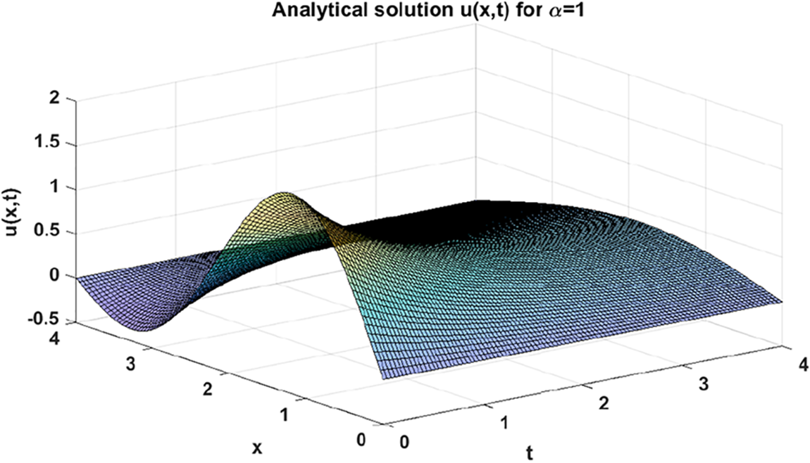
Figure 1: Analytical solution u(x,t) of problem (27) when β=4π2 and α=1

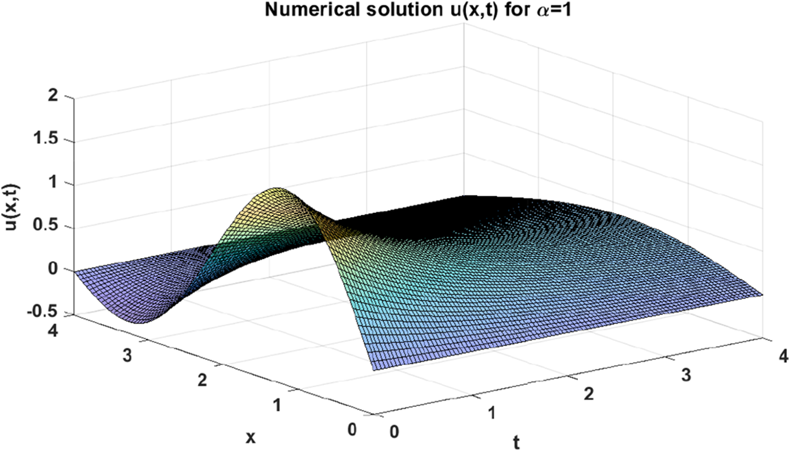
Figure 2: Numerical solution u(x,t) of problem (27) when β=4π2 and α=1

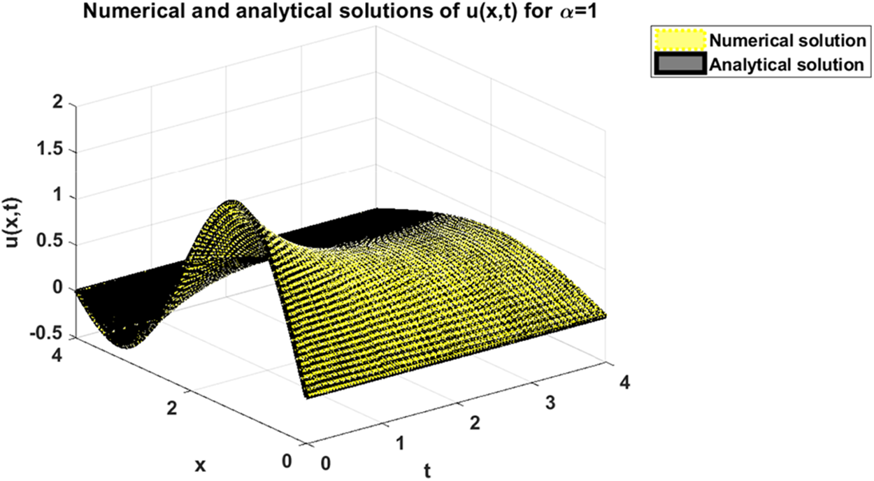
Figure 3: Comparison between numerical and analytical solutions of problem (27) when α=1

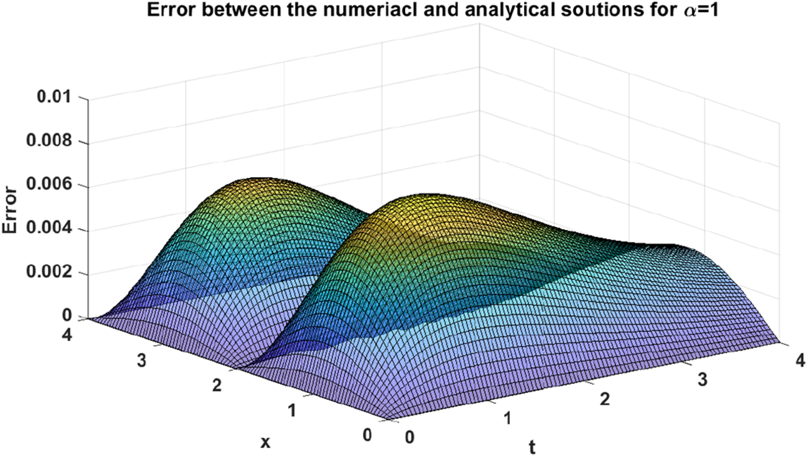
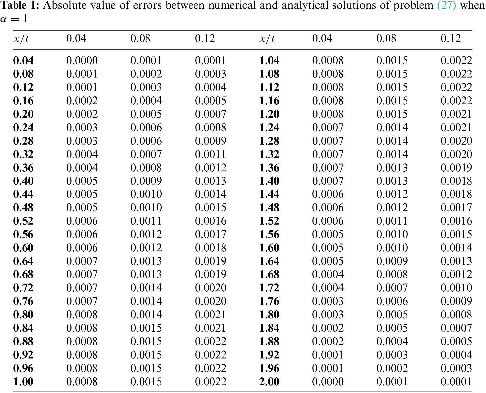
Figure 4: Absolute value of errors between numerical and analytical solutions of problem (27) when α=1

At this point, for the purpose of illustrating the dynamics of the numerical solution of problem (27) when, e.g., α=0.75, we plot a set of figures shown below. In particular, Fig. 5 depicts the numerical solution of problem (27) when α=0.75. Fig. 6 shows the dynamics of the solution u(x,t) with respect to the variable x, while Fig. 7 shows the dynamics of the same solution with respect to the variable t. Finally, a variation in the dynamics of the numerical solution when α=0.75 and the analytical solution when α=1 is shown in Fig. 8.

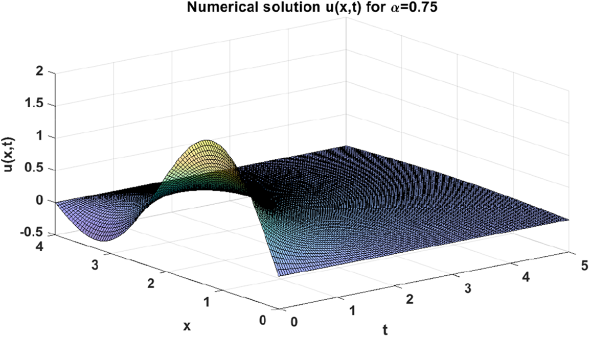
Figure 5: Numerical solution of problem (27) when α=0.75

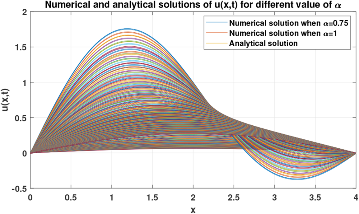
Figure 6: Dynamics of the numerical solution of problem (27) w.r.t x when α=0.75,1

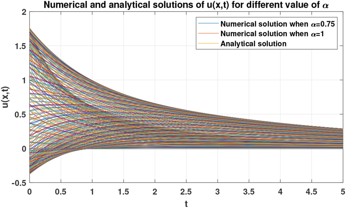
Figure 7: Dynamics of the numerical solution of problem (27) w.r.t t when α=0.75,1

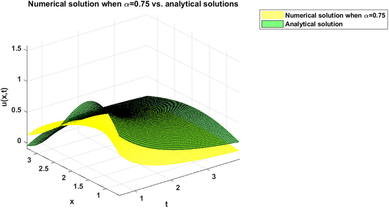
Figure 8: Comparison between numerical solution when α=0.75 and analytical solution (28) of problem (27)

Example 4.2. Consider the following fractional heat conduction equation:

∂αu∂tα=β∂2αu∂x2α,(29)

with boundary conditions

u(0,t)=0, u(1,t)=0, t>0,

and with initial condition

u(x,0)=u(x,0)=sin(πx).

The analytical solution of problem (29) when β=0.05 and α=1 is given by

u(x,t)=sin(πx)e−0.05π2t.(30)

The above analytical solution (28) can be plot as shown in Fig. 9. Now, when we apply on the proposed numerical approach discussed in Section 3 with letting α=1, we can generate an approximate numerical solution of problem (29) as it can be seen in Fig. 10. For the purpose of validating our proposed approach, we perform a graphical comparison between the analytical and numerical solutions when α=1 as it can be seen in Fig. 11. In addition, we also depict the absolute values of the errors gained from making such comparison, which can be respectively shown in Fig. 12 and Table 2 for x∈[0,2] and t∈[0,0.12] with step sizes hx=0.04 and ht=0.04.

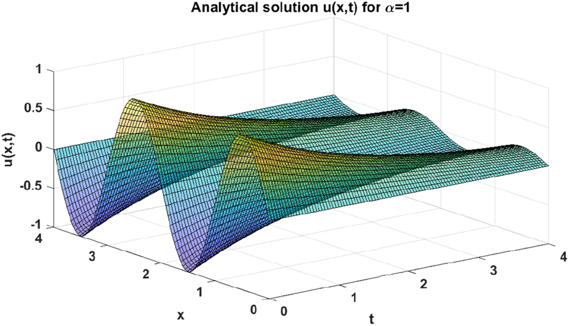
Figure 9: Analytical solution u(x,t) of problem (29) when β=0.05 and α=1

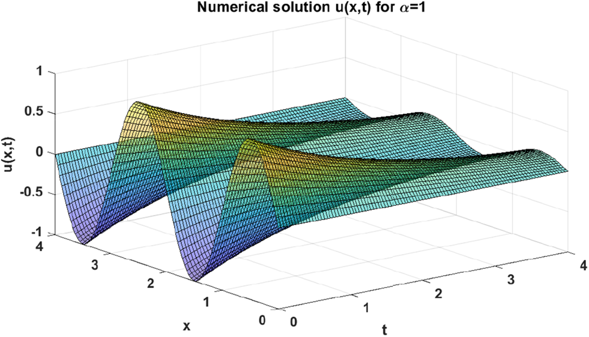
Figure 10: Numerical solution u(x,t) of problem (29) when β=0.05 and α=1

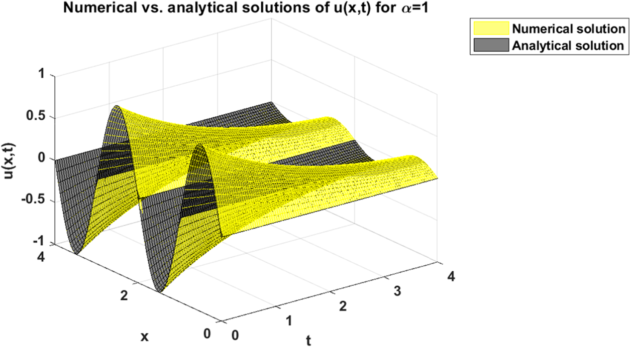
Figure 11: Comparison between numerical and analytical solutions of problem (29) when α=1

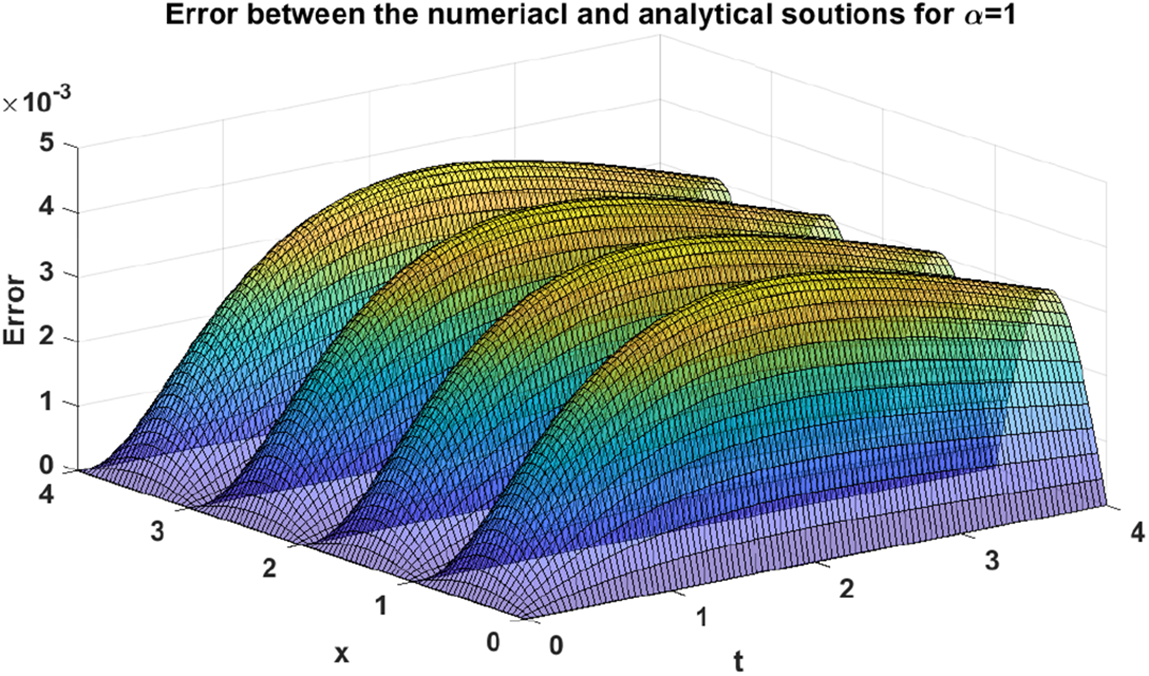
Figure 12: Absolute value of errors between numerical and analytical solutions of problem (29) when α=1

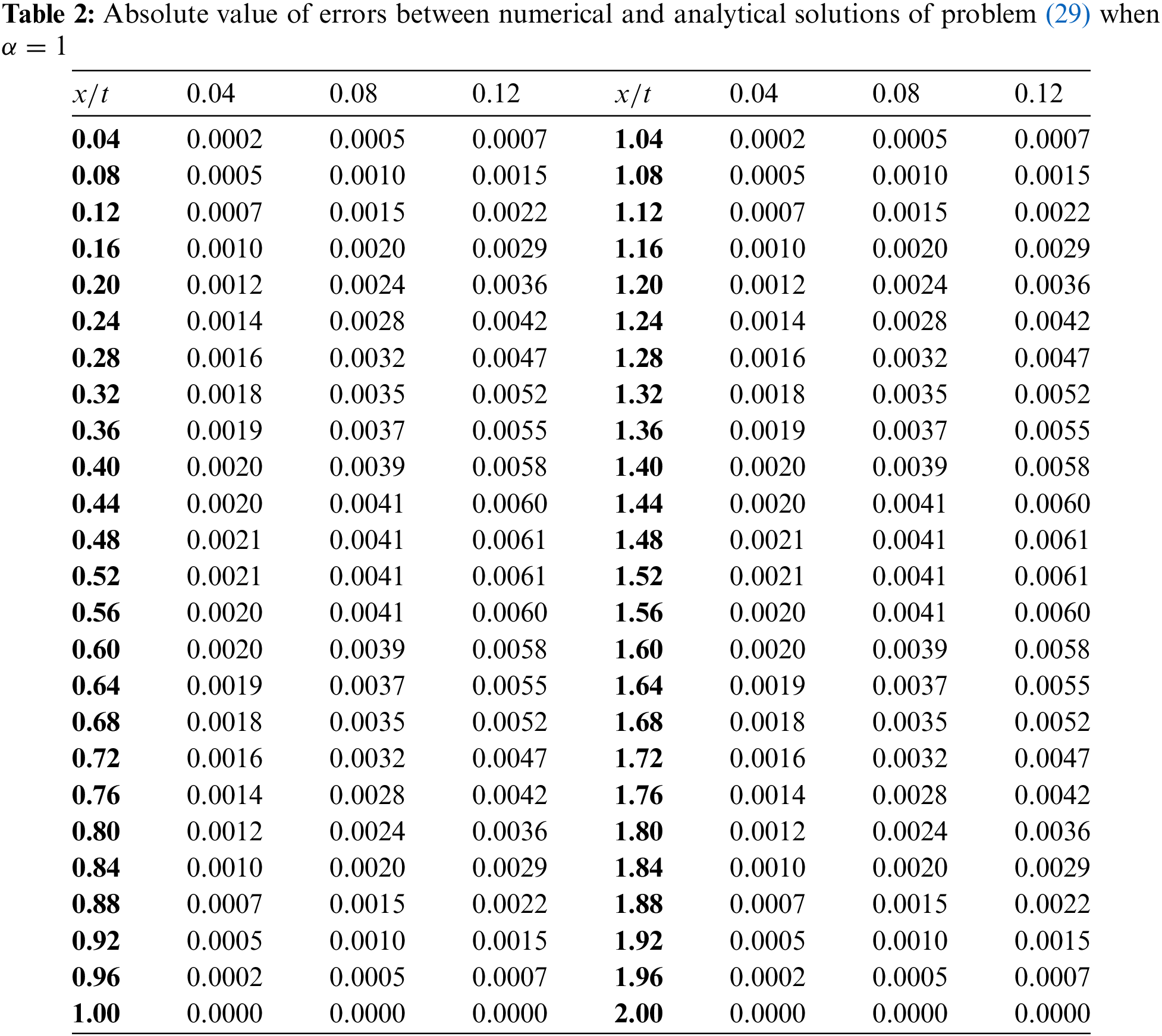
With the aim of illustrating the dynamics of the numerical solution of problem (29) when, e.g., α=0.75, we plot a set of figures shown below. In particular, Fig. 13 depicts the numerical solution of problem (29) when α=0.75. Fig. 14 shows the dynamics of the solution u(x,t) with respect to the variable x, while Fig. 15 shows the dynamics of the same solution with respect to the variable t. Finally, a variation in the dynamics of the numerical solution when α=0.75 and the analytical solution when α=1 is shown in Fig. 16.

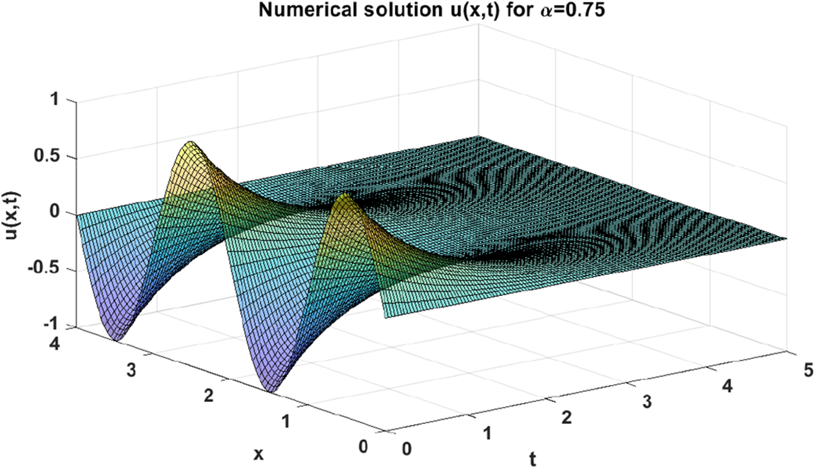
Figure 13: Numerical solution of problem (29) when α=0.75

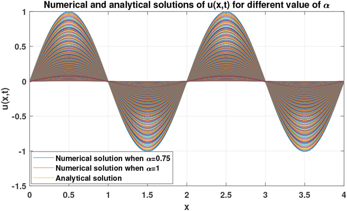
Figure 14: Dynamics of the numerical solution of problem (29) w.r.t x when α=0.75,1

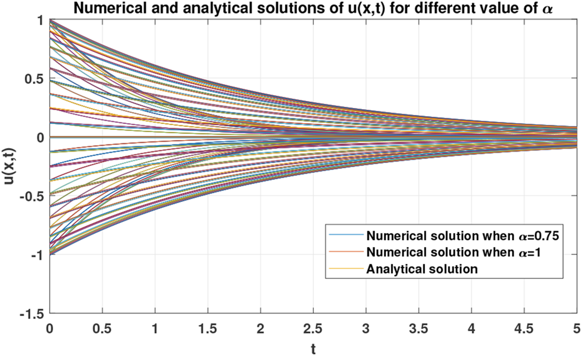
Figure 15: Dynamics of the numerical solution of problem (29) w.r.t t when α=0.75,1

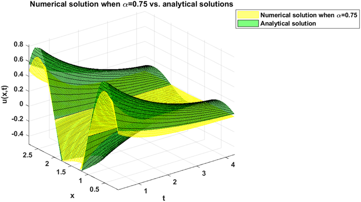
Figure 16: Comparison between numerical solution when α=0.75 and analytical solution (30) of problem (29)

5  Conclusion

Based on the examples and figures presented earlier, it is evident that the proposed formula offers a reliable approximation for the heat conduction equation in the fractional-order when compared with the provided analytical values. This observation suggests that the formula holds promise for various applications, particularly those involving ordinary and partial differential equations. With this encouraging outcome, there is potential for applying the formula in numerous real-world scenarios, enabling more efficient and accurate solutions to similar problems. In particular, our future direction will be focused on addressing similar problems to ours including solving two-dimensional fractional heat conduction equation, one-dimensional fractional wave equation, two-dimensional fractional wave equation, etc.

Acknowledgement: The authors wish to express their appreciation to the reviewers for their helpful suggestions which greatly improved the presentation of this paper.

Funding Statement: The authors received no specific funding for this study.

Author Contributions: The authors confirm contribution to the paper as follows: study conception and design: Iqbal M. Batiha, Shaher Momani; data collection: Hamza S. Kanaan; analysis and interpretation of results: Iqbal M. Batiha, Iqbal H. Jebril, Mohammad Zuriqat; draft manuscript preparation: Hamza S. Kanaan, Shaher Momani. All authors reviewed the results and approved the final version of the manuscript.

Availability of Data and Materials: Data sharing is not applicable to this article as no new data were created or analyzed in this study.

Conflicts of Interest: The authors declare that they have no conflicts of interest to report regarding the present study.

References

1. He, J. (2019). A simple approach to one-dimensional convection-diffusion equation and its fractional modification for E reaction arising in rotating disk electrodes. Journal of Electroanalytical Chemistry, 854(1), 1–2. [Google Scholar]

2. Cannon, J. (1984). The one dimensional heat equation. UK: Cambridge University Press. [Google Scholar]

3. Ilic, M., Turner, I., Liu, F., Anh, V. (2010). Analytical and numerical solutions of a one dimensional fractional in space diffusion equation in a composite medium. Applied Mathematics and Computation, 216(8), 2248–2262. [Google Scholar]

4. Povstenko, Y. (2013). Fractional heat conduction in infinite one dimensional composite medium. Journal of Thermal Stresses, 36(4), 351–363. [Google Scholar]

5. Povstenko, Y. (2013). Fractional heat conduction in an infinite medium with a spherical inclusion. Entropy, 15(10), 4122–4133. [Google Scholar]

6. Jiang, X., Chen, S. (2015). Analytical and numerical solutions of time fractional anomalous thermal diffusion equation in composite medium. ZAMM Zeitschrift fur Angewandte Mathematik und Mechanik, 95(2), 156–164. [Google Scholar]

7. Zhuang, Q., Yu, B., Jiang, X. (2015). An inverse problem of parameter estimation for timefractional heat conduction in a composite medium using carbon carbon experimental data. Physica B: Condensed Matter, 456(1), 9–15. [Google Scholar]

8. Murio, D. (2008). Time fractional IHCP with Caputo fractional derivatives. Computers and Mathematics with Applications, 56(9), 2371–2381. [Google Scholar]

9. Ghazizadeh, H., Azimi, A., Maerefat, M. (2012). An inverse problem to estimate relaxation parameter and order of fractionality in fractional single phase lag heat equation. International Journal of Heat and Mass Transfer, 55(7–8), 2095–2101. [Google Scholar]

10. Yu, B., Jiang, X. (2019). Temperature prediction by a fractional heat conduction model for the bilayered spherical tissue in the hyperthermia experiment. International Journal of Heat and Mass Transfer, 145(1), 105990. [Google Scholar]

11. Dababneh, A., Sami, B., Abu Hammad, M., Zraiqat, A. (2020). A new impulsive sequential multiorders fractional differential equation with boundary conditions. Journal of Mathematical and Computational Science, 10(6), 2871–2890. [Google Scholar]

12. Bahia, G., Ouannas, A., Batiha, I., Odibat, Z. (2021). The optimal homotopy analysis method applied on nonlinear time fractional hyperbolic partial differential equations. Journal of Mathematical and Computational Science, 37(3), 2008–2022. [Google Scholar]

13. Chebana, Z., Oussaeif, T., Ouannas, A., Batiha, I. (2022). Solvability of Dirichlet problem for a fractional partial differential equation by using energy inequality and Faedo Galerkin method. Innovative Journal of Mathematics, 1(1), 34–44. [Google Scholar]

14. He, J., Ji, F. (2019). Two scale mathematics and fractional calculus for thermodynamics. Thermal Science, 23(4), 2131–2133. [Google Scholar]

15. Ahmad, H., Khan, T., Stanimirovic, P., Ahmad, I. (2020). Modified variational iteration technique for the numerical solution of fifth order KdV-type equations. Journal of Applied and Computational Mechanics, 6(1), 1220–1227. [Google Scholar]

16. Hammachukiattikul, P., Mohanapriya, A., Ganesh, A., Rajchakit, G., Govindan, V. et al. (2020). A study on fractional differential equations using the fractional Fourier transform. Advances in Difference Equations, 2020(1), 691. [Google Scholar]

17. Maitama, S. (2018). Local fractional natural Homotopy perturbation method for solving partial differential equations with local fractional derivative. Progress in Fractional Differentiation and Applications, 4(3), 219–228. [Google Scholar]

18. Zhang, J., Zhang, X., Yang, B. (2018). An approximation scheme for the time fractional convection diffusion equation. Applied Mathematics and Computation, 335(1), 305–312. [Google Scholar]

19. Agarwal, R., Sonal, J. (2018). Mathematical modeling and analysis of dynamics of cytosolic calcium ion in astrocytes using fractional calculus. Journal of Fractional Calculus and Applications, 9(2), 1–12. [Google Scholar]

20. Pitolli, F. (2020). On the numerical solution of fractional boundary value problems by a spline quasi interpolant operator. Axioms, 9(2), 61. [Google Scholar]

21. Odibat, Z., Momani, S. (2008). An algorithm for the numerical solution of differential equations of fractional order. Journal of Applied Mathematics and Informatics, 26(1), 15–27. [Google Scholar]

22. Batiha, I., Bataihah, A., Al Nana, A., Shameseddin, A., Jebril, I. et al. (2023). A numerical scheme for dealing with fractional initial value problem. ICIC Express Letters, 19(3), 763–774. [Google Scholar]

23. Batiha, I., Abubaker, A., Jebril, I., Al Shaikh, S., Matarneh, K. (2023). New algorithms for dealing with fractional initial value problems. Axioms, 12(5), 488. [Google Scholar]

24. Memon, Z., Chandio, M., Qureshi, S. (2015). On consistency, stability and convergence of a modified ordinary differential equation solver. Sindh University Research Journal, 47(4), 631–636. [Google Scholar]

25. Islam, M. (2015). Accuracy analysis of numerical solutions of initial value problems (IVP) for ordinary differential equations (ODE). IOSR Journal of Mathematics, 11(3), 18–23. [Google Scholar]

26. Pandey, P. (2018). A new computational algorithm for the solution of second order initial value problems in ordinary differential equations. Applied Mathematics and Nonlinear Sciences, 3(1), 167–174. [Google Scholar]

27. Li, X., Wang, S., Zhao, M. (2013). Two methods to solve a fractional single phase moving boundary problem. Central European Journal of Physics, 11(10), 1387–1391. [Google Scholar]

28. Batiha, I., El Khazali, R., AlSaedi, A., Momani, S. (2018). The general solution of singular fractional order linear time invariant continuous systems with regular pencils. Entropy, 20(6), 400. [Google Scholar] [PubMed]

29. Batiha, I., Alshorm, S., Ouannas, A., Momani, S., Ababneh, O. et al. (2022). Modified three point fractional formulas with Richardson extrapolation. Mathematics, 10(19), 3489. [Google Scholar]

30. Burden, R. L., Faires, J. D. (2010). Numerical analysis, 9th edition. Bosto, USA: Cengage Learning. [Google Scholar]