
 Submit a Paper
 Propose a Special lssue
 Open Access
ARTICLE
Experimental Evaluation of Individual Hotspots of a Multicore Microprocessor Using Pulsating Heat Sources
1 Department of Mechanical Engineering, University Centre of United Metropolitan Faculties, São Paulo, Brazil
2 Department of Mechanical Engineering, University of São Paulo, São Paulo, Brazil
* Corresponding Author: Flávio Augusto Sanzovo Fiorelli. Email:
Frontiers in Heat and Mass Transfer 2023, 21, 427-443. https://doi.org/10.32604/fhmt.2023.041917
Received 11 May 2023; Accepted 14 July 2023; Issue published 30 November 2023
 View Full Text
 Download PDF
Abstract
The present work provides an experimental and numerical procedure to obtain the geometrical position of the hotspots of a microprocessor using the thermal images obtained from the transient thermal response of this processor subject to pulsating stress tests. This is performed by the solution of the steady inverse heat transfer problem using these thermal images, resulting in qualitative heat source distributions; these are analyzed using the mean heat source gradients to identify the elements that can be considered hotspots. This procedure identified that the processor INTEL Core 2 Quad Q8400S contains one hotspot located in the center of its left die and four hotspots located near the lower left corner of its right die, which is consistent with the thermal response obtained for both the stress test applied to each core of this processor and the stress test applied to all of its cores.Keywords
Nomenclature
| cp | Specific heat (J/(kg.K)) |
| d | Singular matrix diagonal values |
| D | Singular matrix |
| e | Error (K) |
| k | Thermal conductivity (W/(m.K)) |
| R | Thermal resistance matrix (K/W) |
| S | Heat source distribution (W) |
| t | Time (s) |
| T | Temperature (K) |
| U | Singular values decomposition matrix |
| V | Singular values decomposition matrix |
| α | Regularization parameter |
| θ | Normalized temperature |
| ρ | Density (kg/m³) |
In microelectronics, hotspots are regions in which the microprocessor performs a very high density of operations per second, resulting in proportionally high heat fluxes, reaching orders of magnitude between 500~1000 W/cm² (Shakouri [1]; Bar-Cohen [2]; Iyengar et al. [3]).
The performance of a microprocessor is inversely proportional to the temperatures obtained in these regions, so that great importance is given to novel enhanced CPU cooling techniques, such as Zhao et al. [4]. According to Tritt et al. [5], the use of localized cooling techniques can result in performance enhancements between 30% and 200% in specific processors, encouraging several studies to propose localized or adaptive cooling solutions applied to these regions (such as Lee et al. [6]; Sharma et al. [7]; Sharma et al. [8]; Ansari et al. [9] and Li et al. [10]). Thus, the precise identification of the position of the hotspots is widely regarded as necessary to correctly represent the thermal behaviour of a processor to perform the localized cooling of this electronic accurately.
However, this is not a simple task. Modern microprocessors contain multiple cores and billions of transistors since 2006, and Moore’s law predicts that the number of transistors contained in the most advanced silicon chips doubles every year, so evaluating heat dissipation in these modern processors by building an equivalent electrical circuit (a methodology adopted in several literature studies, such as Huang et al. [11] and Floros et al. [12]) is gradually becoming impracticable. Also, in 2021 alone, AMD® and INTEL® jointly launched 44 new models of desktop processors (CPU-World [13]). This variety results directly in a great number of different corresponding heat source distributions, presenting hotspots in different positions for each processor.
Therefore, the procedure used for locating the hotspots of a microprocessor must be adaptive, repeatable, and reliable, providing the exact location for each hotspot of these processors without the need of the processor die layout (such as used in Zhang et al. [14] and Zhang et al. [15]). Also, some desirable characteristics for this procedure include low cost, simple setup, small number of measurements and easiness of implementation, resulting in higher applicability than other successful procedures, such as the use of machine learning (Sadiqbatcha et al. [16]; Jin et al. [17]; Sadiqbatcha et al. [18]; Sadiqbatcha et al. [19]; Sadiqbatcha et al. [20] and Lu et al. [21]) or lock-in thermal imaging (Xenics [22] and Brand et al. [23]).
A common procedure that can be successfully used for defining the position of these hotspots consists in obtaining the complete heat source distribution of the microprocessor by solving the steady two-dimensional inverse heat transfer problem using the temperature distributions obtained by a thermal camera from these processors in fully operational condition (Hamann et al. [24]; Amrouch et al. [25]). This procedure connects the heat source distribution of each processor to a thermal image representing the thermal response of this processor. Several studies (Cochran et al. [26]; Reda [27]; Nowroz [28]; Pinto et al. [29]; and others) presented a wide range of solutions, supporting the adaptability, repeatability and reliability conditions previously described.
However, the observation of the thermal response of the microprocessor operating in steady state leads to temperature distributions in which all hotspots of every processor core are overlapped and subject to thermal diffusion across the two-dimensional plane containing the silicon substrate.
Fig. 1 presents a qualitative thermal image and a qualitative heat source distribution for a dual-core IBM PowerPC 970MP® processor in a stress condition obtained by solving the inverse heat transfer problem using the technique presented in Hamann et al. [30].
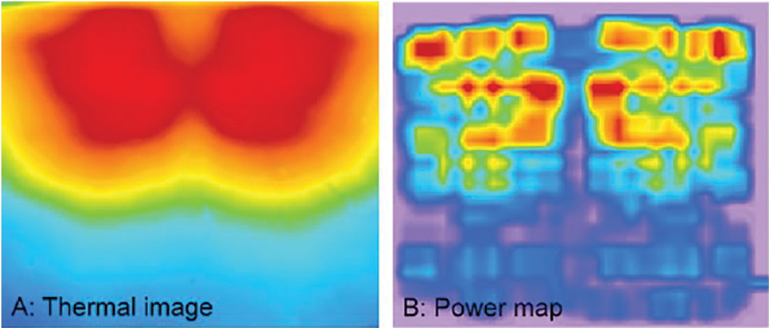
Figure 1: Temperatures and heat source distributions for an IBM PowerPC 970MP® processor
Source: Hamann et al. [30].
Due to the absence of numerical values, it is impossible to provide quantitative information. However, the thermal diffusion effect due to the thermal image obtained in steady state can be observed, such that the definition of the position of the hotspots could only be evaluated using high-end cooling solutions. Also, the only reason for the overlapping effect of the hotspots of this processor not being a major issue is that this specific processor physically separates the position of its cores along with the die, which is not true for most modern processors.
The present study proposes to use the transient response of the microprocessor subject to pulsating heat sources to solve these issues. This minimizes the thermal diffusion occurring during the oscillation of the hotspot temperatures of the processor and thus provides a precise localization of the hotspots for each processor core.
The transient thermal response of a microprocessor has already been explored to characterize and identify hotspots in electronic chips using devices such as a calibrated cooled PIR-fibre (Castellazzi et al. [31]).
However, these applications are not focused on obtaining individual hotspots of each core of a microprocessor using infrared (IR) thermography. Therefore, the acquisition of thermal images of pulsating heat sources of a microprocessor provides an excellent unexplored opportunity, since this technique can provide a maximum spatial resolution between 2–5.5 µm and a response time as fast as milliseconds (Miler [32]), which is sufficient for the desired application.
The basis for the solution of the two-dimensional steady-state inverse heat transfer problem applied to a computer chip is provided by Eq. (1); it consists of the complete heat diffusion equation for a normalized temperature θ containing a heat source term S.
The normalized temperature is defined from a reference temperature, such as:
The steady state solution for this equation consists in neglecting the time-dependent term, such that several discretization methods can be applied to simplify the space derivatives into algebraic expressions. The steady-state discretized heat diffusion equation is adapted from the heat diffusion equation on a processor using a matrix formulation, such as that presented in Cochran et al. [26]:
R denotes the thermal resistances matrix of the microprocessor subject to a heat diffusion condition and e denotes the errors in measurements regarding the temperature distributions used for the representation of this problem.
The advantage obtained by using Eq. (3) to solve the steady-state inverse heat transfer problem consists in obtaining the heat source distribution S using only two parameters obtainable using experimental setups, namely:
• the normalized temperatures distribution θ associated with this specific heat source distribution S;
• the thermal resistances matrix R of the chip.
Regarding the normalized temperature distribution θ of an operating processor, a technique is presented in Amrouch et al. [25]; it consists in using thermoelectric coolers on the opposite surface of the motherboard containing the measured processor to obtain the high heat fluxes required for correctly obtaining the thermal images of the processor. This technique is called Rear-side Thermoelectric-based IR Thermography (RAMA).
Fig. 2, extracted from Amrouch et al. [25], presents a schematic diagram of the experimental setup of this technique. The latter requires the construction of a simple experimental setup, with only air in direct contact with the processor die. Additionally, the upper surface coating of the processor consists of a high emissivity tape, contributing to the low complexity of the setup.
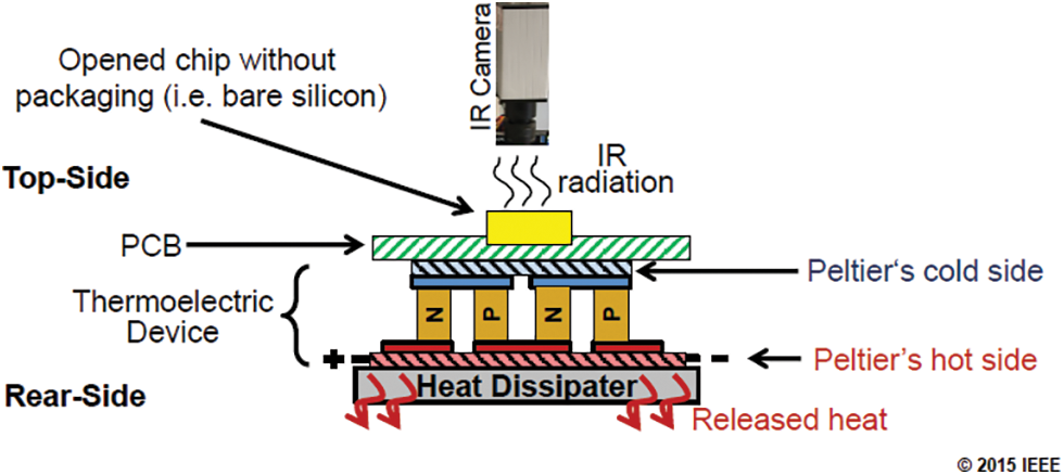
Figure 2: RAMA technique
Source: Amrouch et al. [25].
Regarding the thermal resistance matrix R of the chip, a direct evaluation of Eq. (3) reveals that the application of punctual heat sources to each discretized position of a processor reduces the inverse heat transfer problem to a direct correspondence between the temperatures measured, due to the application of these heat sources and the columns of the thermal resistance matrix R. This evaluation was used in Hamann et al. [24,30] as a preliminary step related to the conversion of the temperature distribution into the heat source distribution of a processor. In these studies, the punctual heat source corresponds to a laser with unitary power applied directly onto a specific position of a test chip.
This experimental setup can be observed in Fig. 3, extracted and adapted from Hamann et al. [30]. The thermal resistance matrix R is obtained considering that each column of this matrix corresponds to the temperature rise of each cell (x,y) of the whole processor, resulting from the laser beam incidence in a specific cell (x,y) of the processor. The incidence of this beam in each cell of the processor provides the full set of columns of the thermal resistance matrix R.
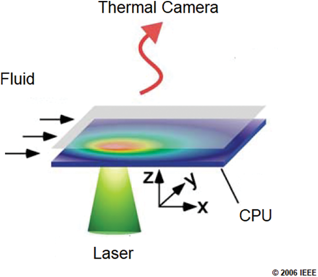
Figure 3: Thermal resistance matrix R: Laser beam experiment
Source: Hamann et al. [30].
However, it must be noted that the steady-state solution of the inverse heat transfer problem presents two major issues regarding the location of the hotspots of a multi-core processor. These problems are addressed in Fig. 4, which presents the thermal image of an INTEL Core 2 Quad Q8400S quad-core microprocessor attached to an ASUS IPM41-D3 motherboard and to a RAMA technique cooling apparatus, subject to a full stress test while running the MICROSOFT Windows 7 Ultimate® operating system.
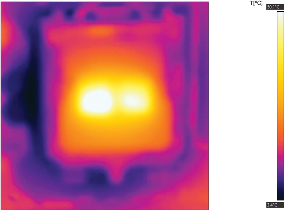
Figure 4: Thermal image: Full stress test of an Intel Core 2 Quad Q8400S
First, it must be noticed that even if this processor separates the cores two-by-two in each of its dies, it is impossible to distinguish the hotspots of individual cores, since the physical proximity and heat diffusion effects homogenize the highest temperatures obtained in the stress test.
Second, this homogenization effect harms the solution of the inverse heat transfer problem by acting as a blurring effect such that the position of the hotspots is masked by the absence of significant thermal gradients between the hotspot and its surroundings.
3 Experimental Setup and Proposed Model
The solution proposed by the present study to overcome these issues consists in using the RAMA technique in a setup similar to the one provided by Amrouch et al. [25]. The experimental setup constructed is presented in the schematic representation of Fig. 5 and consists of a motherboard/processor set without a conventional air heat sink cooled in its lower side by a thermoelectric device (positioned under the motherboard); this, in turn, is cooled by a water cooler whose heat sink is positioned into a box with a mixture containing water and ice. The other computer is used to monitor the temperatures and control the water cooler. A FLIR® i7 compact thermal camera is positioned over the operating microprocessor to obtain its temperature distributions.
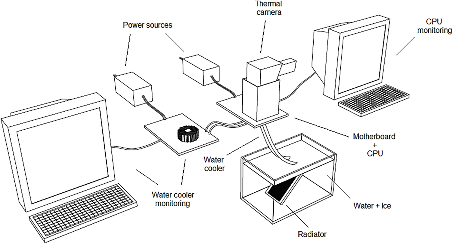
Figure 5: Experimental setup: Schematic representation
As in Amrouch et al. [25], the thermal camera requires the definition of the emissivity of the photographed material. To obtain this parameter, the same technique adopted in Amrouch et al. [25] is used, and black insulating tape with a thickness of 0.13 mm completely covers both the die and the PCB of the microprocessor. The value of 0.92 provided in Griffith et al. [33] is also adopted in the present study. Alternate estimations could be provided using reference plates and infrared thermal cameras using the measurement techniques presented in Yu et al. [34].
However, instead of only executing an idle operating system or a CPU stress test, pulsating instructions are emitted to the microprocessor for each isolated core, resulting in pulsating heat sources. This technique is based on the emission of alternate current excitation pulses provided by Nowroz et al. [35].
This is performed by executing stress tests directly to the other components of the computer, such as the RAM or the hard disk. These tests execute discrete and successive tasks in the microprocessor, resulting in a consequent pulsating behaviour for the heat emitted in this processor due to the execution of these tasks. These pulsating heat sources result in time-dependent temperature fluctuations on the hotspot regions, characterizing a pseudo-transient heat transfer condition in which the hotspot temperature fluctuates between a maximum and a minimum continuously and successively.
For the present study, the intermediate state between these maxima and minima values is important, even if it corresponds to a transient state, since the temperature distributions in these states result in high temperature gradients between the hotspot regions and the rest of the processor, resulting in a clear definition of the position of these regions. Thus, even if this state is not steady, the solution of the inverse heat transfer problem using the temperature distribution provided by this state reveals the hotspot positions with better spatial resolution than a steady-state solution, due to the blurring effect resulting from the thermal diffusion occurring in the steady condition.
The thermal effect obtained by the application of these pulsating instructions can be observed in Fig. 6, which exemplifies how the temperature varies during the execution of a full cycle of one of these instructions performed during a disk test executed by one of the cores of an Intel Core 2 Quad Q8400S microprocessor. This cycle repeats itself with a period of approximately 2 s, so the capture of the thermal images is performed every 0.5 s, providing a full picture of each of the three states presented in Fig. 6, with the intermediate state repeating twice, once during the heating process, and once during the cooling process.
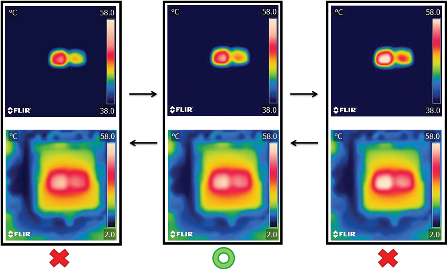
Figure 6: Intel Core 2 Quad Q8400S temperature distributions: Full cycle of pulsating instructions obtained from a disk test
As observed in Fig. 6, the intermediate state presents significantly higher temperature gradients around the hotspot region than the other states. So, even if the true temperature distribution T(x, y, t) and the true power distribution S(x, y, t) are time-dependent, the solution of the steady inverse heat transfer for the frozen picture taken at this intermediate state provides a mean to locate the position of the hotspots of the processor due to the high temperature gradients between these hotspots and the rest of the processor in this state.
These disk tests are performed using the disk test options contained in the software JAM HeavyLoad® and the MICROSOFT Windows Task Manager®, which isolates each core used for the execution of these tests, using the command “Processor Affinity”.
First, the temperature distributions are obtained and subsequently normalized from a reference temperature executing this experimental setup for each processor core. Next, the thermal resistance of the microprocessor is obtained using the experimental procedure presented in Fig. 3 and adopting the hypothesis that the processor studied, as well as all microprocessors of the Core 2 series, can be considered symmetric (Wikibooks [36]), disregarding error e obtained due to the experimental procedures (which has been minimized during these procedures by executing the experiment in a laboratory with a thermally controlled environment and by insulating the region of the microprocessor from radiation, as presented in Fig. 5). The inverse problem resulting from the inversion of Eq. (3) can therefore be solved and reveal the heat source distribution S relative to each temperature distribution obtained from each processor core.
The algorithm used to solve this problem is based on Cochran et al. [26] and constructed using MATLAB® software. This algorithm consists in writing the inverse problem as a minimization problem using a Tikhonov regularization technique, such as:
Thus, regularization parameter α is obtained using the generalized cross-validation method (GCV) and the minimization process is reduced to an algebraic procedure using a decomposition into singular values of the thermal resistance matrix R, such that:
This leads to the calculation of a pseudo-inverse of thermal resistances matrix R as a function of singular decomposition matrices U and V and singular values di of this matrix:
Eq. (6) can obtain heat source distributions S revealing the location of the hotspots of each core of the processor. However, note that the solution of Eq. (6) provides distributions with orders of magnitude that do not correspond to a steady operating processor. Shakouri [1], Bar-Cohen [2] and Iyengar et al. [3] defined as hotspots the regions in which the orders of magnitude of the emitted heat sources are between 500~1000 W/cm²; therefore, the criteria they used cannot be adopted in the present study. Instead, the location of the hotspots is based on the mean heat source gradient between potential hotspots elements and their neighbours, such that the elements considered as hotspots reveal similar mean heat source gradients. This is evaluated by calculating the mean heat source gradients starting from the greatest heat source of each die and descending up to the first non-hotspot element for each core.
The experimental conditions regarding the disk test sending pulsating instructions to each of the four cores are executed and defined as CORE #0, CORE #1, CORE #2, and CORE #3, resulting in the respective intermediate temperature distributions presented in Fig. 7. It can be observed that the maximum temperatures obtained by these thermal images are now concentrated on the hotspots of each processor core and reach values around 54°C for the cores located in the left die, and values between 70°C and 85°C for the cores contained in the right die.
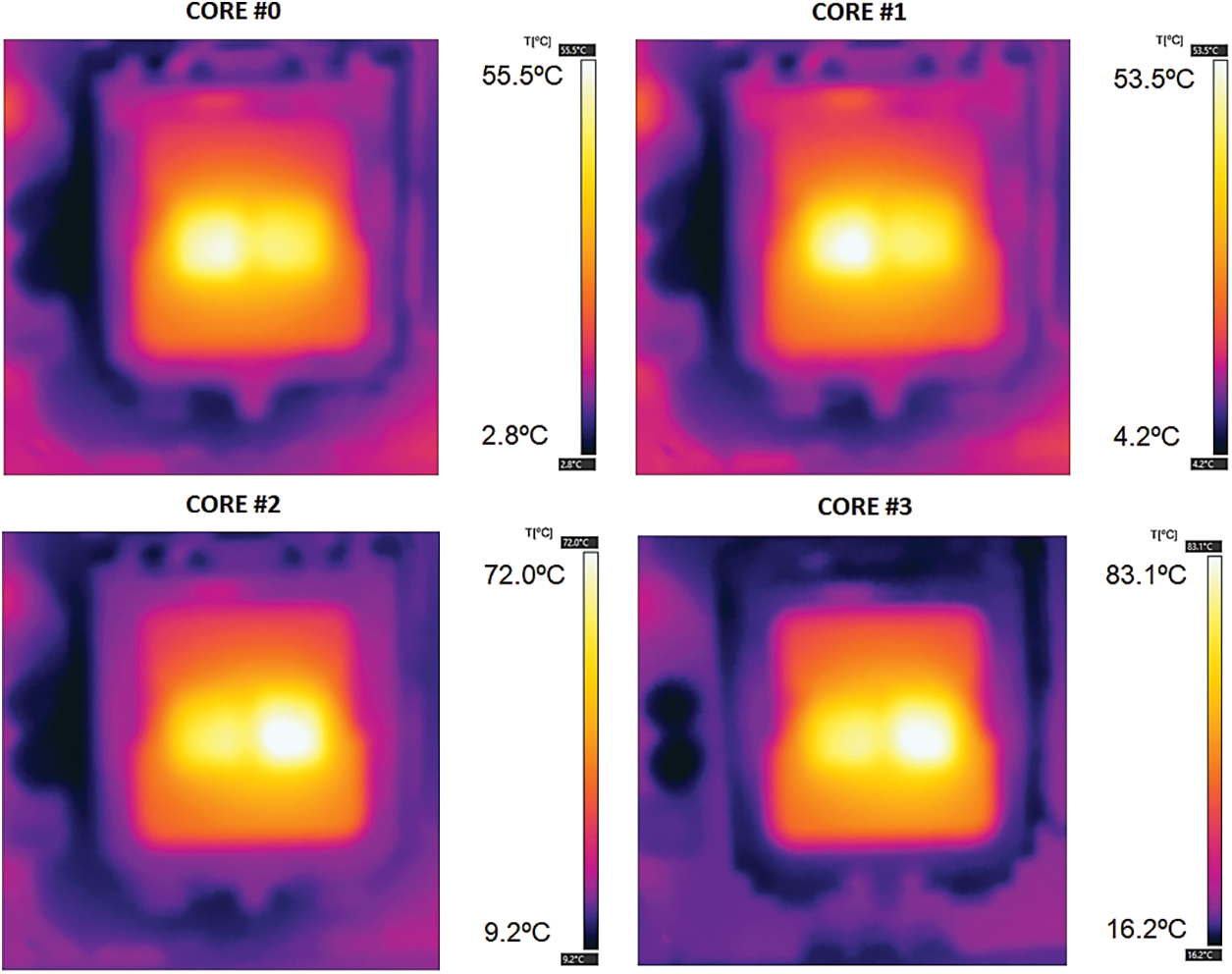
Figure 7: Thermal image: Temperature distributions of each core executing a disk test
The analysis of the qualitative information provided by Fig. 7 suggests that, even if the temperatures obtained reveal an increasing behaviour of the power emitted by each core of the processor, this behaviour occurs due to the accumulation of residual heat due to the sequential execution of the experimental conditions for a significant amount of time, both in the motherboard and in the reservoir containing water and ice. This shows that a few regions of the motherboard were heated with time and stand out in the thermal images from the regions with lower thermal conductivity, such as the motherboard capacitors.
The colours of each temperature distribution presented in Fig. 7 are then converted to grayscale, cut, aligned to Cartesian coordinates using the motherboard capacitors as a reference, and reduced to result in images containing 75 × 75 aligned square elements measuring 0.5 mm × 0.5 mm. Finally, each corresponding reference temperature is adopted as the lower temperatures obtained by the thermal camera and subtracted from each temperature distribution, resulting in the corresponding normalized temperature distributions θ, which are then replotted in Fig. 8.
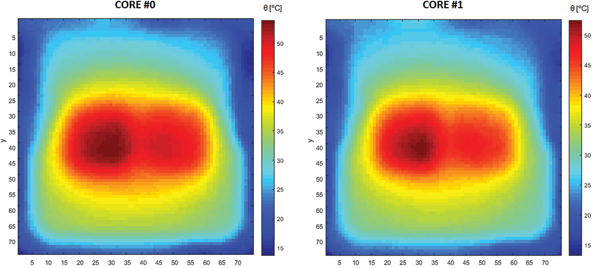
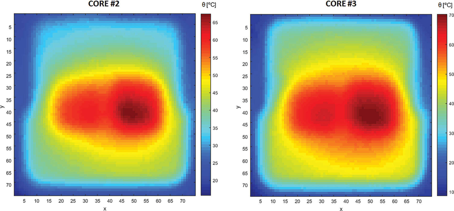
Figure 8: Normalized temperature distributions
The differences regarding the position and the intensity of the hotspots of each core are clearer in Fig. 8, revealing differences regarding the hotspots resulting from cores located in the same die. The hotspots regarding cores 0 and 3 are located nearer to the centre of the die, while the hotspots regarding cores 1 and 2 are closer to the region between the dies.
Therefore, heat source distributions S are obtained for experimental conditions CORE #0, CORE #1, CORE #2, and CORE #3 by the solution of the inverse heat transfer problem. The heat source distribution of an idle condition regarding the execution of only the operating system is also obtained, which is subtracted from these resulting distributions to isolate the effect of the execution of the stress tests. Then, the regions corresponding to the dies containing the stressed cores in each of these experimental conditions are isolated, thus favouring the visualization of the hotspots. The heat source distributions of each of those regions for each core are presented in Fig. 9.
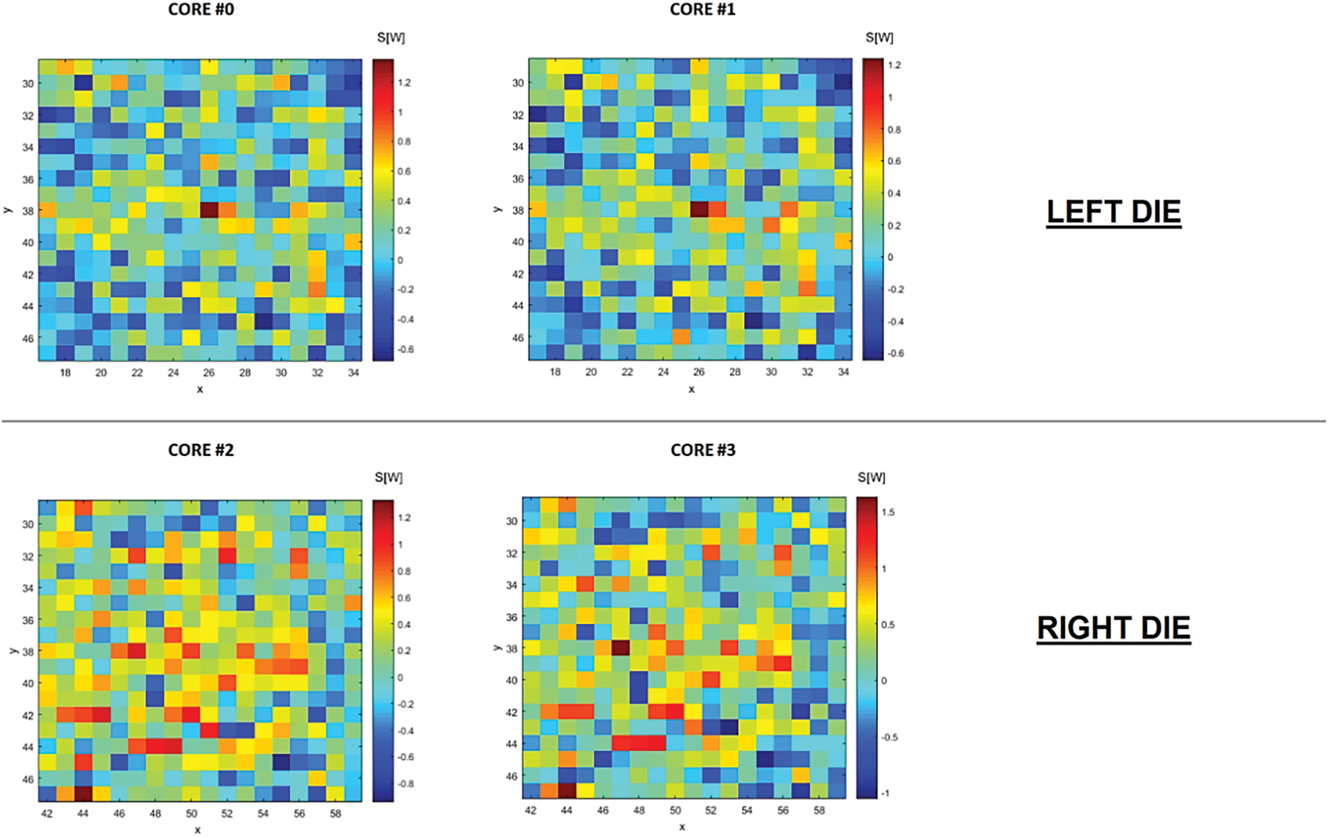
Figure 9: Heat source distributions
Two important aspects obtained in these heat sources must be taken into consideration. First, the unconstrained solution of the inverse heat transfer problem defined in Eq. (4) resulted in heat source distributions containing several negative heat source elements. This is explained due to the unconstrained solution, leading to solutions in which the negative terms compensate for some of the errors obtained in the thermal images, resulting in smoother heat source distributions. However, the quality of this solution is ensured by analysing the solution of the direct heat transfer using the solution obtained for CORE #0, which revealed a mean absolute error between the original temperature distribution and the solution of 0.13°C.
Second, the heat source distributions obtained revealed two clear hotspots, one for each die, that appeared in the stress test of both cores of these dies. The first hotspot is located at the center of the left die, and the second hotspot is in the left lower corner of the right die.
Also, several potential hotspots can be identified on both dies. Due to the unsteady nature of the solutions obtained, the approach of the proposed model is applied to the heat source distributions to reveal each mean heat source gradient between the hottest elements of the distributions and their surroundings. Table 1 summarizes this procedure, in which these gradients were calculated for the well-established hotspots of each die and for the remaining elements in descending order.
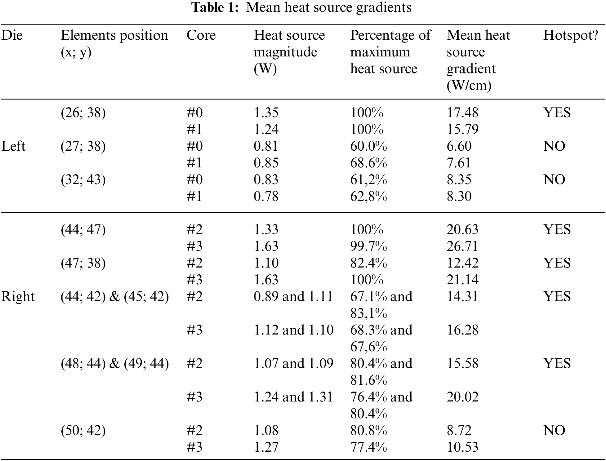
It must first be noticed from Table 1 that a few elements located in the right die revealed heat sources whose magnitudes are considerably close to the heat source magnitude of a neighbour element, with differences such as 0.02 W for the cores revealing the closest gaps. This suggests that these neighbour elements correspond to a singular hotspot whose position is between these two elements, masked by the discretization adopted in the inverse heat transfer solution procedure. Therefore, these elements are gathered for this analysis and, consequently, considered as a single element for calculating the mean heat source gradient, whereby each element serves as a reference for the closer adjacent element for calculating the mean heat source gradient.
The analysis of this table also reveals that in the left die, only the first greatest heat source of this die can be considered as a hotspot for this processor. The next greatest heat sources of this die, in descending order, reveal that their neighbours present mean heat source gradients with values near half the mean heat source gradients found for the first greatest heat source of this die; they are thus not considered hotspots.
Adopting the same criteria, the four greatest heat sources of the right die can be considered as hotspots. The fifth greatest heat source for both cores, corresponding to the element located in the position (50; 42), also reveal mean heat source gradients to its neighbours with values near half the mean heat source gradients found for the greatest heat source of this die, therefore not considered a hotspot, either.
Fig. 10 uses black dots to present the position of all the hotspots obtained previously overlapped to the transparent normalized temperature distribution of the full stress test of the processor presented in Fig. 4. This figure allows to verify that most hotspots are located at positions corresponding to the high temperatures observed in this normalized temperature distribution, corroborating the procedure adopted.
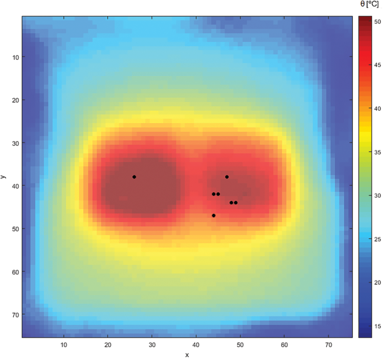
Figure 10: Position of the hotspots
However, it must be pointed out that the greatest hotspot of the right die is located in a position in which the temperature is not as great as the temperature of all the other hotspots of this die. This is explained by the discontinuity of the die in this position; this can lead to the concentration of the heat emitted in this region, even if this element could not be considered a hotspot in terms of the density of operations per second. Hence, when all cores of the processor are stressed, this discontinuity effect is masked by the simultaneous high heat sources occurring all along the processor. This conclusion is supported by comparing Figs. 8 and 9, and observing that much higher temperature gradients are obtained in this region when only COREs #2 or #3 are stressed.
Note that, even with only one hotspot, the left die revealed a wider region with high temperature than the right die. This indicates that the hotspot of the left die is either more intense, and the higher values obtained for the heat sources of the right die in Fig. 8 are a consequence of the accumulation of residual heat in the processor, or its heat is more easily diffused in the left die than in the right die, which contrasts with the symmetry hypothesis adopted in the present study.
The use of the transient response of the microprocessor subjected to pulsating heat sources succeeded in minimizing the effect of thermal diffusion occurring during the operation of a processor. The precise geometrical localization of the hotspots for each processor core could thus be obtained using a thermal camera and the solution of the steady inverse heat transfer problem. Regarding the characterization of the elements of the study, the hotspots, the only major issue encountered could be addressed by using an alternate approach (calculating the mean heat source gradient for each potential hotspot). This revealed that hotspots present similar mean heat source gradients to their neighbour elements.
The adoption of the INTEL Core 2 Quad Q8400S processor as the object of the present study revealed that this processor contains one hotspot located in the centre of its left die and four hotspots located near the lower left corner of its right die, which is consistent with the thermal response obtained both for the stress test applied to each core of this processor and the stress test applied to all of its cores.
Furthermore, the discretization adopted herein for this processor succeeded in providing a suitable way to differentiate the hotspots from its neighbour elements in the y direction, while in the x direction, the results indicated that some heat source elements containing hotspots were located between two elements. Therefore, the element grid should be refined in this direction in future applications.
Finally, future studies should address the minimization of the effects caused by the accumulation of residual heat and by thermal diffusion using this procedure. These effects led to the perception that the hotspots in the right die were more intense than the hotspots in the left die, and this is not observed in the full stress test. Furthermore, additional tests regarding the symmetry hypothesis adopted for the studied processor and the comparison between the density of operations performed and the heat emitted in the border regions of the dies of the processor are promising developments.
Acknowledgement: The authors acknowledge Coordenação de Aperfeiçoamento de Pessoal de Nível Superior (CAPES–Coordination for the Improvement of Higher Education Personnel) for supporting the research.
Funding Statement: The authors received no specific funding for this study.
Author Contributions: The authors confirm contribution to the paper as follows: study conception, design, data collection, analysis, interpretation, results review, writing: Pinto, R. V.; analysis, interpretation, results review and writing review: Fiorelli, F. A. S. All authors reviewed the results and approved the final version of the manuscript.
Availability of Data and Materials: Research data may be obtained upon request to R. V. Pinto (rodrigovidonscky@gmail.com).
Conflicts of Interest: The authors declare that they have no conflicts of interest to report regarding the present study.
References
1. Shakouri, A. (2006). Nanoscale thermal transport and microrefrigerators on a chip. Proceedings of the IEEE, 94(8), 1613–1638.https://doi.org/10.1109/JPROC.2006.879787 [Google Scholar] [CrossRef]
2. Bar-Cohen, A. (2013). Encyclopedia of thermal packaging: A guide to cooling of electronic equipment. USA: World Scientific Publishing Co. Pte. Ltd. [Google Scholar]
3. Iyengar, M., Geisler, K. J. L., Sammakia, B. (2011). Cooling of microelectronic and nanoelectronic equipment. USA: World Scientific Publishing Co. Pte. Ltd. [Google Scholar]
4. Zhao, M., Tian, Y. (2019). Thermal analysis of heat transfer enhancement of rib heat sink for CPU. Frontiers in Heat and Mass Transfer, 13(4), 1–10. https://doi.org/10.5098/hmt.13.4 [Google Scholar] [CrossRef]
5. Tritt, T. M., Subramanian, M. A. (2006). Thermoelectric materials phenomena and applications: A bird’s eye view. MRS Bulletin, 31(3), 188–198. [Google Scholar]
6. Lee, P. S., Garimella, S. V. (2005). Hot-spot thermal management with flow modulation in a microchannel heat sink. ASME 2005 International Mechanical Engineering Congress and Exposition, pp. 643–647. Orlando, FL, USA. https://doi.org/10.1115/IMECE2005-79562 [Google Scholar] [CrossRef]
7. Sharma, C. S., Tiwari, M. K., Zimmermmann, S., Brunschwiler, T., Schlottig, G. et al. (2015). Energy efficient hotspot-targeted embedded liquid cooling of electronics. Applied Energy, 138, 414–422. [Google Scholar]
8. Sharma, C. S., Tiwari, M. K., Poulikakos, D. (2015). A simplified approach to hotspot alleviation in microprocessors. Applied Thermal Engineering, 93, 1314–1323. https://doi.org/10.1016/j.applthermaleng.2015.08.086 [Google Scholar] [CrossRef]
9. Ansari, D., Kim, K. Y. (2018). Hotspot thermal management using a microchannel-pinfin hybrid heat sink. International Journal of Thermal Sciences, 134, 27–39. [Google Scholar]
10. Li, X., Xuan, Y. (2022). Self-adaptive cooling of chips with unevenly distributed high heat fluxes. Applied Thermal Engineering, 202, 117913. https://doi.org/10.1016/j.applthermaleng.2021.117913 [Google Scholar] [CrossRef]
11. Huang, P. S., Chen, Q. C., Huang, C. W., Tsao, S. L. (2014). An efficient thermal estimation scheme for microprocessors. 2014 IEEE 20th International Conference on Embedded and Real-Time Computing Systems and Applications, pp. 1–10. Chongqing,China. https://doi.org/10.1109/RTCSA.2014.6910526 [Google Scholar] [CrossRef]
12. Floros, G., Evmorfopoulos, N., Stamoulis, G. (2019). Efficient IC hotspot thermal analysis via low-rank model order reduction. Integration, 66, 1–8. https://doi.org/10.1016/j.vlsi.2019.02.002 [Google Scholar] [CrossRef]
13. CPU-World (2022). Release dates of desktop microprocessors (2021). https://www.cpu-world.com/Releases/Desktop_CPU_releases_(2021).html (accessed on 05/05/2023) [Google Scholar]
14. Zhang, J., Sadiqbatcha, S., Jin, W., Tan, S. X. D. (2020). Accurate power density map estimation for commercial multi-core microprocessors. 2020 Design, Automation & Test in Europe Conference & Exhibition (DATE), pp. 1085–1090. Grenoble, France. https://doi.org/10.23919/DATE48585.2020.9116545 [Google Scholar] [CrossRef]
15. Zhang, J., Sadiqbatcha, S., O’Dea, M., Amrouch, H., Tan, S. X. D. (2022). Full-chip power density and thermal map characterization for commercial microprocessors under heat sink cooling. IEEE Transactions on Computer-Aided Design of Integrated Circuits and Systems, 41(5), 1453–1466. https://doi.org/10.1109/TCAD.2021.3088081 [Google Scholar] [CrossRef]
16. Sadiqbatcha, S., Zhao, H., Amrouch, H., Henkel, J., Tan, S. X. D. (2019). Hot spot identification and system parameterized thermal modeling for multi-core processors through infrared thermal imaging. 2019 Design, Automation & Test in Europe Conference & Exhibition (DATE), pp. 48–53. Florence, Italy. https://doi.org/10.23919/DATE.2019.8714918 [Google Scholar] [CrossRef]
17. Jin, W., Sadiqbatcha, S., Zhang, J., Tan, S. X. D. (2020). Full-chip thermal map estimation for commercial multi-core CPUs with generative adversarial learning. ICCAD ’20: Proceedings of the 39th International Conference on Computer-Aided Design. Virtual Event, pp. 1–9. USA. https://doi.org/10.1145/3400302.3415764 [Google Scholar] [CrossRef]
18. Sadiqbatcha, S., Zhao, Y., Zhang, J., Amrouch, H., Henkel, J. et al. (2020). Machine learning based online full-chip heatmap estimation. 2020 25th Asia and South Pacific Design Automation Conference (ASP-DAC), pp. 229–234. Beijing, China. https://doi.org/10.1109/ASP-DAC47756.2020.9045204 [Google Scholar] [CrossRef]
19. Sadiqbatcha, S., Zhao, Y., Zhang, J., Amrouch, H., Henkel, J. et al. (2021). Post-silicon heat-source identification and machine-learning-based thermal modeling using infrared thermal imaging. IEEE Transactions on Computer-Aided Design of Integrated Circuits and Systems, 40(4), 694–707. https://doi.org/10.1109/TCAD.2020.3007541 [Google Scholar] [CrossRef]
20. Sadiqbatcha, S., Zhang, J., Amrouch, H., Tan, S. X. D. (2022). Real-time full-chip thermal tracking: A post-silicon, machine learning perspective. IEEE Transactions on Computers, 71(6), 1411–1424. https://doi.org/10.1109/TC.2021.3086112 [Google Scholar] [CrossRef]
21. Lu, J., Zhang, J., Jin, W., Sachdeva, S., Tan, S. X. D. (2023). Learning based spatial power characterization and full-chip power estimation for commercial TPUs. 2023 28th Asia and South Pacific Design Automation Conference (ASP-DAC), pp. 98–103. Tokyo, Japan. [Google Scholar]
22. Xenics Infrared Solutions (2018). Application Note–Thermal Lock-in: Semiconductor Device Analysis. https://www.xenics.com/files/application%20notes/MKT-2018-AN002-R001%20Thermal%20lock-in%20inspection%20of%20semiconductor%20devices%20with%20Xenics%20XCO%20camera%20module.pdf [Google Scholar]
23. Brand, S., Altmann, F. (2019). 3D hot-spot localization by lock-in thermography. In: Microelectronics failure analysis desk reference, pp. 219–227. ASM International. [Google Scholar]
24. Hamann, H. F., Weger, A., Lacey, J. A., Hu, Z., Bose, P. et al. (2007). Hotspot-limited microprocessors: Direct temperature and power distribution measurements. IEEE Journal of Solid-State Circuits, 42(1), 56–64. [Google Scholar]
25. Amrouch, H., Henkel, J. (2015). Lucid infrared thermography of thermally-constrained processors. 2015 IEEE/ACM International Symposium on Low Power Electronics and Design (ISLPED), pp. 347–352. Rome, Italy. https://doi.org/10.1109/ISLPED.2015.7273538 [Google Scholar] [CrossRef]
26. Cochran, R., Nowroz, A. N., Reda, S. (2010). Post-silicon power characterization using thermal infrared emissions. Proceedings of ACM/IEEE Int. Symposium on Low-Power Electronics and Design (ISLPED), Vienna, Austria, pp. 331–336. [Google Scholar]
27. Reda, S. (2011). Thermal and power characterization of real computing devices. IEEE Journal on Emerging and Selected Topics in Circuits and Systems, 1(2), 76–87. https://doi.org/10.1109/JETCAS.2011.2158275 [Google Scholar] [CrossRef]
28. Nowroz, A. N. (2014). Power mapping of computing devices: Fundamentals and applications (Ph.D. Thesis). School of Engineering, Brown University, Providence, RI, USA. [Google Scholar]
29. Pinto, R. V., Fiorelli, F. A. S. (2022). Evaluation of the use of constraints in step-by-step algorithms for the solution of a 2D inverse heat transfer problem. Frontiers in Heat and Mass Transfer, 19(30), 1–10. https://doi.org/10.5098/hmt.19.30 [Google Scholar] [CrossRef]
30. Hamann, H. F., Lacey, J., Weger, A., Wakil, J. (2006). Spatially-resolved imaging of microprocessor power (SIMPHotspots in microprocessors. Proceedings of IEEE ITherm Conference, Las Vegas, USA, pp. 121–125. [Google Scholar]
31. Castellazzi, A., Honsberg-Riedl, M., Wachutka, G. (2006). Thermal characterisation of power devices during transient operation. Microelectronics Journal, 37(2), 145–151. https://doi.org/10.1016/j.mejo.2005.02.123 [Google Scholar] [CrossRef]
32. Miler, J. L. (2012). Limits of hotspot detection and prediction in microprocessors (Ph.D. Thesis). Department of Mechanical Engineering, Stanford University, Stanford, CA, USA. [Google Scholar]
33. Griffith, B. T., Turler, D., Goudey, H. (2002). Infrared thermography. USA: Wiley. [Google Scholar]
34. Yu, H. L., Li, Y. H., Liao, T. Y., Wang, T. C., Tsai, S. F. et al. (2018). Fast and accurate emissivity and absolute temperature maps measurement for integrated circuits. IEEE Transactions on Very Large Scale Integration (VLSI) Systems, 26(5), 912–923. https://doi.org/10.1109/TVLSI.2017.2788437 [Google Scholar] [CrossRef]
35. Nowroz, A. N., Woods, G., Reda, S. (2013). Power mapping of integrated circuits using AC-based thermography. IEEE Transactions on Very Large Scale Integration (VLSI) Systems, 21(8), 1398–1409. https://doi.org/10.1109/TVLSI.2012.2211111 [Google Scholar] [CrossRef]
36. Wikibooks (2022). Microprocessor Design. https://en.wikibooks.org/wiki/Microprocessor_Design (accessed on 05/05/2023) [Google Scholar]
Cite This Article
 Copyright © 2023 The Author(s). Published by Tech Science Press.
This work is licensed under a Creative Commons Attribution 4.0 International License , which permits unrestricted use, distribution, and reproduction in any medium, provided the original work is properly cited.
 Downloads
 Citation Tools