
 Submit a Paper
 Propose a Special lssue
 Open Access
ARTICLE
Study on the Fractal Characteristics of Cavitation Shedding over a Twisted Hydrofoil
1
College of Water Resources and Civil Engineering, China Agricultural University, Beijing, 100083, China
2
Beijing Engineering Research Center of Safety and Energy Saving Technology for Water Supply Network System, China
Agricultural University, Beijing, 100083, China
3
College of Engineering, China Agricultural University, Beijing, 100083, China
* Corresponding Author: Ran Tao. Email:
Frontiers in Heat and Mass Transfer 2023, 21, 161-178. https://doi.org/10.32604/fhmt.2023.041402
Received 21 April 2023; Accepted 15 June 2023; Issue published 30 November 2023
 View Full Text
 Download PDF
Abstract
Cavitation and cavitation erosion often occur and seriously threaten the safe and stable operation of hydraulic machinery. However, during the operation of hydraulic machinery, the cavitation flow field is often difficult to contact and measure, and the shedding and development characteristics of cavitation flow are unknown. This paper uses the Detached Eddy Simulation (DES) turbulence model and Zwart-Gerber-Belamri (ZGB) cavitation model to conduct numerical research on the cavitation flow of a twisted hydrofoil and verifies the effectiveness of numerical simulation by comparing it with experimental results. Then, based on the fractal dimension method, the number and fractal dimension of the main cavitation clusters in two different views are analyzed. The research results show that with the continuous flow of fluid, the cavitation at the tail of the hydrofoil periodically falls off, and the number of cavitation bubbles shows a strong randomness between 1 and 2. The fractal dimension method calculates that the frequency of cavitation bubbles falling off is 30 Hz. The fractal dimension of cavitation also fluctuates periodically. The fractal dimension of cavitation in the side view fluctuates between 1.30–1.38, and the fractal dimension of cavitation in the top view fluctuates between 1.31–1.42. The fractal dimension of the cavitation is closely related to the size and shape of the cavitation. By analyzing the relationship between the cavitation development process and the fractal dimension in the side view, we found the relationship between the development of cavitation in a cycle and the change of fractal dimension, which is of great significance to understanding the characteristics of cavitation flow through the image of the cavitation flow field.Keywords
Nomenclature
| ui | Velocity component |
| t | Time |
| ρ | Density of the working medium |
| ρFi | Mass force |
| p | Pressure term |
| μ | Dynamic viscosity |
| Evaporation source term | |
| Condensation source term | |
| αnuc | Volume fraction |
| Rb | Bubble radius at nucleation position |
| Fvap | Evaporation coefficient of steam |
| Fcond | Condensation coefficient of steam |
| pv | Saturated steam pressure |
| P | Circumference |
| A | Area |
| D | Fractal dimension |
| K | Scale constant |
| Pmin | Minimum pressure on different sections |
| Pin | Average pressure at the inlet of the calculation domain |
| Vin | Average velocity at the inlet of the calculation domain. |
Cavitation and cavitation erosion have always been the key problems that perplex the safe and stable operation of hydraulic machinery. In pumps, hydraulic turbines, and other hydraulic machinery with liquid as the medium, the distribution and variation of the pressure field have always been a concern to researchers [1–3]. This is closely related to the cavitation phenomenon after the pressure drops to the saturation limit. According to a large number of previous studies, cavitation occurs in hydraulic machinery, and the most significant adverse effects include vibration [4], noise [5], performance degradation [6], and material damage [7]. In particular, vibration, noise, and performance degradation are immediate and easy to attract people’s attention. This is closely related to the periodic generation, growth, and collapse of cavitation, and the shock wave and micro-jet caused by cavitation are the key to this series of adverse effects.
Cavitation of bladed hydraulic machinery often occurs on the blade surface. There are several reasons for this. First of all, the liquid flow on the blade surface strikes and separates. There is a local low-pressure region on the blade profile (usually near the leading edge) [8–10]. The pressure in the local zone is often lower than the saturation pressure. Secondly, one of the conditions for vaporization nucleation is that the free energy exceeds the threshold, which is closely related to the surface tension and tensile strength of the nucleus [11]. The tensile strength near the wall is lower than off-wall, and cavitation is easier to be triggered. Thirdly, some blades have poor surface processing with local bulges or pits. The existence of these micro-structures will cause a sharp drop in local pressure and sometimes local cavitation [12,13]. Of course, the factor of blade profile cavitation is the most critical one and is very difficult to avoid. This is because the blade profile is also related to the performance of hydraulic machinery. Changing the blade shape rashly to avoid cavitation will cause significant changes in the performance of the machine [14].
The phenomenon of cavitation and cavitation erosion in hydraulic machinery is widespread and poses a great threat to the safe and stable operation of hydraulic machinery. Monitoring the development characteristics of cavitation and cavitation erosion in hydraulic machinery under continuous working conditions is of great significance for extending the service life of hydraulic machinery and reducing maintenance costs. However, during the operation of hydraulic machinery, the cavitation flow field is often difficult to contact and measure, which brings great difficulties to monitoring the cavitation and erosion characteristics of hydraulic machinery. A large number of scholars have proposed methods for continuously monitoring the cavitation and erosion characteristics of hydraulic machinery through indirect measurement. Al Obaidi et al. [15,16] used vibration technology to detect cavitation phenomena in pumps, and the results showed that when cavitation occurs, the amplitude of the vibration signal is more random and the peak value is higher. Al Obaidi [17] proposed a method for monitoring cavitation characteristics using acoustic analysis techniques based on the inevitable changes in noise in hydraulic machinery caused by cavitation and erosion. The research results show that this method is effective in predicting cavitation in the low-frequency range.
In the above studies, the cavitation characteristics were predicted by using vibration, noise, and other factors, while the cavitation image is the most intuitive performance of cavitation flow, and the research on the prediction of cavitation characteristics by using cavitation image is still less. The cavitation phenomenon (especially the cavitation that causes adverse effects), its shape is complex and broken under the influence of turbulence [18]. When the shedding does not occur, the cavitation cluster is a whole with a non-smooth boundary [19]. When shedding occurs, it will form many isolated elements [20]. Are there any laws in these complex geometric patterns of blade or hydrofoil cavitation? What do these possible laws mean? Are these laws related to hydrodynamics? These questions have always been outstanding, and they may provide new perspectives and ideas for the in-depth analysis of hydraulic machinery cavitation. Since the 1960s, scientists have begun to use fractal geometry to describe geometric objects with irregular and broken shapes [21]. Fractal geometry plays an important role in correlation analysis from the coastline, snowflakes, and biological tissue structures to turbulent flows [22]. Many scientists have proposed turbulence fractal dimension measurement methods, such as Divider method [23], Sausage method [24], Box-Counting method [25]. In the early 1980s, Lovejoy [26] believed that the edge line of tropical clouds could be described by fractal, and applied it to study the fractal dimension of cloud and rain regions. Since then, fractal dimension has been widely used to research the properties of clouds. Inspired by Lovejoy’s work, Batista-Tomás et al. [27–31] conducted a lot of research on cloud morphology using fractal analysis, and found that fractal analysis can be used to predict cyclone movement, which is of great significance to weather prediction. These studies provide a foundation for correlation analysis based on cavitation images.
Based on a twisted hydrofoil with NACA 4-digit as the basic shape [32], this study carried out computational fluid dynamics (CFD) simulation calculation under steady inflow conditions, and compared it with the experimental pressure distribution data and image data. On this basis, the image law of cavitation changing with time is obtained in this study. The number and fractal dimension of the main cavitation clusters in two different 2-dimensional views are obtained by fractal geometric operations, which provides support for the periodic change of cavitation in the case of flow over a hydrofoil.
The fluid flow must follow the basic laws of matter movement, i.e., the conservation of mass, momentum, and energy. Applying these three basic laws to the flow model, three control equations can be obtained, namely, continuity equation, momentum equation, and energy equation. At present, all CFD software simulations are based on the basic control equations of fluid dynamics. In this study, the numerical simulation of the flow around a twisted hydrofoil can be considered as a three-dimensional viscous incompressible turbulent flow. Therefore, the related flow is described by the continuity equation and momentum equation, i.e., Navier-Stokes equation, abbreviated as the N-S equation [33]. In a Cartesian coordinate system, the N-S equation can be written as:
Due to the complexity of turbulent flow and the development level of computers, it is very difficult to use direct numerical solutions for turbulence. To solve this problem, Strelets [34] proposed the detached eddy simulation (DES). DES is a hybrid model of RANS and LES. It uses the RANS method in the boundary layer region and the LES method in the outer layer region. DES overcomes the problem that the LES method has a large amount of computation in the near wall region, and at the same time, it takes advantage of the LES method that has better simulation accuracy for turbulent flow and retains more detailed flow field details. It is the most effective turbulence model for simulating turbulence at present and in the future. The use of the RANS turbulence model or LES turbulence model in DES is determined by the scale of dissipation term, and its formula [35] is:
The selection of the cavitation model is critical to the numerical solution of twisted hydrofoil cavitation [36,37]. A large number of examples show that the Zwart-Gerber-Belamri (ZGB) cavitation model based on the simplified Rayleigh-Plesset (R-P) equation [38] has good simulation accuracy and convergence. It is the most widely used cavitation model at present. Therefore, the ZGB cavitation model is used in this paper to capture the characteristics of two-phase flow caused by cavitation. The ZGB cavitation model mass transport process [35] can be described as:
The dimension of geometric figures is an important feature, and in Euclidean geometry, integers are usually used to describe the dimensions of objects. In Euclidean geometry, straight lines or curves are one-dimensional, planes or spheres are two-dimensional, and objects with length, width, and height are three-dimensional. However, some complex graphics, such as the coastline and Koch curve, are unable to be described by the number of dimensions equal to 1, 2, and 3. The Koch curve is an infinitely long and continuous loop that never intersects itself. The area around the loop is limited and it is smaller than the area of an outer circle. Therefore, the Koch curve squeezed in a limited area with its infinite length, does occupy space. Therefore, its dimension is more than 1 dimension, but less than a 2-dimension graph, that is, its dimension is between 1 and 2, and its dimension is a fraction. The fractal dimension is a noninteger dimension, which is mainly used to measure the effectiveness of the space occupied by complex shapes, and can also reflect the degree of irregularity of these shapes.
There are many methods to calculate the fractal dimension of objects. When studying cavitation phenomena, irregular island-like structures are often encountered, which are called fractal islands. Because these characteristics are suitable for using the area perimeter method to calculate the fractal dimension of the vortex, we choose the fractal dimension based on the perimeter to calculate the fractal dimension of cavitation. To determine the perimeter fractal dimension [39], it needs to be based on the relationship between the perimeter and the area of the fractal island. The mathematical expression for this relationship is as follows:
3 Computing Model and CFD Setup
The research subject of this paper is Delft Twist 11 hydrofoil. The profile of this hydrofoil is NACA0009 hydrofoil with different angles of attack. The thickness yb of NACA0009 hydrofoil changes with chord length c0 as follows [40]:
Initial chord length c0 = 110 mm and maximum thickness hmax = 9.9 mm for NACA0009 hydrofoil. The variation of the angle of attack extension direction of the Delft Twist 11 hydrofoil [41] can be described as:
In this formula, amax = 11° is the maximum angle of attack at the mid-span, the chord length of the hydrofoil L = 150 mm, and the span length S = 300 mm.
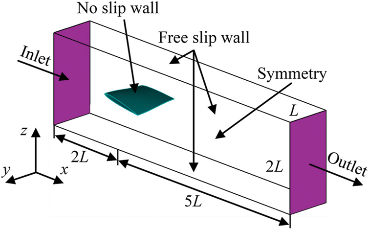
Figure 1: Computational domain schematics of Delft Twist-11 hydrofoil
Grid division is a key step in numerical simulation calculation. The quality and quantity of grid division have a significant influence on the numerical simulation results. The hydrofoil model, which is the research subject of this study, is divided into hexahedron structured grids by ICEM software for the whole watershed of hydrofoil because of its simple structure and to improve the calculation accuracy and save calculation time. First, divide the topological structure according to the geometrical structure of the fluid domain, then divide the hexahedral structure grid, and partially refine the regional grid such as gap and boundary layer. To reduce the influence of grid size on the calculation results, the grid convergence index (GCI) [42] of the Richardson extrapolation method is used to check the grid independence. Based on this method, three sets of grids (N1, N2, and N3) are established in this paper. The total number of grids is 602500, 1394000, 3072400, the value of mesh refinement factor [42] r21 is 1.323, and the value of r32 is 1.301. Then we intercepted three different planes P1, P2, and P3 at 30%, 40%, and 50% span of the hydrofoil along the chord direction, as shown in Fig. 2. In this paper, the minimum pressure on sections P1, P2, and P3 is taken as the index to calculate the independence of the grid. To facilitate parameter comparison, dimensionless treatment of minimum pressure value on hydrofoil surface is carried out with pressure coefficient Cp [43]. The formula is as follows:
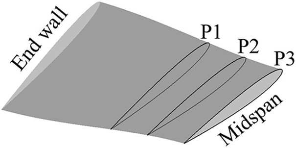
Figure 2: Section position diagram
The change curve of the pressure coefficient with grid size obtained by numerical simulation on different sections is shown in Fig. 3. It can be seen from the figure that the simulated values and Richardson extrapolation values under the three grid scales are relatively close, meeting the grid convergence conditions, indicating that the grid has good independence. Considering the calculation accuracy and speed comprehensively, the second set of grids with 1394000 grid nodes is selected as the final grid scheme in the subsequent analysis, and the grid partition diagram is shown in Fig. 4.
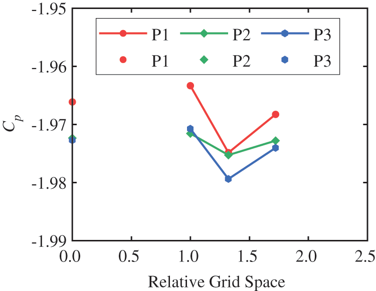
Figure 3: The variation of Cp with grid size and Richardson extrapolation value on different sections
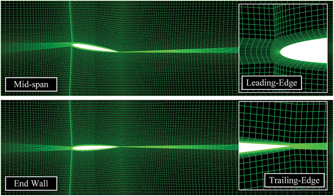
Figure 4: Grid dividing schematics
In this paper, commercial software ANSYS CFX is used for numerical simulation and the DES model is used for the turbulence model. The calculation medium is pure water and water vapor at 25°C. The reference pressure in the calculation domain is set to a standard atmospheric pressure and the critical cavitation pressure is set to 3100 Pa. The boundary of the computational domain is mainly set as follows:
(1) The inlet of the calculation domain is set as the inlet of flow rate, the equation for inlet conditions is Vin = 6.97 m/s and
(2) The static pressure boundary is used at the outlet of the computational domain, the equation for outlet conditions is P = 29160 Pa and
(3) The hydrofoil surface is set as the no-slip wall, and the upper and lower surfaces in the calculation domain and the end wall of the hydrofoil are set as the free-slip wall. To reduce the calculation, the hydrofoil is cut in the middle and the middle section is set as the symmetrical plane.
The numerical simulation of twisted hydrofoil cavitation first carries out the steady calculation. RMS residual of steady calculation is set as 10−6, and the maximum iterative steps are 1000. The unsteady calculation is founded on the calculation results of the steady calculation. The total time for unsteady calculation is set to 0.1 s, and each time step is 0.0001 s. The maximum number of iterations for each time step is 10. The convergence criterion is RMS = 1.0 × 10⁻⁵.
4 Validation of Numericcxal Simulation
In order to verify the validity of the numerical simulation results, the pressure distributions on sections P1, P2, and P3 are compared with the experimental results. The experimental results are available from Delft University of Technology (Delft) [44] and École Polytechnique Fédérale de Lausanne (EPFL) [45]. Fig. 5 shows the comparison between numerical simulation results in different planes and the two experimental results. It can be seen from the diagram that the numerical simulation results agree well with the EPFL experimental results on different sections. The numerical simulation results differ greatly from Delft experimental results at very individual points, but the overall pressure distribution is basically the same. Therefore, the numerical simulation results based on the settings of the calculation conditions in this paper can effectively reflect the true situation of twisted hydrofoil flow.
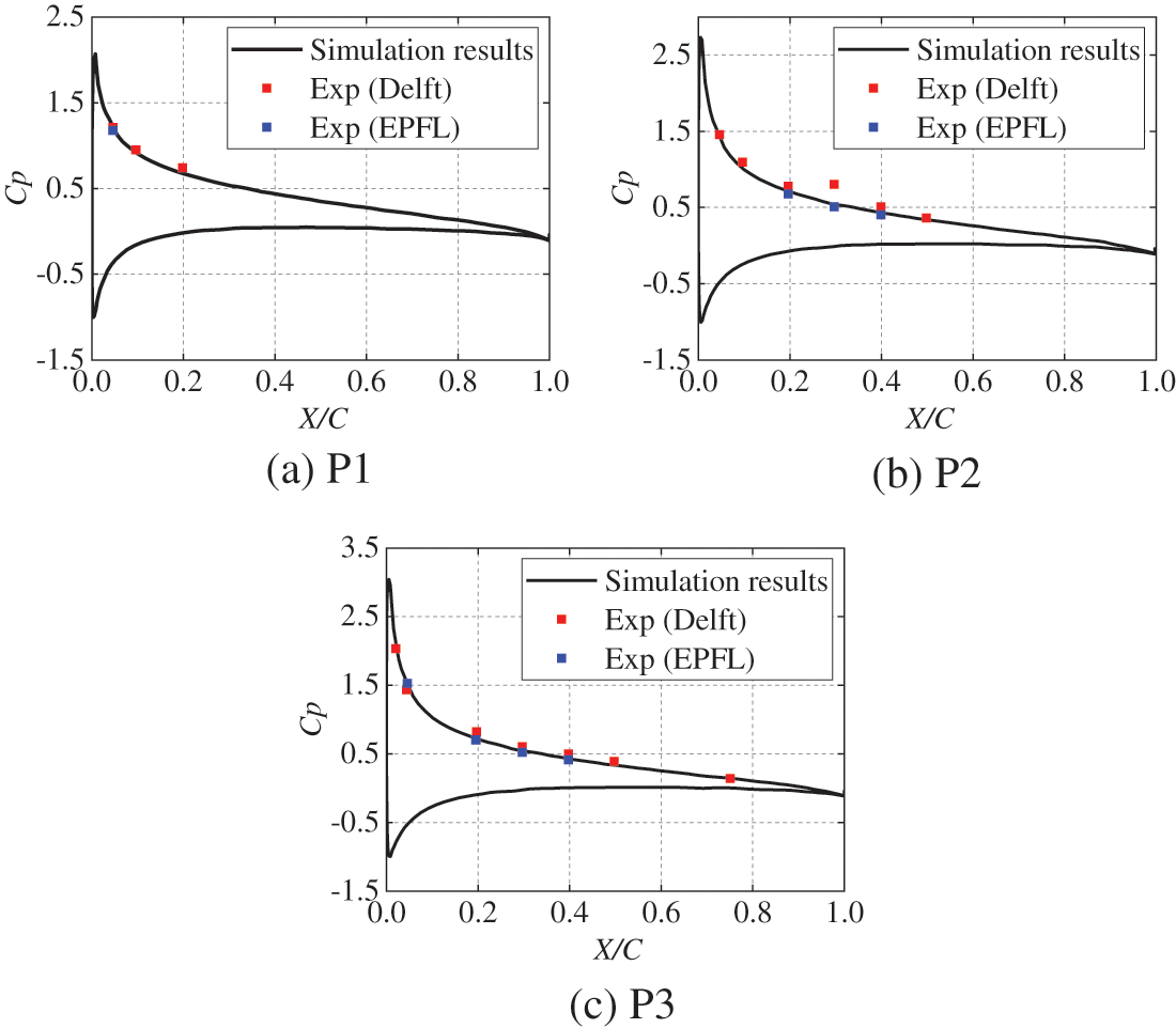
Figure 5: Comparisons of pressure distribution with experimental results at different hydrofoil spanwise positions
The pressure nephogram shown in Fig. 6 can be obtained by dimensionless the pressure on the three sections P1, P2, and P3 with the dimensionless coefficient Cp. It can be seen from the figurethat the pressure distribution is basically the same at different sections, the pressure changes greatly near the airfoil, and the pressure remains unchanged at other parts. The pressure on the upper surface of the hydrofoil is low, and the range of the low-pressure zone is mainly concentrated on the first half of the airfoil. The pressure on the lower surface of the hydrofoil is high, and the high-pressure zone is mainly concentrated on the airfoil head. In addition, the size of the low-pressure zone is significantly larger than the high-pressure zone.
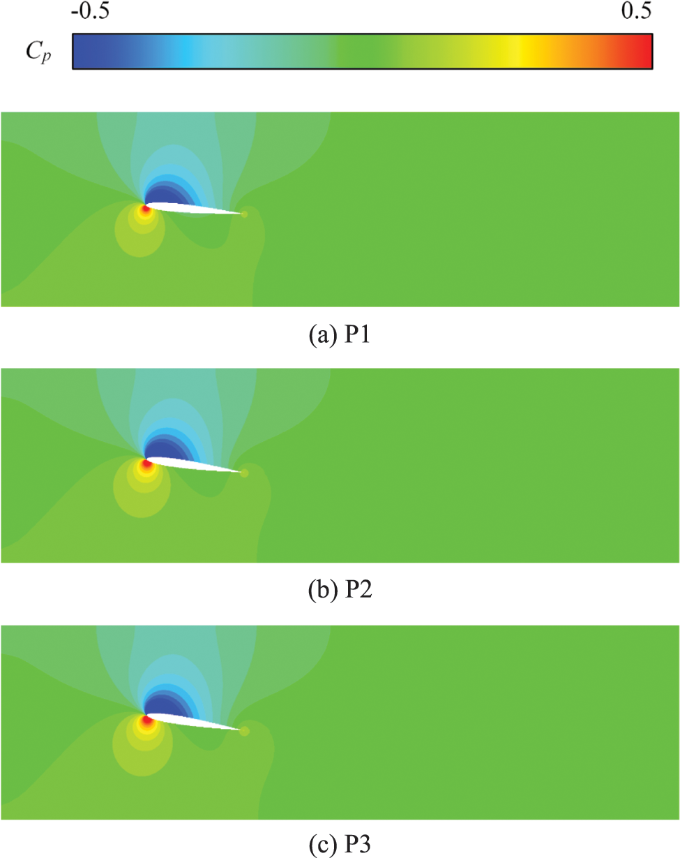
Figure 6: Pressure nephogram of different hydrofoil spanwise positions
The velocity nephogram shown in Fig. 7 can be obtained by dimensionless the velocity on the three sections P1, P2, and P3 with the velocity coefficient Cv = V/Vin. It can be seen that the velocity distribution is basically the same for the three sections. Due to the influence of the hydrofoil on the flow, the flow velocity on the upper surface of the hydrofoil is larger, and the flow velocity on the lower surface of the hydrofoil is smaller. Similar to the pressure distribution, the higher velocity region on the upper surface of the hydrofoil is also significantly greater than the lower velocity region on the lower surface of the hydrofoil. There is a long strip of the first velocity region at the tail of the hydrofoil, and the length of the low-velocity region varies with different sections.
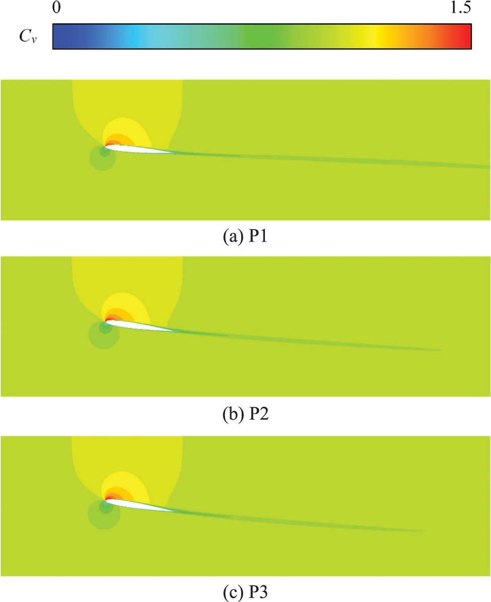
Figure 7: Pressure nephogram of different hydrofoil spanwise positions
In order to further verify the effectiveness of the numerical simulation, this paper selects the equivalent of cavitation volume fraction av = 0.01 to visualize the cavitation phenomenon obtained from the numerical simulation. Fig. 8 shows the qualitative comparison between the captured cavitation shedding cycle and the numerical simulation. It can be seen from the comparison between the experimental results and the numerical simulation results that there are some differences in the cavitation length during the cavitation shedding cycle. This may be due to the fact that the cavitation shedding process is a random process and there are some differences in the development process of bubbles in each cavitation shedding cycle, this difference also exists in Melissaris et al. [41] study. Overall, the cavitation images obtained from experiments and numerical simulations at different stages are basically consistent, and the numerical simulation results are effective.
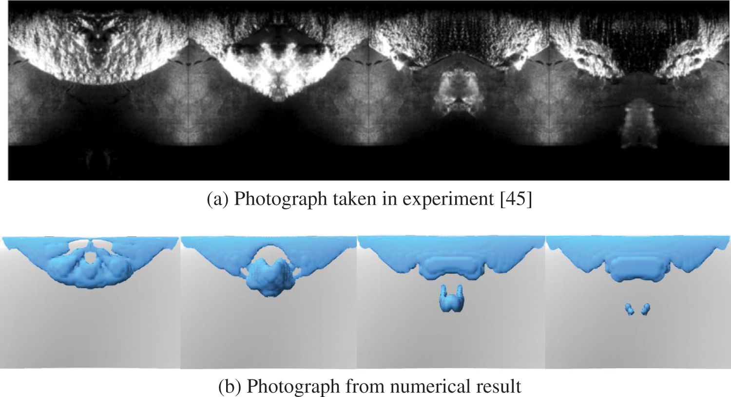
Figure 8: Comparison of experimental and simulated results of cavitation shedding cycle
From the figure, we can see the four stages of cavity shedding in twisted hydrofoils. In the first stage, free bubbles caused by twisted hydrofoils accumulate in the middle of the leading edge of the hydrofoil to form stable sheet cavitation. In the second stage, the cavity in the middle of the sheet cavitation is torn and shows a tendency to detach. In the third stage, the tail cavitation detaches from the sheet cavitation, and the detached cavity gradually transports downstream. In the fourth stage, the falling bubbles gradually shrink and eventually disappear. The cavity shedding cycle simulated by the DES turbulence model in this article is basically consistent with the research results of Ji et al. [46] using the PANS method.
In this paper, the cavitation volume fraction av = 0.01 is used to display the bubbles at different flow moments, and the bubble images at different flow times are obtained through the side view and top view. Fig. 9 is a schematic diagram of the cavitation two-dimensional image processing process obtained from the top view at a certain time. The specific operation is to binarize the bubble image first and change the gray value of each pixel in the image to 0 or 255; Then morphological operations are carried out to remove the small bubbles in the image and keep the shape and position of the main bubbles unchanged. Finally, mark the bubbles, mark each bubble in the image with red numbers, get the number of bubbles in each image, and calculate the circumference and area of each bubble to prepare for the subsequent calculation of the fractal dimension of each bubble and its analysis [47].
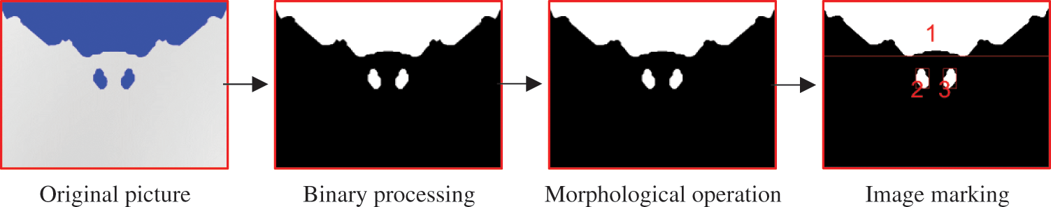
Figure 9: Image processing process
5.2 Time Evolution of Bubble Fractal Characteristics
In this paper, the side view and top view of twisted hydrofoil cavitation are obtained at the time interval of 0.001 s and processes the images at each time using the above image processing process to obtain the evolution process of the number of bubbles and fractal dimension with time.
Fig. 10a shows the change curve of the number of bubbles with time after processing the bubble image in the top view. It can be seen from the figure that the number of bubbles in the top view is between 1 and 3. Among them, the flaky bubble in the middle of the leading edge of the hydrofoil always exists. The flaky bubble periodically produces the tail bubble and the generation and collapse of the tail bubble cycle. The number of falling bubbles has a strong randomness. Sometimes one bubble falls off, and the falling bubbles decompose into two bubbles after a certain time; Sometimes two bubbles fall off directly. In order to better understand the frequency of bubble generation and collapse, this paper uses Fourier transform to obtain the frequency domain image shown in Fig. 10b. From the frequency domain image of the number of bubbles, it can be found that the main frequencies are 30, 60, and 85 Hz, and the frequency of bubble generation and collapse is 30 Hz. The difference between the predicted results and the 32.2 Hz obtained in the experiment [45] is only 7%, which is consistent with the bubble shedding frequency 30 Hz simulated by Bensow [48] using the DES turbulence model in 2011, indicating that the image analysis method based on fractal dimension is effective in predicting cavitation characteristics.
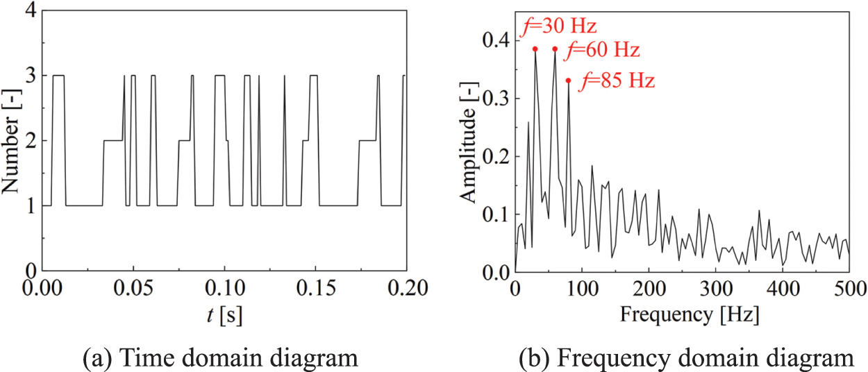
Figure 10: Time domain and frequency domain diagram of the number of bubbles in the top view
Fig. 11a shows the change curve of the fractal dimension of flaky bubbles with time after processing the bubble image in the top view. It can be seen from the figure that the fractal dimension of the flaky bubbles in the top view fluctuates between 1.31–1.42. In order to intuitively compare the relationship between fractal dimension and bubble shape, we select the bubble images at the peak and trough to compare. By comparing these two images, we can find that when the fractal dimension is small, the cavitation state of the twisted hydrofoil is in the fourth stage of the cavity-shedding cycle, and when the fractal dimension is large, the cavitation state of the twisted hydrofoil is in the second stage of the cavity shedding cycle. To some extent, the fractal dimension is also related to the size and shape of the bubbles. Fig. 11b is the frequency domain diagram obtained by the Fourier transform in Fig. 11a. From the fractal dimension frequency domain diagram of the flaky bubbles in the top view, it can be found that the main frequency is 30 Hz. Compared with the frequency domain diagram of the number of bubbles, the frequency domain diagram of fractal dimension can reduce the interference of noise signals and more accurately locate the frequency of bubble generation and collapse.
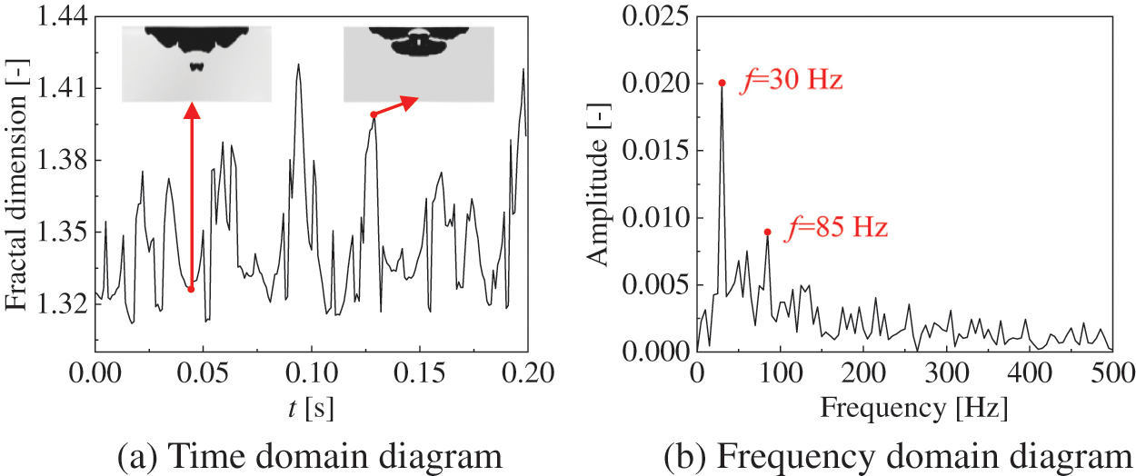
Figure 11: Time domain and frequency domain diagram of fractal dimension of bubbles in the top view
Fig. 12a shows the change curve of the number of bubbles with time after processing the cavitation image in the side view. It can be seen from the figure that the number of bubbles in the side view is the same as that in the top view, both between 1 and 3. However, the number of images with a cavitation number of 3 observed in the side view is significantly smaller than that in the top view. This is because the flow direction of the tail bubbles that fall off from the hydrofoil flaky bubbles has a small difference, so that two tail bubbles overlap in the side view, so only one tail bubble can be observed. In order to more intuitively analyze the frequency of the periodic shedding of tail bubbles, we use Fourier transform to obtain the frequency domain diagram shown in Fig. 12b. It can be seen from the figure that the main frequencies in the frequency domain diagram are 30, 60, and 80 Hz, which are basically the same as those in the frequency domain diagram of the number of bubbles in the top view of Fig. 10b.
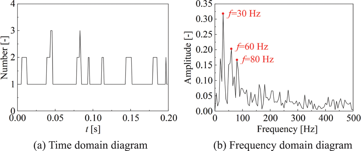
Figure 12: Time domain and frequency domain diagram of the number of bubbles in the side view
Fig. 13a shows the change curve of the fractal dimension of the flaky bubbles with time after the processing of the cavitation image in the side view. It can be seen from the figure that the fractal dimension of bubbles in the side view shows obvious periodicity with time, and fluctuates between 1.30–1.38. Similar to the analysis of the top view, we selected the bubble images at the peak and trough in the side view for comparison. Through comparison and analysis, we found that when the bubble image is completely filled, the fractal dimension of the bubble is small; On the contrary, the fractal dimension is larger. Fig. 13b is the frequency domain diagram obtained by the Fourier transform in Fig. 13a. It can be seen from the figure that the main frequencies in Fig. 11b are 30 and 60 Hz, which are similar to the experimental results.
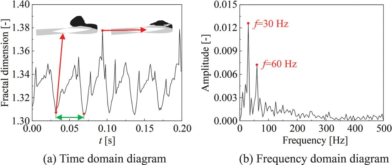
Figure 13: Time domain and frequency domain diagram of fractal dimension of bubbles in the side view
Since the change of fractal dimension with time in the side view shows a good periodicity, we select a period represented by the green arrow in Fig. 13a to analyze the development process of cavitation. The start and end times of the cycle are 0.032 and 0.069 s, respectively. We take a cavitation image every 0.001 s, a total of 38 cavitation images as shown in Fig. 14. By comparing the change of cavitation image and fractal dimension with time, the complete period of cavitation shedding can be described as follows: when the cavitation of the hydrofoil tail is maximum, the fractal dimension of the cavitation image reaches the minimum value of 1.31. Then with the separation and collapse of the tail cavity and the sheet cavity and the continuous development of the sheet cavity, the fractal dimension of the cavity gradually increases. When there is a tail cavity in the cavity to be generated, the fractal dimension reaches the maximum value of 1.35. Finally, with the increase of the tail cavity, the fractal dimension decreases. When the tail cavity increases to the maximum, the fractal dimension of the cavity reaches the minimum.
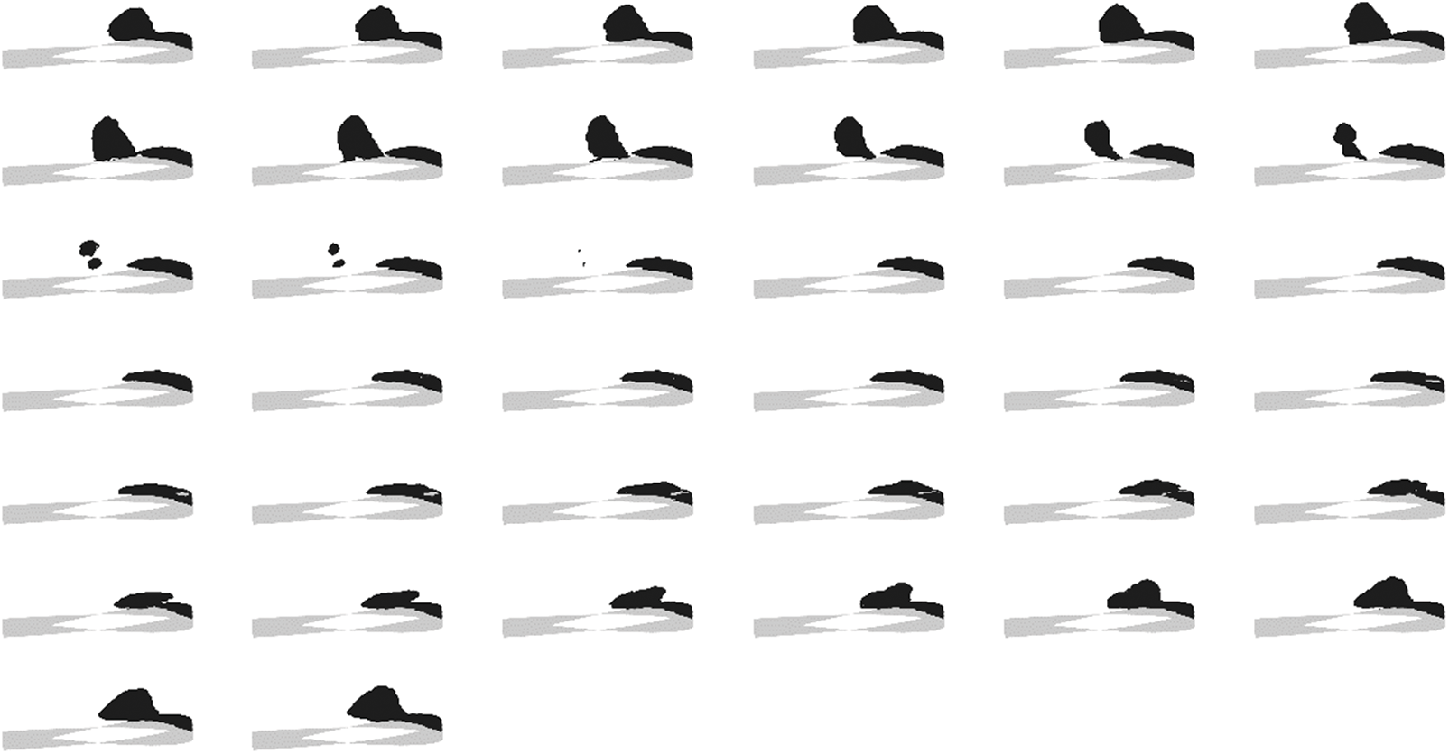
Figure 14: Cavitation image in one cycle
Based on numerical simulation, this paper uses the fractal dimension method to study the cavitation shedding phenomenon caused by twisted hydrofoil. The conclusion can be drawn as the following two points:
(1) It is found that the cavitation shedding caused by twisted hydrofoil shows obvious periodicity. The predicted frequency of bubble shedding through image processing is 30 Hz, which is only 7% different from the experimental results, indicating the effectiveness of using image processing methods to predict cavitation characteristics. The number of falling bubbles has a strong randomness. Sometimes one bubble falls off, and the falling bubbles decompose into two bubbles after a certain time; Sometimes two bubbles fall off directly. On the whole, the number of falling bubbles is between 1 and 2.
(2) Under two different observation angles, the fractal dimension of the twisted hydrofoil cavitation image also fluctuates periodically. The fractal dimension of cavitation in the side view fluctuates between 1.30–1.38, and the fractal dimension of cavitation in the top view fluctuates between 1.31–1.42. The fractal dimension of the cavitation is closely related to the size and shape of the cavitation.
(3) Using the change of fractal dimension in the side view, we can describe the complete period of cavitation shedding as follows: when the cavitation at the tail of the hydrofoil is the largest, the fractal dimension of the cavitation is the smallest; Secondly, with the separation and collapse of the tail bubble and the development of the flaky bubble, the fractal dimension of the bubble increases gradually; Then, with the continuous development of the flaky cavitation, when the tail cavitation is about to occur, the fractal dimension reaches the maximum value; Finally, with the increasing of the tail bubble, the fractal dimension of the bubble decreases. When the tail bubble increases to the maximum, the fractal dimension of the bubble reaches the minimum again.
Based on the image analysis method, this study reveals the relationship between the periodic change of cavitation and the change of fractal dimension in the case of hydrofoil flow, providing a theoretical basis for predicting the occurrence and development of cavitation. Based on the conclusions of this study, when the cavitation flow field is not easy to contact and measure, the results of image measurement can also provide significant conclusions. This provides the possibility to expand the research methods and means of cavitation.
In this paper, the image processing method based on fractal dimension is applied to analyze the cavitation phenomenon of twisted hydrofoil, and the relationship between the periodic development of cavitation and the change of fractal dimension is found. However, cavitation characteristics include many aspects. In the subsequent research, we can continue to explore the relationship between fractal dimension and other characteristics of cavitation, and further explore the value of this image-processing method for predicting cavitation characteristics. In addition, this article only discusses the cavitation phenomenon of a twisted hydrofoil, but there are significant differences in cavitation phenomena between different hydrofoils and rotating blades, and the conclusions of this article may not be applicable to a large number of studies. Therefore, in subsequent research, we can apply this method to analyze the cavitation phenomenon of different research objects. Through a large number of examples, we can find the similarities of this method in analyzing cavitation phenomena and obtain conclusions that can be applicable to most situations.
Acknowledgement: The authors would like to acknowledge the National Natural Science Foundation of China for its support in the present study.
Funding Statement: This work is supported by the National Natural Science Foundation of China, Grant No. 51909131.
Author Contributions: The authors confirm contribution to the paper as follows: study conception and design: Ruofu Xiao, Ran Tao; data collection: Zilong Hu, Weilong Guang; analysis and interpretation of results: Ran Tao, Di Zhu; draft manuscript preparation: Zilong Hu, Weilong Guang. All authors reviewed the results and approved the final version of the manuscript.
Availability of Data and Materials: The data are available when requested.
Conflicts of Interest: The authors declare that they have no conflicts of interest to report regarding the present study.
References
1. Benigni, H. (2020). Cavitation in hydraulic machines: Measurement, numerical simulation and damage patterns. American Society of Mechanical Engineers Digital Collection, 83716, V001T01A010. [Google Scholar]
2. Al-Obaidi, A. R., Mohammed, A. A. (2019). Numerical investigations of transient flow characteristic in axial flow pump and pressure fluctuation analysis based on the CFD technique. Journal of Engineering Science & Technology Review, 12(6), 70–79. [Google Scholar]
3. Ramadhan Al-Obaidi, A. (2019). Numerical investigation of flow field behaviour and pressure fluctuations within an axial flow pump under transient flow pattern based on CFD analysis method. Journal of Physics: Conference Series, 1279, 012069. [Google Scholar]
4. Al-Obaidi, A. R. (2020). Detection of cavitation phenomenon within a centrifugal pump based on vibration analysis technique in both time and frequency domains. Experimental Techniques, 44(3), 329–347. [Google Scholar]
5. Chudina, M. (2003). Noise as an indicator of cavitation in a centrifugal pump. Acoustical Physics, 49(4), 463–474. [Google Scholar]
6. Al-Obaidi, A. R. (2020). Influence of guide vanes on the flow fields and performance of axial pump under unsteady flow conditions: Numerical study. Journal of Mechanical Engineering and Sciences, 14(2),6570–6593. [Google Scholar]
7. Benigni, H. (2020). Cavitation in hydraulic machines: Measurement, numerical simulation anddamage patterns. Proceedings of The ASME 2020 Fluids Engineering Division Summer Meeting, V001T01A010. New York, USA. [Google Scholar]
8. Tao, R., Li, P., Yao, Z., Xiao, R. (2022). Investigation of the flow energy dissipation law in a centrifugal impeller in pump mode. Proceedings of the Institution of Mechanical Engineers, Part A: Journal of Power and Energy, 236(2), 260–272. [Google Scholar]
9. Zhu, D., Xiao, R., Liu, W. (2021). Influence of leading-edge cavitation on impeller blade axial force in the pump mode of reversible pump-turbine. Renewable Energy, 163(4), 939–949. [Google Scholar]
10. Al-Obaidi, A. R. (2021). Analysis of the effect of various impeller blade angles on characteristic of the axial pump with pressure fluctuations based on time-and frequency-domain investigations. Iranian Journal of Science and Technology, Transactions of Mechanical Engineering, 45(2), 441–459. [Google Scholar]
11. Mahmud, K. (2020). A molecular scale study of cavitation growth and shock response in soft materials (Ph.D. Thesis). University of Texas, Arlington. [Google Scholar]
12. Zhuang, D. D., Zhang, S. H., Liu, H. X., Chen, J. (2022). Cavitation erosion behaviors and damage mechanism of Ti-Ni alloy impacted by water jet with different standoff distances. Engineering Failure Analysis, 139(4), 106458. [Google Scholar]
13. Gu, Y., Yu, L., Mou, J., Shi, Z., Yan, M. et al. (2022). Influence of circular non-smooth structure on cavitation damage characteristics of centrifugal pump. Journal of the Brazilian Society of Mechanical Sciences and Engineering, 44(4), 155. [Google Scholar]
14. Iwai, Y. (2000). Hydraulic machinery. Cavitation of Hydraulic Machinery, 1, 269. [Google Scholar]
15. Al-Obaidi, A. R., Mishra, R. (2020). Experimental investigation of the effect of air injection on performance and detection of cavitation in the centrifugal pump based on vibration technique. Arabian Journal for Science and Engineering, 45(7), 5657–5671. [Google Scholar]
16. Al-Obaidi, A. R. (2020). Experimental comparative investigations to evaluate cavitation conditions within a centrifugal pump based on vibration and acoustic analyses techniques. Archives of Acoustics, 45(3),541–556. [Google Scholar]
17. Al-Obaidi, A. (2020). Experimental investigation of cavitation characteristics within a centrifugal pump based on acoustic analysis technique. International Journal of Fluid Mechanics Research, 47(6), 501–515. [Google Scholar]
18. Long, X., Cheng, H., Ji, B., Arndt, R. E., Peng, X. (2018). Large eddy simulation and Euler-Lagrangian coupling investigation of the transient cavitating turbulent flow around a twisted hydrofoil. International Journal of Multiphase Flow, 100(1), 41–56. [Google Scholar]
19. Liu, H., Lin, P., Tang, F., Chen, Y., Zhang, W. et al. (2021). Experimental study on the relationship between cavitation and lift fluctuations of S-shaped hydrofoil. Frontiers in Energy Research, 9, 813355. [Google Scholar]
20. Liu, J., Yu, J., Yang, Z., He, Z., Yuan, K. et al. (2021). Numerical investigation of shedding dynamics of cloud cavitation around 3D hydrofoil using different turbulence models. European Journal of Mechanics-B/Fluids, 85, 232–244. [Google Scholar]
21. Mandelbrot, B. B., Mandelbrot, B. B. (1982). The fractal geometry of nature. New York: WH Freeman. [Google Scholar]
22. Seo, Y., Ko, H. S., Son, S. (2020). The effect of nozzle geometry on the turbulence evolution in an axisymmetric jet flow: A focus on fractals. Physica A: Statistical Mechanics and Its Applications, 550(13), 124145. [Google Scholar]
23. Xu, H. X., Wang, G. M., Liang, J. G., Zhang, C. X., Wu, F. T. (2012). Modelling of composite right/left-handed transmission line based on fractal geometry with application to power divider. IET Microwaves, Antennas & Propagation, 6(13), 1415–1421. [Google Scholar]
24. Takeno, T., Murayama, M., Tanida, Y. (1990). Fractal analysis of turbulent premixed flame surface. Experiments in Fluids, 10(2–3), 61–70. [Google Scholar]
25. Perret, J. S., Prasher, S. O., Kacimov, A. R. (2003). Mass fractal dimension of soil macropores using computed tomography: From the box-counting to the cube-counting algorithm. European Journal of Soil Science, 54(3), 569–579. [Google Scholar]
26. Lovejoy, S. (1982). Area-perimeter relation for rain and cloud areas. Science, 216(4542), 185–187. [Google Scholar] [PubMed]
27. Batista-Tomás, A. R., Díaz, O., Batista-Leyva, A. J., Altshuler, E. (2016). Classification and dynamics of tropical clouds by their fractal dimension. Quarterly Journal of the Royal Meteorological Society, 142(695), 983–988. [Google Scholar]
28. Sánchez, N., Alfaro, E. J., Pérez, E. (2005). The fractal dimension of projected clouds. The Astrophysical Journal, 625(2), 849. [Google Scholar]
29. Luo, Z., Wang, Y., Ma, G., Yu, H., Wang, X. et al. (2014). Possible causes of the variation in fractal dimension of the perimeter during the tropical cyclone Dan motion. Science China Earth Sciences, 57(6), 1383–1392. [Google Scholar]
30. von Savigny, C., Brinkhoff, L. A., Bailey, S. M., Randall, C. E., Russell III, J. M. (2011). First determination of the fractal perimeter dimension of noctilucent clouds. Geophysical Research Letters, 38(2), L02806. [Google Scholar]
31. Brinkhoff, L. A., von Savigny, C., Randall, C. E., Burrows, J. P. (2015). The fractal perimeter dimension of noctilucent clouds: Sensitivity analysis of the area-perimeter method and results on the seasonal and hemispheric dependence of the fractal dimension. Journal of Atmospheric and Solar-Terrestrial Physics, 127(1), 66–72. [Google Scholar]
32. Hoekstra, M., van Terwisga, T., Foeth, E. J. (2011). Smp11 workshop-case 1: Delftfoil. Proceedings of the 2nd International Symposium on Marine Propulsors, Hamburg, Germany. [Google Scholar]
33. Anderson, J. D., Wendt, J. (1995). Computational fluid dynamics. New York: McGraw-Hill. [Google Scholar]
34. Strelets, M. (2001). Detached eddy simulation of massively separated flows. 39th Aerospace Sciences Meeting and Exhibit. Reno, USA. [Google Scholar]
35. Xu, B., Liu, K., Deng, J., Liu, X., Shen, X. et al. (2023). Thermodynamic effect on attached cavitation and cavitation-turbulence interaction around a hydrofoil. Ocean Engineering, 281(6), 114764. [Google Scholar]
36. Cheng, H., Long, X., Ji, B., Peng, X., Farhat, M. (2021). A new Euler-Lagrangian cavitation model for tip-vortex cavitation with the effect of non-condensable gas. International Journal of Multiphase Flow, 134, 103441. [Google Scholar]
37. Wu, Y., Tao, R., Yao, Z., Xiao, R., Wang, F. (2023). Application and comparison of dynamic mode decomposition methods in the tip leakage cavitation of a hydrofoil case. Physics of Fluids, 35(2), 023326. [Google Scholar]
38. Zwart, P. J., Gerber, A. G., Belamri, T. (2004). A two-phase flow model for predicting cavitation dynamics. Fifth International Conference on Multiphase Flow, Yokohama, Japan. [Google Scholar]
39. Liu, S. T., Zhang, Y. P., Liu, C. A. (2020). Fractal control and its applications. Singapore: Springer Nature. [Google Scholar]
40. Yao, Z., Wang, F., Dreyer, M., Farhat, M. (2014). Effect of trailing edge shape on hydrodynamic damping for a hydrofoil. Journal of Fluids and Structures, 51(4), 189–198. [Google Scholar]
41. Melissaris, T., Bulten, N., van Terwisga, T. J., (2019). On the applicability of cavitation erosion risk models with a URANS solver. Journal of Fluids Engineering, 141(10), 101104. [Google Scholar]
42. Celik, I. B., Ghia, U., Roache, P. J., Freitas, C. J. (2008). Procedure for estimation and reporting of uncertainty due to discretization in CFD applications. Journal of Fluids Engineering-Transactions of the ASME, 130 (7), 078001-1–078001-4. [Google Scholar]
43. Zhu, D., Tao, R., Xiao, R., Yang, W., Liu, W. et al. (2020). Optimization design of hydraulic performance in vaned mixed-flow pump. Proceedings of the Institution of Mechanical Engineers, Part A: Journal of Power and Energy, 234(7), 934–946. [Google Scholar]
44. Foeth, E. J. (2008). The structure of three-dimensional sheet cavitation (Ph.D. Thesis). Delft University of Technology, Netherlands. [Google Scholar]
45. Aït Bouziad, Y. (2005). Physical modelling of leading edge cavitation (Ph.D. Thesis). EPFL, Lausanne. [Google Scholar]
46. Ji, B., Luo, X., Wu, Y., Peng, X., Duan, Y. (2013). Numerical analysis of unsteady cavitating turbulent flow and shedding horse-shoe vortex structure around a twisted hydrofoil. International Journal of Multiphase Flow, 51, 33–43. [Google Scholar]
47. Hu, Z., Wu, Y., Li, P., Xiao, R., Tao, R. (2023). Comparative study on the fractal and fractal dimension of the vortex structure of hydrofoil’s tip leakage flow. Fractal and Fractional, 7(2), 123. [Google Scholar]
48. Bensow, R. E. (2011). Simulation of the unsteady cavitation on the Delft Twist11 foil using RANS, DES and LES. Second International Symposium on Marine Propulsors, Hamburg, Germany. [Google Scholar]
Cite This Article
 Copyright © 2023 The Author(s). Published by Tech Science Press.
This work is licensed under a Creative Commons Attribution 4.0 International License , which permits unrestricted use, distribution, and reproduction in any medium, provided the original work is properly cited.
 Downloads
 Citation Tools