Experimental Study of Heat Transfer in an Insulated Local Heated from Below and Comparison with Simulation by Lattice Boltzmann Method

Nomenclature

1  Introduction

Over the last two decades, the thermal comfort of buildings has become the most important, especially in terms of energy consumption in buildings [1]. Most researchers are looking for ways to improve the thermal performance of buildings to reduce the rate of energy consumption with some respect for environmental tools. Among the proposed solutions is the increase in thermal inertia, insulation of walls and use of phase change materials (PCM) to store and recover thermal energy [2–5]. Shaikh et al. [6] appreciated an analysis of the utilization of the PCM in cooling systems. In the study by Sonnick et al. [7], an experimental investigation was conducted on the implementation of a salt hydrate storage system to attain temperature stabilization for enhancing thermal comfort in prefabricated wooden residences. The findings demonstrated the cost-effectiveness of salt hydrates and their notable positive impact on the thermal performance of prefabricated wooden houses. Wang et al. [8] presented a review of the application, performance and the characteristic of the PCM.

Most scientific researchers are moving towards digital modeling because of the lack of means and instruments necessary to carry out an experiment. These researchers employed numerical methodologies, encompassing the Finite Difference Method (FDM), Finite Volume Method (FVM), and, more recently, the Lattice Boltzmann Method (LBM), among other techniques. Østergaard et al. [9] presented an examination of techniques for the simulation of a heating system, an example of small-temperature heating in a standing single-family company. Khoukhi [10] elucidated the combined influence of temperature and humidity on the thermal conductivity of polystyrene (EPS) material installed in building envelopes for insulation. The findings indicated a notable impact of varying moisture content on the thermal conductivity of polystyrene insulation across different operational temperatures. In a study conducted by Kürekci et al. [11], an assessment was carried out involving experimental and numerical investigations of laminar natural convection within a differentially heated cubical enclosure. The outcomes of these analyses were juxtaposed, revealing a substantial level of congruence between the experimental and numerical findings. The same configuration with an internal heat source was used to study the turbulent mixed convection experimentally and numerically. The renormalized k–ε turbulence model yielded a minimum average percentage difference of 12.9% of the calculated average Nusselt numbers on the heated wall and 4.1% of the heat source when compared to experimental values [12]. An experimental study and numerical simulation in 2D realized by Troppová et al. [13] in order to study the influence of thickness and internal surface emissivity of the cavity on combined conduction, convection and radiation heat transfer. Both the localized and overall thermal insulation properties of a bedding system were assessed through the utilization of a mathematical model [14]. The anticipated local and overall thermal insulation values were reasonably accurate, exhibiting deviations of nearly 20% and 10%, correspondingly. The influence of component proportions and partial thermal resistances on bedding thermal insulation is presented and deliberated.

Recently, the LBM has been used by several authors for solving complex thermal problems. This method proved the ability to classify between the numerical methods [15–19]. The phenomenon is under observation, and a notable concurrence is evident between the outcomes derived from the LBM approach and the LES technique, all while achieving considerably expedited computational durations. In this particular context, Hu et al. [20] have introduced a framework that integrates the lattice Boltzmann method (LBM), large eddy simulation (LES), and a Markov chain model to simulate transient particle transport indoors. The comparison between the proposed framework and the other models gives a deviation of around 12\%  and good time computing. An experimental investigation was conducted in conjunction with lattice Boltzmann simulations for a copper micro-channel heat exchanger (MHE) [21]. The application of the lattice Boltzmann method was employed to assess the efficiency of air filters within cleanroom environments [22]. He et al. [23] presented a review on the LBM for heat transfer and for material phase change in porous media. Nee [24] developed a hybrid model by integrating the lattice Boltzmann–Finite difference formulation to investigate 3D natural convection coupled with surface thermal radiation within a closed differentially heated cube. The study revealed that the disparity between 2D and 3D results escalated with an increase in the radiation heat transfer rate. Liu et al. [25] devised a straightforward approach for handling complex geometries and curved boundaries in the modeling of thermal gaseous micro flow within the slip regime using the LBM. Tao et al. [26] studied the convective flows by a curved LBM with a boundary condition of Neumann type, and using a single-node curved boundary condition in a complex geometry [27]. D’Orazio and Karimipour [28] developed the LBM performance to study the effect of gravity on the temperature profiles and air flow in a microchannel with a continual heat flux boundary condition. Generally, the LBM is applied for solving several physical problems, including heat transfer, fluid mechanics and the environment [29], thermodynamic characteristic [30], thermal conductivity [31], multiphase model [32] and for turbulent natural convection [33,34]. It is known for its stability and its precision. In this paper, we will compare an experimental and numerical study centered on the lattice Boltzmann method (LBM), in directive to study the thermal transfer in the envelope of the test local (cavity) at the reduced scale heated from below by measuring the temperature and the heat flux density at different positions, then to compare the experimental and numerical results.

2  Studied Configuration and Methodology

2.1 Experimental Setup

2.1.1 Description of the Studied Configuration

The test local is built in a cubical form of side H=0.8m. All the walls, the rest of the floor and ceiling are made from plywood and polystyrene, which acts as a sandwich-type insulation (Fig. 1b). One of the vertical walls contains a glazed door of height 2 H/3 and width 0.15 m. The cavity is heated from below by a square plate of iron managed in the center of the floor. The plate of width L=0.6 H is heated by a lamp of 100W placed just down the center of it (Fig. 1c). Its temperature Th is controlled and fixed by an adjustable set point heat source placed just down the center of it, Th≈35°C (Fig. 1a). This work is complementary to our field of research, in which we study the effect of the Rayleigh number Ra and the length of the heat source L on the heat transfer in a local heated from below. The results revealed that the heat transfer increases by increasing Ra and L. In this paper, we have chosen a fixed length of the plate L = 0.6 H, just to make the comparison between the numerical study and the experimental study.

Figure 1: (a) Test local, (b) Wall sandwich panel, (c) Square plate and heat source

2.1.2 Heating and Cooling Cycles

Just a part of under floor is heated by using a square plate of iron of width L=0.6 H and its thickness e=2 mm. The plate is heated for two cycles by an adjustable set point heat source put below it. For the first cycle, the heat source is switched “on” for 6 h and switched “off ” for 6 h. The test local is placed in a real scale room kept at a constant temperature Tc≈18°C using an air conditioner.

2.1.3 Instrumentation and Measurements

Experimental measurements are performed on the inside and outside faces, in the center and along the vertical centerline of the test cavity. Moreover, we measured the temperature and the heat flux densities at different positions/faces of the test local (walls, door, ceiling, rest of the floor and hot plate), Employing k-type thermocouples (0.2 mm) exhibiting a maximum deviation of 0.2°C, alongside flux-meters having a diameter of 2.54 cm, characterized by a precision of 3% and a response time of 0.3 s. The heat flux sensors yield either a positive or negative voltage, contingent upon the direction of the heat flux densities. These measurements are taken at one-minute intervals. The details of the experimental operation and the studied configuration are shown schematically in Fig. 2, with the setting of the thermocouples and the flux-meters already connected to the data acquisition system that is stored in a computer.

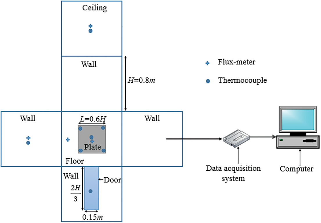
Figure 2: Experimental test local with flux-meters and thermocouples positions

2.2 Numerical Method

2.2.1 Test Local Modeling

The last configuration is projected on the vertical medium contained the glazed door (Fig. 3).

Figure 3: 2D simulated configuration at medium vertical projection

This is later simulated in two dimensions (2D) by considering a square cavity of side H. Filled with air, the system is heated from underneath by a heat source characterized by a width of L=60%H and a consistent temperature of Th. The ceiling, along with the remaining floor (excluding the iron plate) and all vertical walls, are treated as adiabatic surfaces. However, a section of one vertical wall is designated to replicate a glass door at a lower temperature, Tc.

2.2.2 Lattice Boltzmann Method Formulation

The Lattice Boltzmann Method (LBM) is a numerical method utilizes two single particle distribution functions, fk(r,t) for dynamic field and gk(r,t) thermal field. Considering the model D2Q9: two-dimensional (2D) and nine discrete velocities, Fig. 4. The viscous heat dissipation effect can be ignored for incompressible flow applications, allowing for the utilization of a basic Lattice Boltzmann Method (LBM) [35].

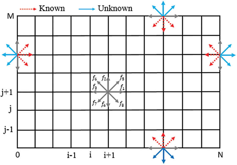
Figure 4: Lattice model D2Q9 with known an unknown distribution functions

The Lattice Boltzmann Equation (LBE) without external forces associated to the BGK (Bhatangar-Gross-Krook) approximation as for single particle and single time relaxation can be written [32,35,36]:

∂fk(r,t)∂t+ck∂fk(r,t)∂x=−1τm(fk(r,t)−fkeq(r,t))(1)

The equilibrium distribution function can be expressed as in [37]:

fkeq(r,t)=ωkρ(r,t)(1+3ck→.u→c2+92(ck→.u→)2c4−32u→.u→c2)(2)

The weights factors ωk and the discrete velocity coordinates ckx=Δx/Δt, cky=Δy/Δt for D2Q9 are given as follows:

ω0=49 (stationary particle), ω1−4=19, ω5−8=136

c→0=(0,0), c→1−4= (±1,0);(0,±1), c→5−8=(±1,±1)

Notice that, Δx, Δy and Δt are the lattice for space and time step, respectively, which are fixed to unity (Δx=Δy=Δt=1).

For dynamic field the LBE-BGK with external buoyancy forces can be written as:

fk(r+ckΔt,t+Δt)=(3ν−0.53ν+0.5)fk(r,t)+13ν+0.5fkeq(r,t)+Δt3ωkρgβΔT.ckyc2(3)

For thermal field the LBE-BGK can be written as:

gk(r+ckΔt,t+Δt)=(3α−0.53α+0.5)gk(r,t)+13α+0.5gkeq(r,t)(4)

The equilibrium distribution function for thermal field can be developed at first-order [38,39].

gkeq(r,t)=ωkT(r,t)[1+3ck→.u→c2](5)

Finally, the basic quantities, such as density ρ(r,t), velocity vector u→(r,t) and temperature T(r,t) are obtained by using the summations:

ρ(r,t)=∑08fk(r,t)(6)

ρu→(r,t)=∑08ck→fk(r,t)(7)

T(r,t)=∑08gk(r,t)(8)

2.2.3 Boundary Conditions

The boundary conditions relevant to the problem within a two-dimensional (2D) framework.

•   Dynamic boundary conditions:

✓   On the walls all velocities are zero: u=v=0

✓   « bounce-back »

fk(r,t)=fopp(k)(r,t)(9)

•   Thermal boundary conditions:

The equation provided was utilized to determine the prescribed temperature applied to both the hot and cold walls. θ=T−TcTh−Tc is the dimensionless form of temperature.

gk(r,t)=(ωk+ωopp(k))θ−gopp(k)(r,t)(10)

✓   On the square plate (heat source:y=0 and (H−L)2≤x≤(H+L)2) the imposed temperature Th≈35°C, which give θh≈1.

✓   On the door (cold portion:x=H and 0≤y≤3H2) the imposed temperature Tc≈18°C, which give θc≈0.

✓   On the adiabatic walls ceiling and the rest of the floor (without the iron plate) and all the vertical walls (without the door): ∂T∂n=∂θ∂n=0, where n is the normal of walls (x or y).

For example, at the ceiling (top wall (y=H→M) and (0≤x=i≤H→N)), we employed this numerical approximation for calculations.

gk(i,M)=gk(i,M−1)(11)

Here, “i” corresponds to the iteration index along the x-direction, and “M” signifies the count of lattice points located at the upper wall, as illustrated in Fig. 4.

3  Results and Discussion

The results will be qualitatively presented in terms of the temperature profiles T(°C) and the heat flux densities φ(W/m2) in various positions/faces in the test local. Moreover, the time evolution of the temperature at the center of the cavity and the temperature profiles along the vertical centerline will be compared with those obtained numerically by lattice Boltzmann method for the plate of width L=0.6 H and the imposed temperature in the plate Th≈35°C and in the door Tc≈18°C.

The objective here is to link between the experimental model and the numerical model, and transform lattice units into physical units just to compare the results. For the first time, we calculate Rayleigh number Ra=gβΔTH3/(αν), using proprieties of air and the parameter of physical problem H=0.8 m and ΔT=Th−Tc.

The numerical code (LBM–FORTAN) is used in two dimension (2D) by considering the projection of the experimental configuration on the vertical medium contained the glazed door (Fig. 3). The lattice dimensions are set as N = 800 for the x direction and M = 800 for the y direction. The lattice spacing intervals, Δx and Δy, as well as the lattice time step, Δt, are all assigned a value equal to unity.

Utilizing the principle of similarity and dimensionless parameters like the Rayleigh number (Ra) and Prandtl number (Pr) for the air-filled cavity, we are able to compute the value of gβ as depicted in Eq. (3) gβ=Raαν/(ΔTH3). In lattice units, the option exists to select ν = 0.02 (or any alternative value, provided it remains modest, below 0.1). From the time when Pr=ν/α=0.71; then α=0.02/0.71; supposing that ΔT→Δθ=1 and H=M.Δy; here, with a lattice spacing of Δy=1 and M representing the quantity of nodes in the y direction, we arrive at the point where we can perform calculations. gβ=Ra(αν)/(M3).

The results obtained from the lattice Boltzmann method are expressed in lattice units. For the temperature, we used θ=(T−Tc)/(Th−Tc) to convert these values at the physical units.

3.1 Calibration and Tests of the Experimental Model

Before starting our monitoring, it is recommended that the validity of the measurements be guaranteed. For that, we realized two tests: the first one is made without a heat source. We ensured that all the thermocouples and the flux-meters indicate the same values. The second test is realized with the presence of the heat source. The iron plate is heated for 12 h and goes off for 12 h. The measurements are presented in terms of time evolution of temperature and the heat flux densities through the envelope of cavity for a plate of width L and for an adjustable set point heat source Th. These results guarantee that all thermocouples and flux-meters are operational and also show that the duration of 6 h is sufficient to reach steady state. For the following measures, the heat source is switched on for 6 h and goes off in 6 h as a cycle.

3.2 Thermal Profiles

Fig. 5 shows the variation of imposed temperature of the plate in which the set point temperature is kept constant at Th≈35°C. The same figure presents the variation of outdoor air temperature which is controlled by an air conditioner Tc≈18°C for two cycles. When the heat source is switched on, the temperature increases to the set point with a delay of 6 h, then decreases towards a minimum temperature around Tc when the heat source is switched off in the same delay. It should be noted that the heating of the plate is provided by a lamp of 100W placed just down the center of it (Fig. 1). The delay marked by the curve relative to the hot plate is related to the average temperature measured by five thermocouples placed in the center and in the angles of the square plate.

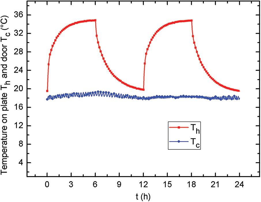
Figure 5: Time evolution of imposed temperatures Th and outdoor temperature Tc

The time evolution of the measured temperature of the plate, door, ceiling, center and wall are shown in Fig. 6 for two heating cycles. These curves show that during the heating period, the temperature curves behave in the same way. These increase to a maximum when the heat source is switched on and then decrease to a minimum when the heat source is turned off. We also find that the coldest wall is at the glass door. Its maximum temperature remains not higher than 22.50°C and remains close to that of the outside (≈18°C). Note that the curves relating to the temperatures in the center and on the inner face of the ceiling of the cavity are almost confused. This justifies the thermal insulation of the walls, especially the ceiling. In this case, the flux transmitted by the convection of ambient air to the ceiling, then through the ceiling to the outside, is almost negligible. This is shown by the measurements of the heat flux densities (Fig. 7). On the other hand, the maximum of temperature on the ceiling is much higher than that of the other walls (≈24.30°C). Its relative curve is close to that of the temperature at the center of the test local, its maximum (≈27°C). This is visualized by the thermal structure (isotherms) in two dimensions in Fig. 8, in the upper half, the temperature is almost identical.

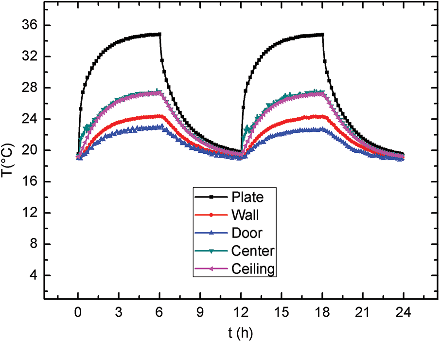
Figure 6: Time evolution of temperatures at different positions

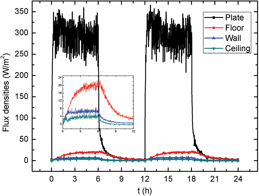
Figure 7: Time evolution of heat flux densities at different faces

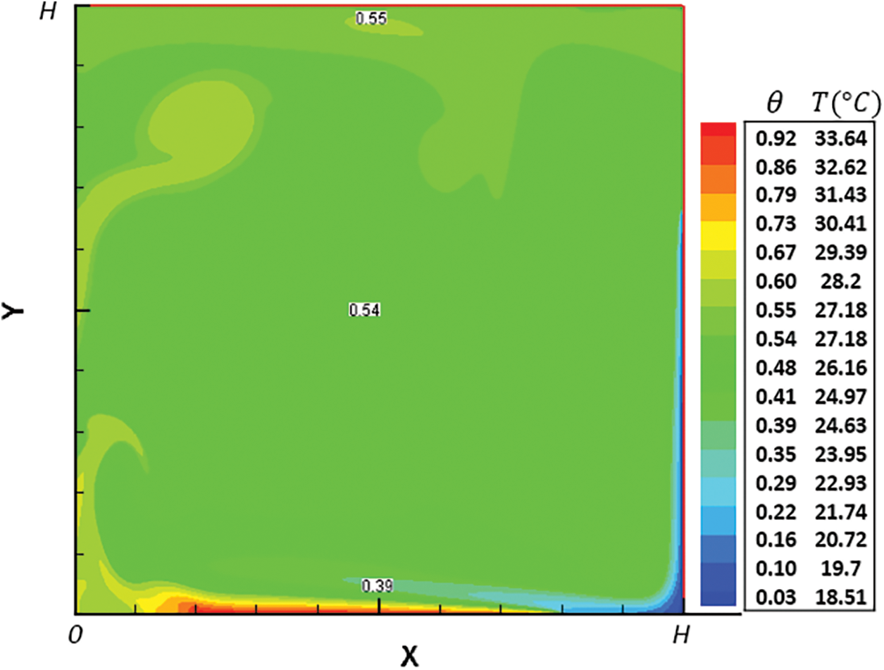
Figure 8: Thermal field structure in 2D

3.3 Heat Flux Densities

We specify here that at the level of the floor, there is an iron plate placed in the center of the floor (Fig. 1). For these, we have access to two densities of flow: the first through the wooden part and the other through the hot metal plate. This last flux density will not be studied in time because its average value is negligible. However, the heat flux density at the center of the plate will be considered.

The heat flux densities measured in the center of the surface of the plate, the floor, the wall and the ceiling are shown in Fig. 7. Firstly, there is no recorded delay between the curves of flux, which explains the low thermal inertia of the walls. Note also that the heat flux density through the ceiling and the walls is very low compared to the plate. Negative values of this flux density that appear during the stopping phase of heating show that there is a slight return of heat stored in the ceiling towards the cavity. When the heat source is switched on, the curves of these heat flux densities increase from an initial value of almost zero to a maximum φmax, with rapid oscillations around an average value. Note that at t=6 h, the heat flux density of the plate oscillates rapidly around an average value equal to 300W/m2, the floor 20W/m2, the wall 6W/m2 and the ceiling 4W/m2. While the values of the heat flux density of the walls and the ceiling remain practically negligible compared to the heat flux density of the plate, this indicates that there is thermal insulation in the walls and the ceiling. This justifies roughly the consideration of the adiabatic walls in the simulation part. When the heat source is turned off, the relative heat flux density of the ceiling drops rapidly to zero, while those of the vertical walls and the floor gradually decrease to a minimum value near zero. Indeed, even if we stop the heating lamp, the floor remains relatively hot due to hot air trapped in a false floor below (a false floor in which the lamp is fitted). We can see that even at the end of the shutdown phase (t=12 h), the heat flux density crossing the floor is 3W/m2. From the flu-meters we can measure the heat flux densities on different faces, considering the number of existing the flux-meters. By the thermocouples, we measured the temperatures in different positions, inside or outside. By considering the steady state and the propriety of the envelope, we can calculate all the heat fluxes in order to check in the next part.

3.4 Analysis of the Temperature and Heat Flux

According to the analysis of the temperature and flux density measurements, we arrive at several verifications. The numerical study in the part below is based on these checks, especially in the permanent regime. One of the remarks that must be emphasized is that from one cycle to another. For each position, the temperature and the heat flux density return to their initial value (that of the start for the first time). This means that the cavity, including its envelope, is completely discharged and there is almost no heat storage effect going from one cycle to another. These are the problems related to the low thermal inertia of the envelope. At the permanent regime, t=6 h for the first cycle or t=18 h for the second cycle, we can determine the maximum of the measured parameters considering the average value. Table 1 shows the maximum values of the temperature measured in each position for the outer and inner faces. These values show that the temperature of the door is the lowest compared to those of the wall and ceiling. However, the maximum values of the heat flux densities measured in each face are shown in Table 2. We can determine at the permanent regime the maximum of the measured flux by the relation ϕ=φ.S, and the maximum of the calculated flux by the relation ΔT=Rth.ϕ. Where S(m2), e(m), λ, Rth(K/W)=∑eλS and ΔT=Tmax−Tc are the surface of the face, the thickness of the layer, the thermal conductivity, thermal resistance and the difference of the temperature between the maximum temperature in the inner face and outside face, respectively. The considered proprieties (e, λ) of each layer are given by: plywood (e=0.3 cm, λ=0.15 W/(mK)), polystyrene (e=3 cm, λ=0.03 W/(mK)) and for the glass (e=0.4 cm, λ=1W/(mK)).

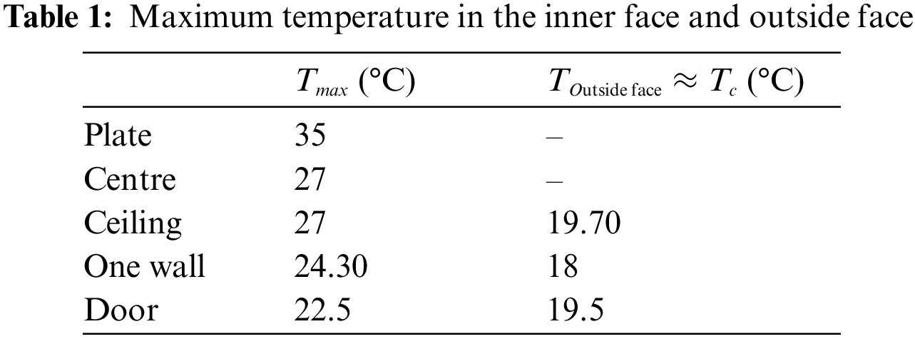
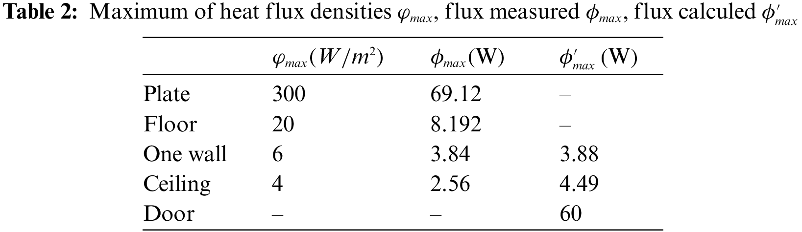
The temperature of the interior and exterior faces was measured to calculate the heat flux. This latter is measured directly considering the heat flux densities measured in some faces. But in certain faces, it is calculated by the following expression ϕ=(Tmax−TOutside face)/Rth in the permanent regime. The flow produced by the plates is the greatest. On the other hand, the flow left by the ceiling and each wall is very weak, which guarantees the insulation of the envelope of the studied local. Notice that a large part of the flow entered from the plate and from the floor is lost through the door.

3.5 Comparison between Experimental and Numerical Results

The comparison between the experimental and numerical results is presented in terms of temporal variation of the temperatures at the center of the cavity and along the vertical median axis for L=0.6 H; Th≈35°C and Tc≈18°C. The choice of these two temperature profiles (center and vertical median) comes from the intersection of the vertical projection planes. The center and the vertical median are identical for 2D and 3D. Generally, heat transfer is studied experimentally and numerically by several authors in 2D and 3D configurations [40,41]. The 3D cavities can be reduced to 2D based on a few criteria, such as symmetry and aspect ratio etc., without forgetting the constraints of calculation by simulation and the performance of the machines used. In the present problem, the vertical mid-plane, which comprises the door and the plate, is considered as a plane of symmetry. Moreover, the center and the vertical axis passing through the center are common points between the 3D and 2D configurations. This is the second reason why the comparison is made precisely for the evolution of the temperature at the center for a heating cycle and for the temperature profile along this axis at t = 6 h. Note that, the LB model is dimensionless. So, the results found by simulation are also in dimensionless form (to avoid numerical problems and stability). From the expression of the dimensionless temperature θ=(T−Tc)/(Th−Tc) and the obtained results by simulation, we can determine the temperature values with dimension (°C) using the following transformation T=θ(Th−Tc)+Tc. This transformation is used to fit the numerical results with the experimental results. Starting by a simulation of the temperature distribution in 2D by consideration of the vertical mid-plane, which includes the door and the plate. The temperature field structure at t=6 h is presented in Fig. 8, with dimensionless temperature values, indicated in the legend with different colors. This is just to justify and guarantee the comparison concerning the experimental and the numerical results. Note that, in the upper half the temperature values are identical, which justifies the coincidence of the temperature curves in the center and in the ceiling presented in Fig. 6. Other comparisons were carried out to consolidate this study. Fig. 9 shows the time evolution of the temperature at the center of the test local during a heating cycle (6 h). The comparison of the two curves indicates that there is a good agreement between the curves of variations of the two temperatures obtained experimentally and numerically. The temperature profile along the vertical centerline of the cavity T(H/2,Y) is presented in Fig. 10 at t=6 h. The temperature decreases to a minimum in the region 0≤Y≤10 cm and increases to a fixed value close to 27°C, which shows that when Y≥20 cm, there is a thermal stratification. The temperature lowest point within this region indicates a substantial influx of cold air, propelling the warm air to maintain its rotational motion along with the displacement of a certain volume of hot air by the colder counterpart (Fig. 8). A comparison of the experimental and numerical findings demonstrates a close alignment in temperature, with a difference does not exceed of ±1°C. According to the conditions of the experiment and the measurement errors by the thermocouples (±1°C), as well as the assumptions of the simulation. It is normal to find an acceptable deviation between the experimental results and the numerical results.

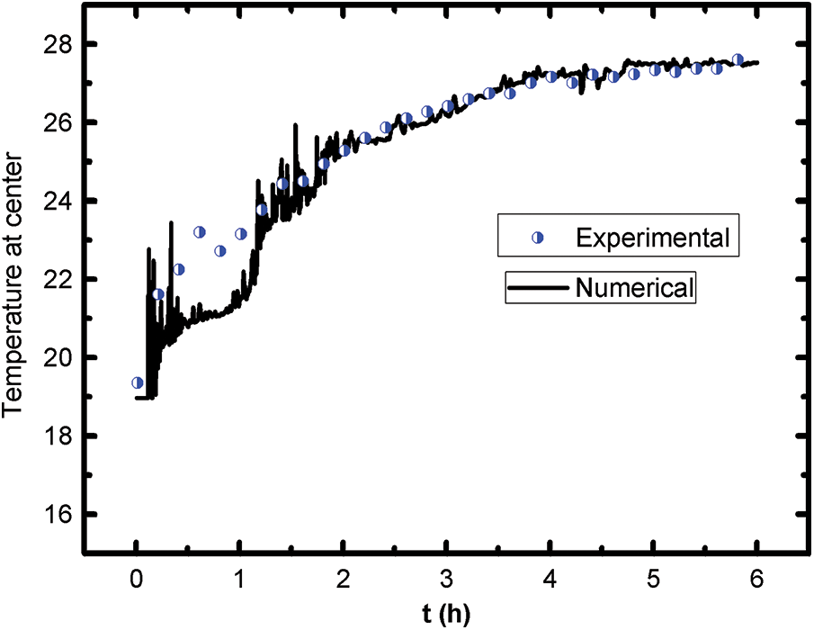
Figure 9: Time evolution of temperature at center of cavity

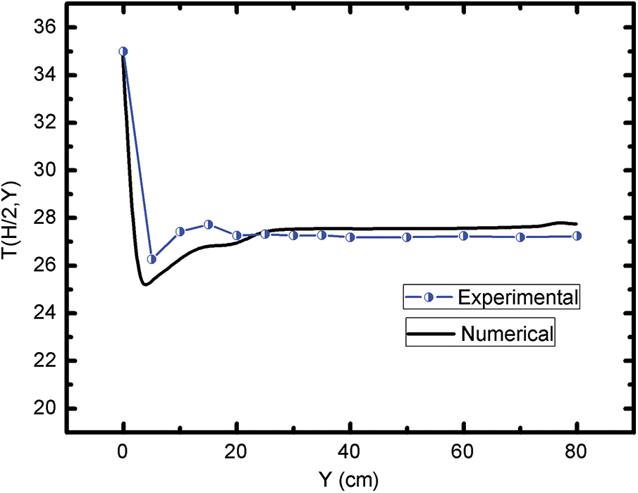
Figure 10: Temperature profile along the vertical center ligne Y of cavity

4  Conclusion

In the present paper, we executed both an experimental and numerical analysis of convective heat transfer within a cubic test model. The description of the studied cavity, as well as the construction materials and measuring equipment, was detailed at the beginning of the paper. We also tested the validity of temperature and heat flux measurements by performing tests to calibrate thermocouples and flux meters. In the second step, we conducted a numerical study in two dimensions (2D) based on the lattice Boltzmann method in order to make a comparison between the experimental and numerical results. The results are shown in terms of temperatures as a function of time and heat flux densities across the envelope during two heating/cooling cycles. An examination of the thermal field and the heat flux densities allowed us to conclude that:

-In heating cycles, temperature and heat flux densities on different positions/faces increase with time, but in cooling cycles, temperature and heat flux densities are decreased.

-In the test local, the cold part is the door, and the hot part is at the plate.

-The heat flux measured ϕmax and calculaled ϕmax′ is compared with a considered difference in each face.

-A large part of the flow entered from the plate is lost through the door.

-In the upper half of the test local, the temperature values are almost identical. The temperature curves in the center and in the inner face of the ceiling are practically confused. This coincidence is also justified by the temperature field presented by the lines isotherms.

-The evolution of the temperature at the center and the temperature profile along the vertical axis passing through the center found by the numerical study and the experimental study were compared and interpreted during one heating cycle. The results obtained show good agreement with a difference that does not exceed ±1°C.

Finally, this computational investigation was undertaken with the aim of creating and confirming a proprietary code utilizing the lattice Boltzmann method (LBM). This code facilitates the treatment of heat transfer within building simulations, as well as the analysis of natural or mixed convection flows within intricate geometries. It caters to both laminar and turbulent regimes and accommodates both 2D and 3D configurations.

Acknowledgement: The authors would like to thank the National Center for Scientific and Technical Research (CNRST) for access to computing machines.

Funding Statement: The authors received no specific funding for this study.

Author Contributions: All authors contributed to the study conception and design. Material preparation, data collection and analysis were performed by Noureddine Abouricha, Ayoub Gounni and Mustapha El Alami. The first draft of the manuscript was written by Noureddine ABOURICHA and all authors commented on previous versions of the manuscript. All authors read and approved the final manuscript.

Availability of Data and Materials: There is no unavailable data in this study.

Conflicts of Interest: The authors have no competing interests to declare that are relevant to the content of this article.

References

1. Kuznik, F., David, D., Johannes, K., Roux, J. J. (2011). A review on phase change materials integrated in building walls. Renewable and Sustainable Energy Reviews, 15(1), 379–391. [Google Scholar]

2. Jin, X., Medina, M. A., Zhang, X. (2013). On the importance of the location of PCMs in building walls for enhanced thermal performance. Applied Energy, 106, 72–78. [Google Scholar]

3. Mohammed, M. A., Derea, A. T., Lafta, M. Y., Ali, O. M., Alomar, O. R. (2023). Effect of nanomaterials addition to phase change materials on heat transfer in solar panels under Iraqi atmospheric conditions. Frontiers in Heat and Mass Transfer, 21, 215–226. [Google Scholar]

4. Gendelis, S., Jakovičs, A., Ratnieks, J. (2017). Thermal comfort condition assessment in test buildings with different heating/cooling systems and wall envelopes. Energy Procedia, 132, 153–158. [Google Scholar]

5. Rashid, Y., Alnaimat, F., Mathew, B. (2018). Energy performance assessment of waste materials for buildings in extreme cold and hot conditions. Energies, 11(11), 3131. [Google Scholar]

6. Shaikh, U. I., Sur, A., Roy, A. (2023). Performance analysis of an energy efficient pcm-based room cooling system. Frontiers in Heat and Mass Transfer, 20, 1–10. https://doi.org/10.5098/hmt.20.28 [Google Scholar] [CrossRef]

7. Sonnick, S., Erlbeck, L., Schlachter, K., Strischakov, J., Mai, T. et al. (2018). Temperature stabilization using salt hydrate storage system to achieve thermal comfort in prefabricated wooden houses. Energy and Buildings, 164, 48–60. [Google Scholar]

8. Wang, X., Li, W., Luo, Z., Wang, K., Shah, S. P. (2022). A critical review on phase change materials (PCM) for sustainable and energy efficient building: Design, characteristic, performance and application. Energy and Buildings, 260, 111923. [Google Scholar]

9. Østergaard, D. S., Svendsen, S. (2016). Case study of low-temperature heating in an existing single-family house—A test of methods for simulation of heating system temperatures. Energy and Buildings, 126, 535–544. [Google Scholar]

10. Khoukhi, M. (2018). The combined effect of heat and moisture transfer dependent thermal conductivity of polystyrene insulation material: Impact on building energy performance. Energy and Buildings, 169, 228–235. [Google Scholar]

11. Kürekci, N., Özcan, O. (2012). An experimental and numerical study of laminar natural convection in a differentially-heated cubical enclosure. ISI Bilimi VE Teknigi Dergisi-Journal of Thermal Science and Technology, 32, 1–8. [Google Scholar]

12. Piña-Ortiz, A., Hinojosa, J. F., Navarro, J. M. A., Xamán, J. (2018). Experimental and numerical study of turbulent mixed convection in a cavity with an internal heat source. Journal of Building Physics, 42(2), 142–172. [Google Scholar]

13. Troppová, E., Tippner, J., Švehlík, M. (2018). Numerical and experimental study of conjugate heat transfer in a horizontal air cavity. Building Simulation, 11(2), 339–346. https://doi.org/10.1007/s12273-017-0403-y [Google Scholar] [CrossRef]

14. Zheng, Q., Wang, H., Ke, Y. (2023). Prediction of the local and total thermal insulations of a bedding system based on the 3D virtual simulation technology. In: Building simulation, vol. 16, no. 8, pp. 1467–1480. Beijing, China: Tsinghua University Press. [Google Scholar]

15. Wei, Y., Dou, H. S., Wang, Z., Qian, Y., Yan, W. (2016). Simulations of natural convection heat transfer in an enclosure at different Rayleigh number using lattice Boltzmann method. Computers & Fluids, 124, 30–38. [Google Scholar]

16. Crouse, B., Krafczyk, M., Kühner, S., Rank, E., van Treeck, C. (2002). Indoor air flow analysis based on lattice Boltzmann methods. Energy and Buildings, 34(9), 941–949. [Google Scholar]

17. Abouricha, N., Ennawaoui, C., Alami, M. E. (2023). Amplitude and period effect on heat transfer in an enclosure with sinusoidal heating from below using lattice Boltzmann method. Frontiers in Heat and Mass Transfer, 21(1), 523–537. https://doi.org/10.32604/fhmt.2023.045914 [Google Scholar] [CrossRef]

18. Freile, R., Tano, M. E., Ragusa, J. C. (2024). CFD assessment of RANS turbulence modeling for solidification in internal flows against experiments and higher fidelity LBM-LES phase change model. Annals of Nuclear Energy, 197, 110275. [Google Scholar]

19. Abbasi, A., Safavinejad, A., Lakhi, M. (2023). Numerical study of surface radiation-natural convection entropy generation in a 2D cavity using the LBM. International Communications in Heat and Mass Transfer, 149, 107141. [Google Scholar]

20. Hu, M., Zhang, Z., Liu, M. (2023). Transient particle transport prediction based on lattice Boltzmann method-based large eddy simulation and Markov chain model. In: Building simulation, pp. 1–14. Beijing, China: Tsinghua University Press. [Google Scholar]

21. Borquist, E., Thapa, S., Weiss, L. (2016). Experimental and lattice Boltzmann simulated operation of a copper micro-channel heat exchanger. Energy Conversion and Management, 117, 171–184. [Google Scholar]

22. Zhou, B., Wu, X., Chen, L., Fan, J. Q., Zhu, L. (2021). Modeling the performance of air filters for cleanrooms using lattice Boltzmann method. In: Building simulation, vol. 14, pp. 317–324. Beijing, China: Tsinghua University Press. https://doi.org/10.1007/s12273-020-0660-z [Google Scholar] [CrossRef]

23. He, Y. L., Liu, Q., Li, Q., Tao, W. Q. (2019). Lattice Boltzmann methods for single-phase and solid-liquid phase-change heat transfer in porous media: A review. International Journal of Heat and Mass Transfer, 129, 160–197. [Google Scholar]

24. Nee, A. (2020). Hybrid lattice Boltzmann––Finite difference formulation for combined heat transfer problems by 3D natural convection and surface thermal radiation. International Journal of Mechanical Sciences, 173, 105447. [Google Scholar]

25. Liu, Z., Mu, Z., Wu, H. (2019). A new curved boundary treatment for LBM modeling of thermal gaseous microflow in the slip regime. Microfluidics and Nanofluidics, 23, 1–12. [Google Scholar]

26. Tao, S., Xu, A., He, Q., Chen, B., Qin, F. G. (2020). A curved lattice Boltzmann boundary scheme for thermal convective flows with Neumann boundary condition. International Journal of Heat and Mass Transfer, 150, 119345. [Google Scholar]

27. Tao, S., Chen, B., Xiao, H., Huang, S. (2019). Lattice Boltzmann simulation of thermal flows with complex geometry using a single-node curved boundary condition. International Journal of Thermal Sciences, 146, 106112. [Google Scholar]

28. D'Orazio, A., Karimipour, A. (2019). A useful case study to develop lattice Boltzmann method performance: Gravity effects on slip velocity and temperature profiles of an air flow inside a microchannel under a constant heat flux boundary condition. International Journal of Heat and Mass Transfer, 136, 1017–1029. [Google Scholar]

29. Zhao, Z., Wen, M., Li, W. (2021). A coupled gas-kinetic BGK scheme for the finite volume lattice Boltzmann method for nearly incompressible thermal flows. International Journal of Heat and Mass Transfer, 164, 120584. [Google Scholar]

30. Huang, Y., Xu, X., Zhang, S., Wu, C., Liu, C. et al. (2023). Thermodynamic characteristics of gas-liquid phase change investigated by lattice Boltzmann method. Applied Thermal Engineering, 227, 120367. [Google Scholar]

31. Lin, Y., Yang, C., Zhang, W., Fukumoto, K., Saito, Y. et al. (2023). Estimation of effective thermal conductivity in open-cell foam with hierarchical pore structure using lattice Boltzmann method. Applied Thermal Engineering, 218, 119314. [Google Scholar]

32. Wang, Z., Xie, K., Zhang, Y., Hou, X., Zhao, W. et al. (2023). A multiphase model developed for mesoscopic heat and mass transfer in thawing frozen soil based on lattice Boltzmann method. Applied Thermal Engineering, 229, 120580. [Google Scholar]

33. Abouricha, N., El Alami, M., Souhar, K. (2020). Lattice Boltzmann modeling of convective flows in a large-scale cavity heated from below by two imposed temperature profiles. International Journal of Numerical Methods for Heat & Fluid Flow, 30(5), 2759–2779. [Google Scholar]

34. Abouricha, N., El Alami, M., Gounni, A. (2019). Lattice Boltzmann modeling of natural convection in a large-scale cavity heated from below by a centered source. Journal of Heat Transfer, 141(6), 62501. [Google Scholar]

35. Kao, P. H., Yang, R. J. (2007). Simulating oscillatory flows in Rayleigh-Benard convection using the lattice Boltzmann method. International Journal of Heat and Mass Transfer, 50(17–18), 3315–3328. [Google Scholar]

36. Succi, S. (2001). The lattice Boltzmann equation: for fluid dynamics and beyond. UK: Oxford University Press. [Google Scholar]

37. He, X., Chen, S., Doolen, G. D. (1998). A novel thermal model for the lattice Boltzmann method in incompressible limit. Journal of Computational Physics, 146(1), 282–300. [Google Scholar]

38. Kefayati, G. R. (2013). Lattice Boltzmann simulation of MHD natural convection in a nanofluid-filled cavity with sinusoidal temperature distribution. Powder Technology, 243, 171–183. [Google Scholar]

39. Gaedtke, M., Wachter, S., Kunkel, S., Sonnick, S., Rädle, M. et al. (2020). Numerical study on the application of vacuum insulation panels and a latent heat storage for refrigerated vehicles with a large eddy lattice Boltzmann method. Heat and Mass Transfer, 56, 1189–1201. [Google Scholar]

40. Mellah, S., Cheikh, N. B., Beya, B. B., Lili, T. (2011). Comparaison 2D/3D du transfert de chaleur au sein d’une enceinte carrée/cubique remplie d’air. CFM 2011-20ème Congrès Français de Mécanique, Besançon, France. [Google Scholar]

41. Ampofo, F., Karayiannis, T. G. (2003). Experimental benchmark data for turbulent natural convection in an air filled square cavity. International Journal of Heat and Mass Transfer, 46(19), 3551–3572. [Google Scholar]