Diagnostic Method for Load Deviation in Ultra-Supercritical Units Based on MLNaNBDOS

Abbreviations

1  Introduction

With the rising share of renewable energy, traditional coal-fired power units are gradually shifting from being “primary energy suppliers” to “providers of flexibility resources” [1]. Enhancing the operational flexibility of these units has emerged as a paramount technical imperative within the coal-fired power generation sector. Advanced ultra-supercritical coal-fired power generation technology, operating at 650°C and above, delivers elevated efficiency in power generation and reduced emissions of pollutants and carbon. This technology is recognized as a crucial direction for efficient and clean utilization of coal [2].

Ultra-Supercritical (USC) units follow the load instructions from the grid dispatch center externally while maintaining energy balance and parameter stability within the boiler and turbine systems. However, issues such as steam-water mixing and inherent faults in primary and auxiliary equipment hinder the dynamic response of the coordinated control system (CCS) [3], resulting in deviations between the USC unit’s load output and the automatic generation control (AGC) load instructions. Such deviations affect the safe and stable operation of the unit and the grid load dispatch. Therefore, resolving the load deviation issues of USC units and identifying their causes is crucial for ensuring the unit’s safe and stable operation.

Currently, the methods for modeling load deviations in thermal power units can be broadly categorized into two types [4]: first-principles-based modeling methods and data-driven modeling methods.

First-principles-based modeling methods are founded on specific assumptions and utilize simplified physical model structures, employing the laws of mass conservation and energy conservation to analyze the operation processes of the system under study. For instance, Fan et al. [5] developed a dynamic nonlinear mathematical model for the wide-load-range operation of a USC once-through boiler-turbine unit. Xie et al. [6] introduced an improved separator steam dryness calculation method to avoid the issue of model switching between the reheating cycle model and the once-through model. However, due to the complexity of USC units, first-principles-based modeling methods often encounter difficulties in accurately depicting the operation process of the units based on limited knowledge. As a result, these models typically do not achieve high modeling accuracy [7].

In contrast to first-principles-based methods, data-driven modeling methods extract hidden, previously unrecognized, and potentially valuable information from extensive datasets, uncovering latent operational patterns of the units and providing decision support for real-time operation. Zhou et al. [7] constructed a regression model of thermal power unit operation data based on feature selection and optimized the unit operation using coal consumption as an indicator. Huang et al. [8] proposed a new data-driven modeling approach based on an improved transformer neural network and optimization algorithms for the boiler-turbine coupling process in CCS of ultra-supercritical units. Chen et al. [9] used a dual-driven mechanism and data modeling approach to model the unit and optimize the steam pressure and cold end system. Tang et al. [10] developed a multi-label random forest load deficiency diagnosis model based on an improved whale optimization algorithm, where the compound causes of load deficiency in thermal power units are constructed as binary multi-label relationships, thus identifying the equipment sources of load deficiency. Currently, data-driven modeling of thermal power units is mostly used to optimize unit operation based on certain aspects of operating parameters, and less research has been conducted on unit load-out diagnosis.

In addition, the issue of class imbalance in the operational data of thermal power units negatively impacts the classification performance of the model. Owing to the limited number of fault samples in the operational data of thermal power units and the insufficient types of existing fault samples to cover all possible faults, classification models may exhibit high accuracy for majority classes but perform poorly for minority classes. Therefore, addressing the class imbalance problem in thermal power unit datasets, reducing the impact of imbalanced data on the performance of classification models, and improving the accuracy of fault sample classification is of critical importance.

The utilization of resampling techniques to preprocess imbalanced datasets represents an effective approach to addressing the uneven distribution of samples in imbalanced datasets. Currently, resampling methods are relatively limited in the condition monitoring and diagnosis of USC thermal power units, with most efforts focused on fault diagnosis of power transformers and bearings, and limited applications in waste incineration power plants and AGC attack detection. Li et al. [11] introduced an adaptive clustering weighted oversampling method that assigns different oversampling weights and variable k-nearest neighbors to different samples, thereby increasing the representation of minority class samples. Hou et al. [12] developed a suitability model for waste incineration power plants based on the synthetic minority oversampling technique (SMOTE) combined with support vector machines, which reduces the impact of imbalanced data samples on model classification performance. Roy et al. [13] introduced a learning algorithm based on support vector data description that utilizes SMOTE to detect various false information in AGC systems.

Moreover, the natural neighbor theory [14] has been applied to the field of data oversampling, resulting in the development of various new methods, including NaNSMOTE [15], SMOTE-NaN-DE [16], NanBDOS [17], and NLDAO [18]. However, these methodologies primarily extend or enhance SMOTE in binary classification problems and do not adequately address the issue of class imbalance in multi-dimensional label problems. The adaptability of natural neighbors to multi-dimensional label datasets remains insufficiently explored and utilized.

In summary, this paper addresses the class imbalance problem present in the USC unit load deviation dataset by proposing a multi-label natural neighbor boundary oversampling technique (MLNaNBDOS) for the diagnosis of USC thermal power unit load deviations. Using the MLNaNBDOS method, this study precisely controls over the generation of new instances, effectively preventing the creation of noisy samples. This approach not only improves the class imbalance issue in the USC unit load deviation dataset but also optimizes and enhances the performance of load deviation diagnosis in USC units.

2  Problem Description

2.1 Explanation of the Causes of USC Unit Load Deviations

USC units have numerous equipment and a complex generation process. The USC unit consists of a boiler, turbine, generator, and various auxiliary equipment and systems. The production process of the USC unit is illustrated in Fig. 1. Initially, pulverized coal is introduced into the furnace under the impetus of primary air, where it combusts to heat the feedwater within the water wall. This process causes the heated feedwater to evaporate, creating high-pressure steam. This steam propels the turbine rotor, enabling it to rotate and perform mechanical work. Subsequently, the turbine is linked to the generator via a coupling, which then produces electricity. Following this, the steam in the low-pressure cylinder condenses into feedwater in the condenser. After preheating in the regenerative system, the feedwater is reintroduced into the furnace. Finally, the flue gas produced are processed through dust removal, desulfurization, and denitrification before being released into the external environment, thereby completing the production process of the USC unit [10]. The USC unit’s production process encompasses multiple stages and involves coordinated operation of multiple systems. This includes managing auxiliary equipment and systems, performing system cleanings during cold startup, igniting the boiler, and operating the unit’s AGC system and CCS.

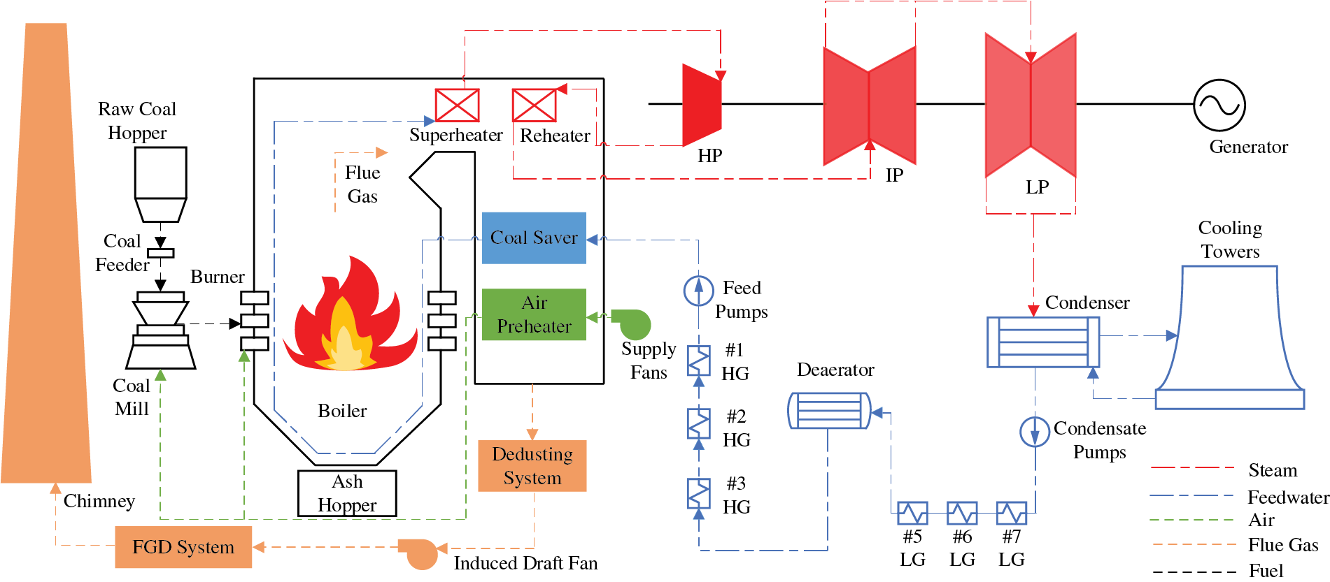
Figure 1: USC unit production process

The load output of a USC unit depends on two aspects. On one hand, it relies on the combined output of the three principal components: boiler, turbine, and generator. On the other hand, it depends on the load output of the supporting auxiliary equipment and systems. The unit’s actual load output can adequately meet the AGC load command requirements only when there is a precise alignment between the load output of auxiliary equipment and that of the main machines. Although the deviation between the AGC load command and the unit output can be detected and minimized by control theory, when a unit is underpowered, the equipment and systems associated with it are affected.

When load deviation occurs in USC units, a chain reaction can be triggered. For example, a decrease in the unit’s fuel consumption may implicate several components, such as coal mills and primary air fans. Similarly, an excessively high concentration of sulfur dioxide at the outlet of the desulfurization tower could indicate either an increased sulfur content in the coal or a reduced pressure in the slurry circulation pump. The resulting composition of multi-label load bias cause data samples degrade the classification performance of data-driven models.

2.2 Class Imbalance in USC Unit Load Deviation Data

The dataset of load deviation causes in USC units demonstrates a significant class imbalance issue. Typically, USC thermal power units generally operate under normal conditions. Load deviation data are generated exclusively when the units are in load-following mode or when faults occur. This results in a disproportionate distribution of data between load deviations and normal operation.

Given the high cost of obtaining load deviation data and the insufficiency of existing causes to cover all faults, some categories of load deviation causes exhibit class imbalance. This imbalance tends to increase the classification accuracy for the majority class labels while reducing the performance for minority class labels.

To address the class imbalance, this paper introduces the MLNaNBDOS method, which consists of three steps. First, it improves the traditional binary oversampling strategy by constructing the load deviation causes of thermal power units as binary multi-label relationships. The label power-set method [19] is introduced to preserve complex correlations between data. Second, based on the natural neighbor search strategy [14], the oversampling factor is adjusted to adaptively determine the oversampling factor and sampling weight for each class, thereby enhancing the balance of the imbalanced dataset. Finally, the method improves the generation of new instances by dynamically evaluating the similarity between the new instance and its natural neighbors, using a stochastic element to precisely control the process and prevent the generation of noisy samples.

3  Proposed Model

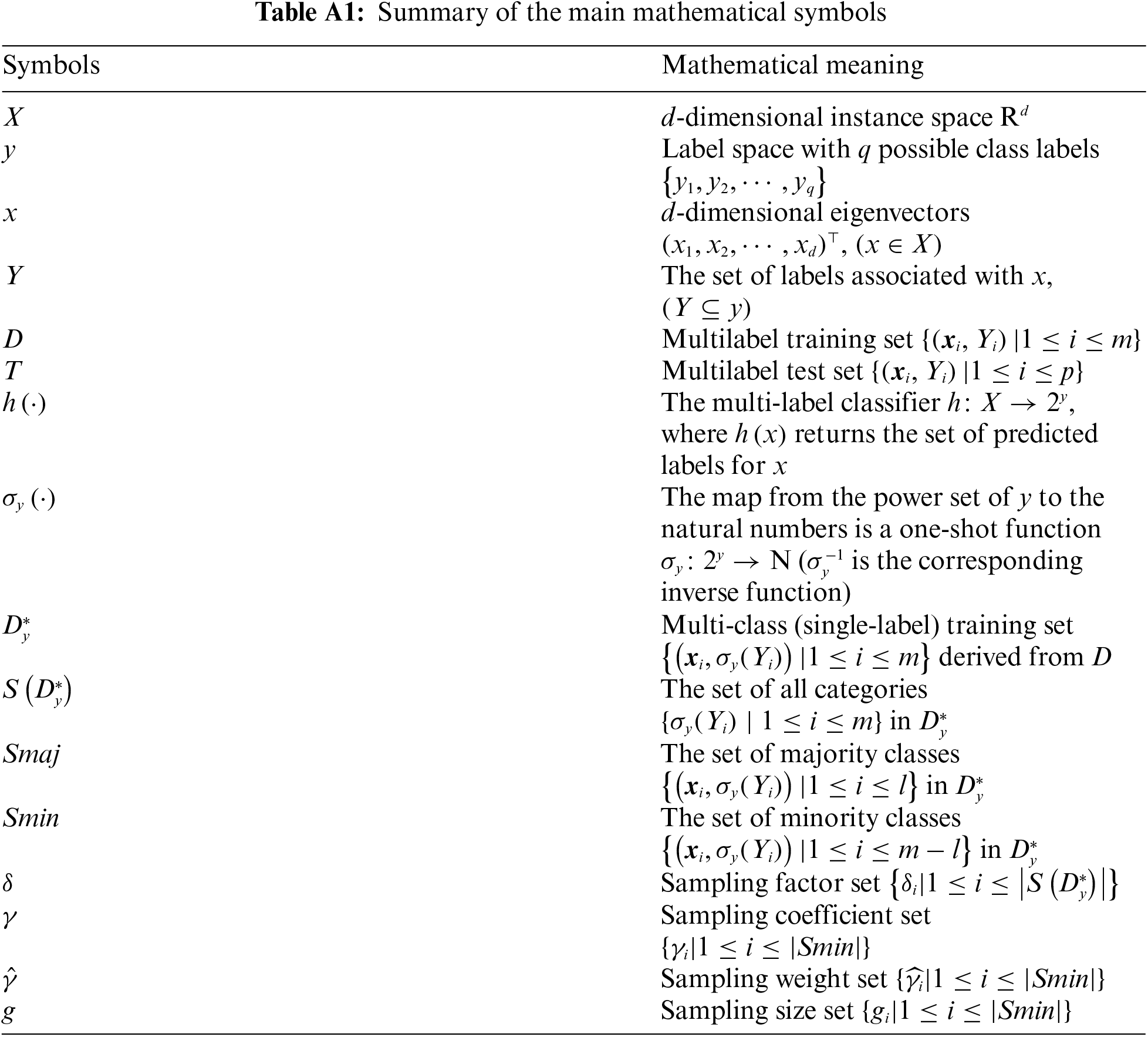
For ease of reference, Table A1 in Appendix A lists the main symbols used in the following text along with their mathematical meanings. The MLNaNBDOS method will be introduced through multi-label to multi-class conversion and natural neighbor search.

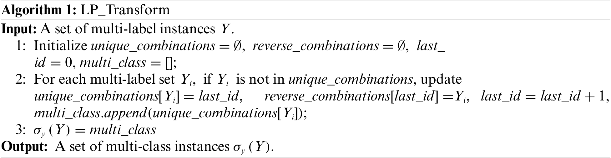
3.1 Multi-Label to Multi-Class Conversion

The label power-set (LP) method [19] is a direct approach to converting a multi-label learning problem into a multi-class (single-label) classification problem. Let σy:2y→N be an injective function that maps the power set of y to natural numbers, with σy−1 as its corresponding inverse function. During the training phase, the LP method first converts the original multi-label training set D into a multi-class (single-label) training set Dy∗. In this transformation, each distinct label set in D is considered as a new class.

Dy∗={(xi,σy(Yi))∣1≤i≤m}(1)

where, the set of all new classes in Dy∗ corresponds to S(Dy∗).

S(Dy∗)={σy(Yi)∣1≤i≤m}(2)

It is evident that |S(Dy∗)|≤min(m,2|y|) holds true. Subsequently, a classifier is trained on S(Dy∗). Ultimately, any multi-label training instance xi will be reassigned to the newly mapped single class σy(Yi). This instance then participates in the multi-class classifier training.

For a test instance xj, LP maps it back to the power set of y using σy−1 based on the prediction result of the multi-class classifier, thereby obtaining the corresponding label set Yj. Algorithm 1 outlines the detailed process of the LP transformation from multi-label to multi-class.

3.2 Natural Neighbor Search

Natural neighbors derived from the concept of neighborhood relationships observed in real-world social networks [14]. The idea is analogous to true friendships: when each individual in a society has at least one friend, a harmonious social relationship emerges [20]. This concept can be extended to the data domain, where it helps in forming a stable structure of natural neighbors. To clarify the discussion, the following definitions are provided.

Definition 1 (k-Nearest Neighbor): If xj∈X is a k-Nearest Neighbor (kNN) of xi∈X, then it satisfies the condition dist(xi,xj)≤dist(xi,xt). Here, xt is the kth nearest neighbor of xi, and dist(xi,xj) represents the Euclidean distance ‖xi−xj‖ between xi and xj.

The kNNs of xi can be determined as shown in Eq. (3).

kNNs(xi)={xj|dist(xi,xj)≤dist(xi,xt)}(3)

Once the value of k is set, kNNs(xi) can be efficiently computed using simple methods or a K-Dimensional tree (K-D tree) [17].

Definition 2 (Natural Neighbor): xj is considered a Natural Neighbor (NaN) of xi if and only if xj is a λ-Nearest Neighbor (λNN) of xi and xi is a λNN of xj. In other words, xj∈NaNs(xi)⇔xj∈λNNs(xi)∧xi∈λNNs(xj), where λ is referred to as the natural neighbor characteristic value.

In the kNN paradigm, the value of k is preset as a fixed number. However, natural neighborhood approach treats λ as an adaptive k-value that is suited to different datasets and is determined through natural neighbor search. The pseudocode for the search for natural neighbors (NaNs_Search) is provided in Algorithm 2. Following several iterations, a stable structure of natural neighbors in the instance space X is formed, as described in Eq. (4).

(∀xi)(∃xj)(r∈λ)∧(xi≠xj)→(xj∈rNNs(xi))∧(xi∈rNNs(xj))(4)

In Algorithm 2 (NaNs_Search), the number of iterations r increases from 1 to λ. The variable num counts the number of instances that are not considered as neighbors by any other instances. The algorithm stops once num no longer changes, indicating that the stable structure of natural neighbors has been formed. Additionally, Algorithm 2 incorporates the concept of Reverse k-Nearest Neighbors [21].

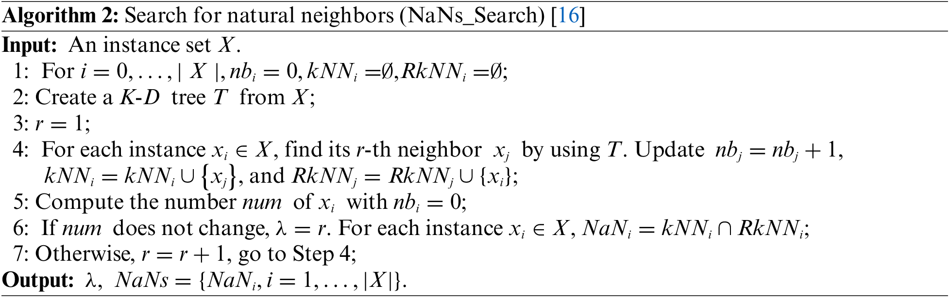
Definition 3 (Reverse k-Nearest Neighbor): If xj is a Reverse k-Nearest Neighbor (RkNN) of xi, this means that xi is one of the kNNs of xj.

The RkNNs of xi can be determined as shown in Eq. (5).

RkNNs(xi)={xj|xi∈kNNs(xj)}(5)

In summary, the NaNs of xi can be obtained through Eq. (6).

NaNs(xi)=kNNs(xi)∩RkNNs(xi)(6)

3.3 MLNaNBDOS

Based on the natural neighbor information obtained from Algorithm 2, noise and outliers in this study are defined as follows:

Definition 4 (Noise): If an instance xi satisfies ∀xj∈NaNs(xi), where σy(Yj)≠σy(Yi), then it is considered noise in set X.

According to Definition 4, if xi is a minority class instance, but all its natural neighbors belong to other classes, it will be treated as noise.

Definition 5 (Outlier): If an instance xi satisfies |NaNs(xi)|=0, then it is considered an outlier in set X. Here, |NaNs(xi)| denotes the cardinality of NaNs(xi).

According to Definition 5, if an instance xi has no natural neighbors, it will be classified as an outlier.

Based on Definitions 4 and 5, data preprocessing is performed on the original dataset to eliminate noise and outliers.

Boundary instances contain crucial classification information. During model training, boundary instances directly influence the model’s classification decisions. Therefore, during the process of oversampling minority class instances, this study selects minority class boundary instances as the base instances for oversampling. The definition of minority class boundary instances is delineated below:

Definition 6 (Minority Class Boundary Instance): For xi∈Smin, if xi is neither noise nor an outlier, and ∃xj∈NaNs(xi) such that σy(Yj)≠σy(Yi), then xi is considered a minority class boundary instance.

According to Definition 6, minority class boundary instances are required to have natural neighbors belonging to other classes. If a minority instance’s natural neighborhood consists entirely of instances from other classes, it is no longer considered a boundary instance. Instead, it is reclassified as noise (in accordance with Definition 5).

3.3.1 Intelligent Adjustment of the Oversampling Factor

Based on natural neighbor information, all minority class boundary instances in the training set are identified and stored in a Temporary Set (TS). It should be noted that if TSσy(Yi)=∅, meaning that no boundary instances are found for all minority class instances with class label σy(Yi), then these minority class instances are stored in TS. Next, the sampling factor δ for each class is calculated using Eq. (7), determining whether all or only some instances in each minority class within TS are subjected to oversampling.

δσy(Yi)=|Smaj|−|Sminσy(Yi)||TSσy(Yi)|(7)

If δσy(Yi)<1, partial oversampling of minority class instances in TS with class label σy(Yi) is performed to balance the dataset. Otherwise, all minority class instances in TS with class label σy(Yi) are selected. The instances selected as the basis for oversampling in TS are stored in the Base Instance Set (BIS), and the sampling coefficient γi for each base instance xi is calculated using Eq. (8).

γi=Δi|NaNs(xi)|(8)

where, Δi represents the number of minority class instances in NaNs(xi). The γ values are normalized using Eq. (9) to obtain the sampling weights γ^i for each base instance xi.

γ^i=γi∑γi(9)

A random selection of gi instances from NaNs(xi) is linearly interpolated with xi.

gi=round(γ^i×(|Smaj|−|Sminσy(Yi)|))(10)

where, round(⋅) denotes the rounding operation.

Assuming xt is selected, the generation process for the new instance xnew is as follows:

xnew=xi+random(0,1)×(xt−xi)(11)

3.3.2 Precise Control of New Instance Categories

Adaptive Pairing of New Instance Categories. Most existing SMOTE oversampling techniques primarily address the issue of imbalance in binary classification problems, typically inheriting the class of the chosen base instance when generating new instances. In multi-class problems, generating new instances using Eq. (11) may can lead to these instances inheriting the class of their base instance, which may neglect the effects of new instance categories on model predictions. To counter this, the proposed MLNaNBDOS algorithm employs to the randomness factor random(0,1) in Eq. (11) when pairing new instance categories. If random(0,1) exceeds 0.5, it indicates that the new instance is closer to xt compared to xi, making the new instance’s category more inclined towards xt. Conversely, the new instance’s category will inherit from xi.

σy(Ynew)={σy(Yt),if random(0,1)>0.5σy(Yi),otherwise(12)

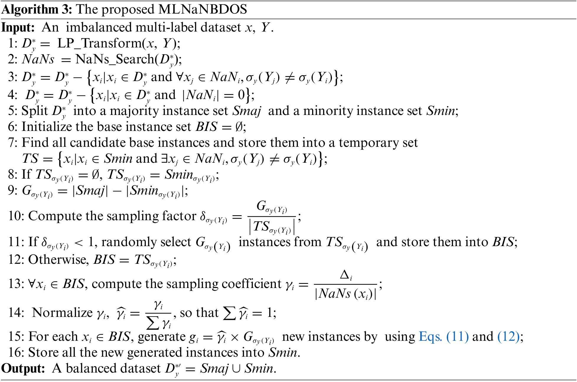
Algorithm 3 provides detailed information of MLNaNBDOS. In Step 1 of Algorithm 3, the LP_Transform algorithm (Algorithm 1) is used to convert the original multi-label dataset into a multi-class format. In Step 2, NaNs_Search (Algorithm 2) is employed to obtain natural neighbor information. Steps 3–4 involve the elimination of noise and outliers. Steps 5–12 focus on determining the base instance set. Steps 13–14 adaptively adjust the oversampling factor and sampling weights for the minority class samples. Step 15 generates new instances and precisely controls their categories. Finally, the dataset is balanced.

As previously mentioned, the time complexity of NaNs_Search is O(λ∗|X|∗log|X|) [17], where λ represents the natural neighbor eigenvalue, indicating the maximum number of natural neighbors for each instance. For MLNaNBDOS, besides invoking NaNs_Search, the time complexity for each step is either constant or linear. For example, linear traversal is performed in Steps 3 and 4 to identify noise or outliers. Therefore, the time complexity of MLNaNBDOS can be roughly estimated as O(λ∗|X|∗log|X|+λ∗|X|).

Fig. 2 illustrates the workflow of the MLNaNBDOS method. During the data preprocessing stage, noise and outliers are eliminated through the natural neighbor search strategy. In the oversampling stage (NaN oversampling), three steps are executed: selecting the base minority class sample instances, calculating sampling weights, generating new instances. Finally, the corresponding instance labels are generated to form the oversampled minority class samples, which are combined with the majority class samples to form the balanced training set.

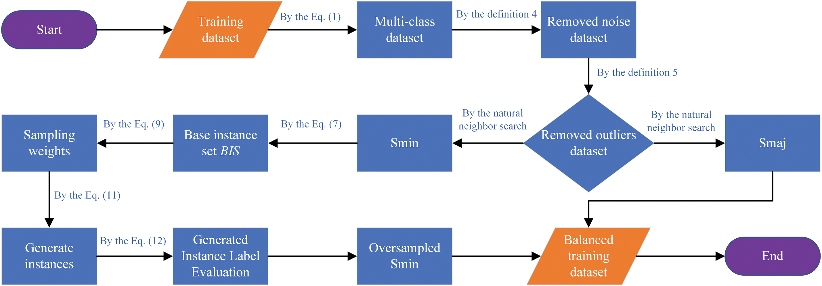
Figure 2: MLNaNBDOS flow chart

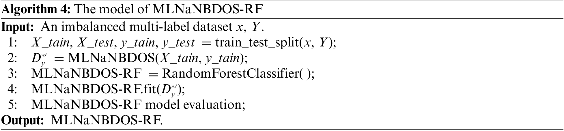
3.4 MLNaNBDOS-RF (Multi-Label Natural Neighbor Boundary Oversampling with Random Forest)

Generally, decision tree (DT) is suited for binary problems, while random forest (RF) and support vector machine (SVM) perform well in multi-class scenarios [22]. Due to RF’s outstanding performance with complex data and its ensemble approach, which provides strong anti-overfitting capabilities and robustness, RF is chosen as the classifier for the USC thermal power plant load deviation diagnosis model.

Reference [23] is an ensemble learning model that creates new training datasets by randomly sampling a samples from the training sample set D, and forms a random forest by generating a DTs. The classification result is obtained through a voting process among these DTs.

Algorithm 4 presents the pseudocode for integrating MLNaNBDOS with the RF classifier. Fig. 3 illustrates the workflow of the MLNaNBDOS-RF model.

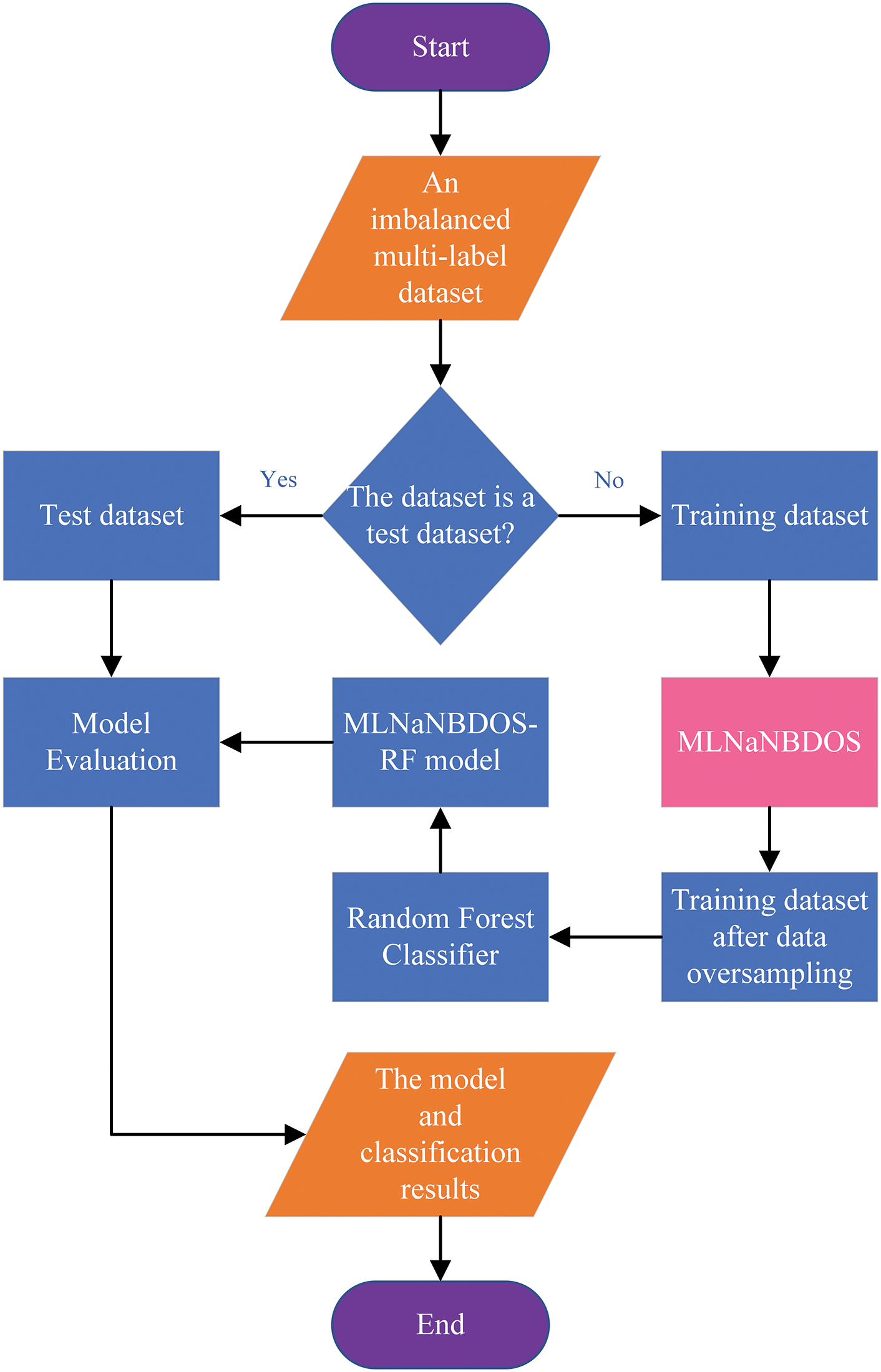
Figure 3: MLNaNBDOS-RF flow chart

4  Experiment

4.1 Dataset Description

To evaluate the classification performance of MLNaNBDOS on a dataset with class imbalance characteristics in USC unit load deviation, three sets of USC unit operational data under different AGC load commands were utilized as experimental datasets. The imbalance degree for each dataset is summarized in Table 1.

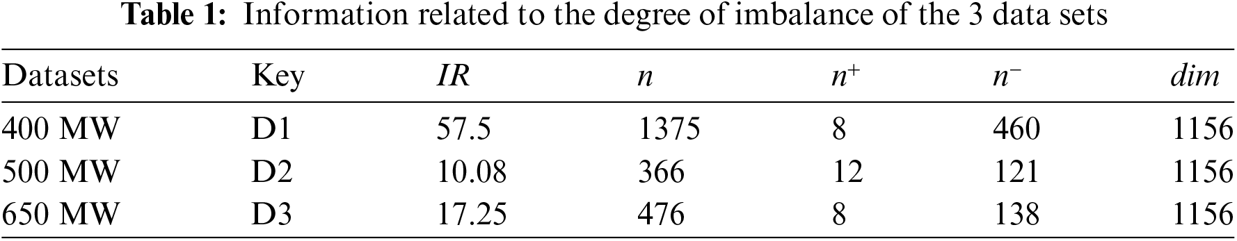
Where, n represents the total number of samples; n+ and n− denote the number of minority class (deviation data) samples and majority class (normal data) samples, respectively; dim refers to the number of features; and IR stands for imbalanced ratio, calculated as IR=n−/n+. For ease of reference, distinct Key values are used to represent the three different datasets.

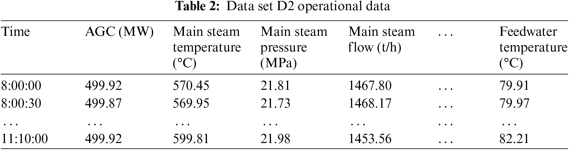
Each experimental dataset comprises 1156 features and 46 causal labels, with data collected at 30- s intervals. The feature data includes operational monitoring metrics such as temperature, pressure, current, voltage, vibration frequency, vibration displacement, emission concentration, and switch signal outputs from various equipment within the unit, encompassing the boiler, turbine, generator, and associated auxiliary equipment and systems. The label data pertains to the causal labels of the load deviation, where each label is assigned a value of “0” or “1”. Specifically, “0” indicates that the label is not a cause of load deviation, while “1” signifies that the label is a cause of load deviation. Table 2 presents a portion of the monitoring data from Dataset D2, with corresponding load deviation causal labels illustrated in Table 3.

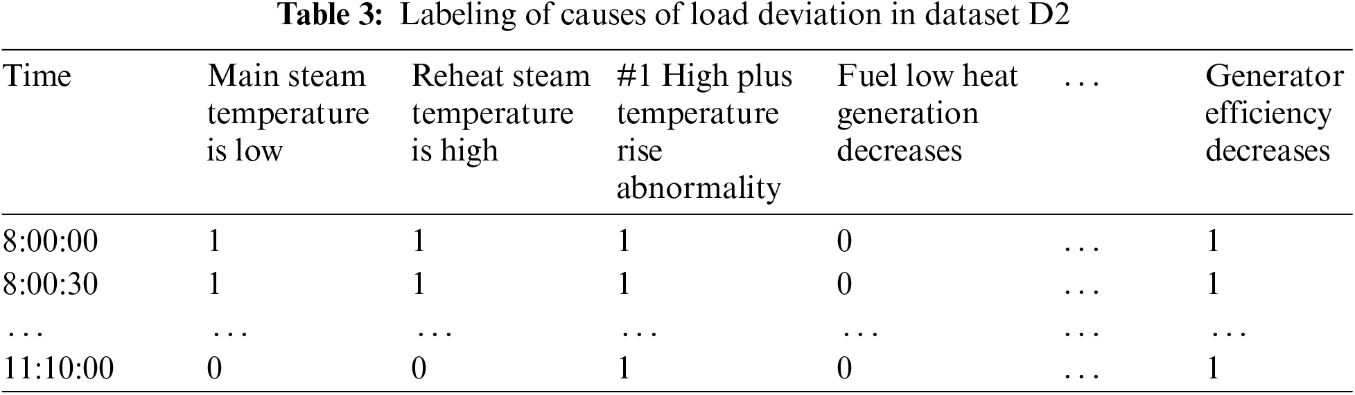
As shown in Table 3, multiple factors can concurrently contribute to insufficient load output in the unit. Moreover, there is a variation in the number of samples corresponding to each cause of insufficient load output, as detailed in Table 4. This disparity results in an imbalance in the sample count for different deviation causes, potentially impacting the classification performance of the load deviation diagnostic model.

4.2 Benchmark Model and Evaluation Metrics

4.2.1 Benchmark Model

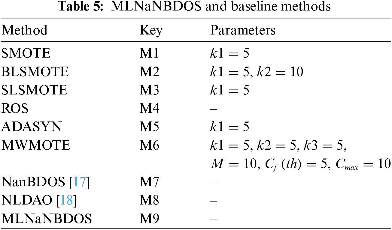
In this section, the classification performance of the MLNaNBDOS method is evaluated using datasets: D1, D2, and D3. For comparison, eight well-known oversampling methods are utilized, with specific parameter settings listed in Table 5. Safe level-SMOTE (SLSMOTE) [24], ADASYN [25], and MWMOTE [26] are implemented using the Smote-variants Python package [27]. SMOTE [28], Borderline-SMOTE (BLSMOTE) [29], and Random Over Sampler (ROS) [30] are implemented using the Imbalanced-learn Python package [31].

4.2.2 Evaluation Metrics

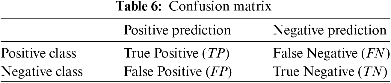
The evaluation of the proposed method is conducted using seven metrics: Micro-F1, Macro-F1, Micro-G-mean, Macro-G-mean, Micro-AUC, Macro-AUC, and Hamming Loss (HL) [32]. Both the F1 score and G-mean metrics are based on the confusion matrix presented in Table 6. A confusion matrix, also known as a likelihood table, an error matrix, or an error matrix, is a type of table especially suited for supervised learning to assess the performance of a classification model. In a confusion matrix, each row represents an actual category, each column represents a predicted category, and the value of each cell indicates the number of times a category was predicted to be another category. The confusion matrix visualizes which categories the classification model predicts accurately and in which categories there is confusion. The confusion matrix consists of four key elements, namely True Positive (TP), False Negative (FN), False Positive (FP), and True Negative (TN). FP is the number of instances of the negative category (majority) that are predicted as positive (minority) instances of the positive category number, and the TP, FN, and TN metrics are interpreted similarly.

The F1 score is the harmonic mean of Precision and Recall, focusing primarily on the minority class. The formulas for Micro-F1 and Macro-F1 are given in Eqs. (15) and (19), respectively.

Precisionmicro=∑TPi∑TPi+∑FPi(13)

Recallmicro=∑TPi∑TPi+∑FNi(14)

Micro−F1=2×Precisionmicro×RecallmicroPrecisionmicro+Recallmicro(15)

Precisioni=TPiTPi+FPi(16)

Recalli=TPiTPi+FNi(17)

F1i=2×Precisioni×RecalliPrecisioni+Recalli(18)

Macro−F1=1N∑i=1NF1i(19)

where N denotes the number of instance classes.

The G-mean is the geometric mean of Recall and Specificity, involving both minority and majority classes. The formulas for Micro-G-mean and Macro-G-mean are provided in Eqs. (22) and (26), respectively.

Recallmicro=∑TPi∑TPi+∑FNi(20)

Specificitymicro=∑TNi∑TNi+∑FPi(21)

Micro−G−mean=Recallmicro×Specificitymicro(22)

Recalli=TPiTPi+FNi(23)

Specificityi=TNiTNi+FPi(24)

G−meani=Recalli×Specificityi(25)

Macro−G−mean=1N∑i=1NG−meani(26)

Area Under Curve (AUC) refers to the area under the Receiver Operating Characteristic (ROC) curve, representing the probability that the classifier ranks a randomly chosen minority class instance higher than a randomly chosen majority class instance. Due to its insensitivity to class distribution, the AUC is particularly well-suited for addressing class imbalance issues.

Micro-AUC aggregates all classes into a binary classification problem and calculates the area under the ROC curve for true positive rate (TPR) vs. false positive rate (FPR) at various thresholds.

TPR=TPTP+FN(27)

FPR=FPFP+TN(28)

Macro-AUC is defined in Eq. (29).

Macro−AUC=1N∑i=1NAUCi(29)

Hamming Loss (HL) measures the misclassification rate of instance-label pairs. HL is defined in Eq. (30).

HL(h)=1p∑i=1p1q|h(xi)ΔYi|(30)

where ∆ denotes the symmetric difference between the predicted and actual labels of an instance.

All experiments were conducted on a personal computer with an R7-5800H CPU @ 3.20 GHz, 32 GB of memory, and running Windows 11.

4.3 Experimental Results and Analysis

4.3.1 Comparative Experiments of Different Oversampling Methods

To verify the distributional advantage of MLNaNBDOS in generating oversampled data, MLNaNBDOS will compare 8 oversampling methods on datasets D1~D3. The experimental results of the evaluation metrics for the 3 sets of datasets are shown in Tables 7–9, respectively, and the corresponding classification performance of the model is shown in Figs. 4–6, respectively. The confusion matrices in Figs. 4–6 have been normalized in the row direction, so the values in the cells indicate the probability that the model predicts the actual category or other categories.

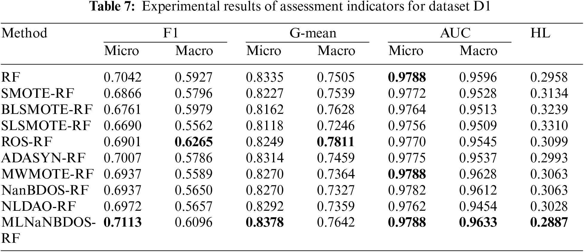
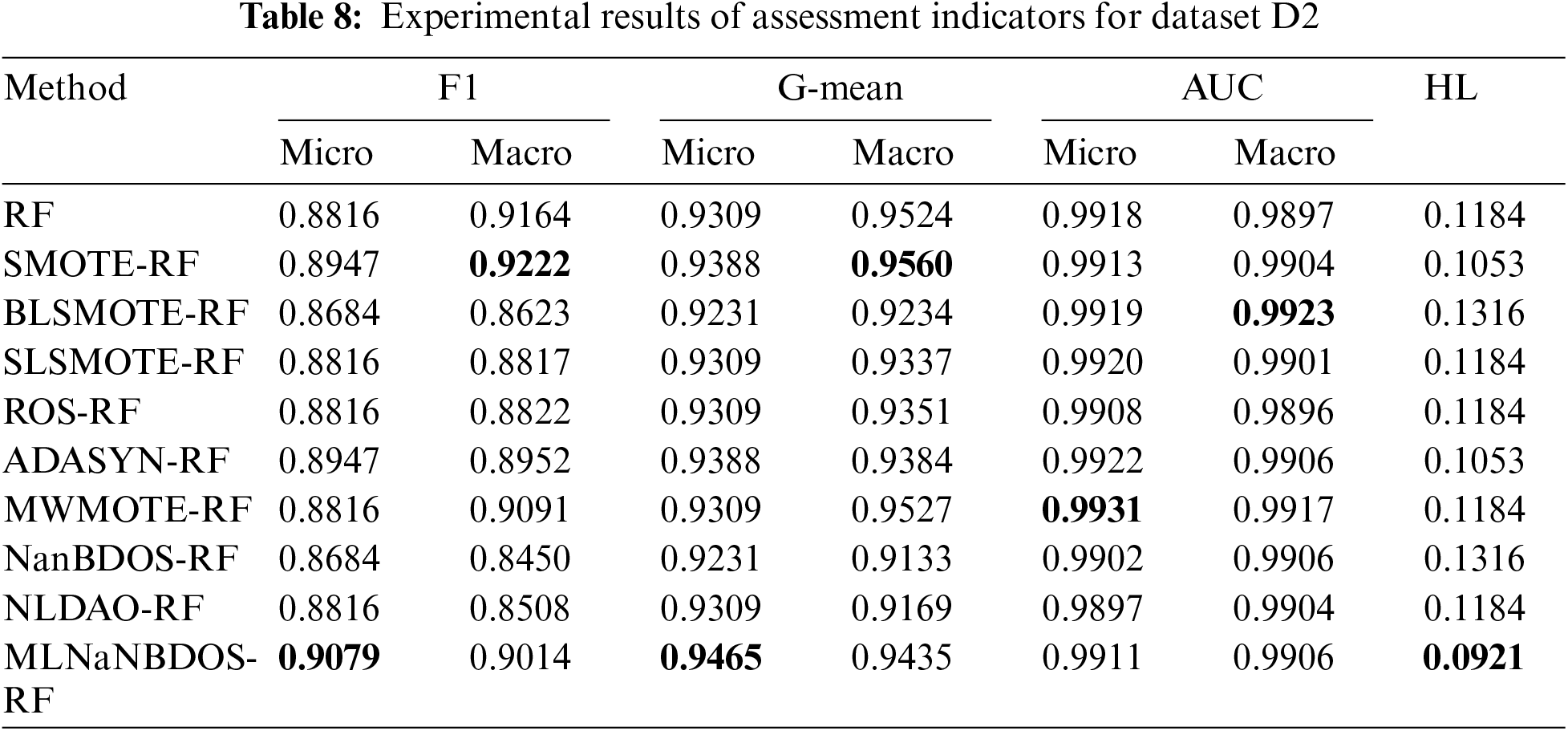
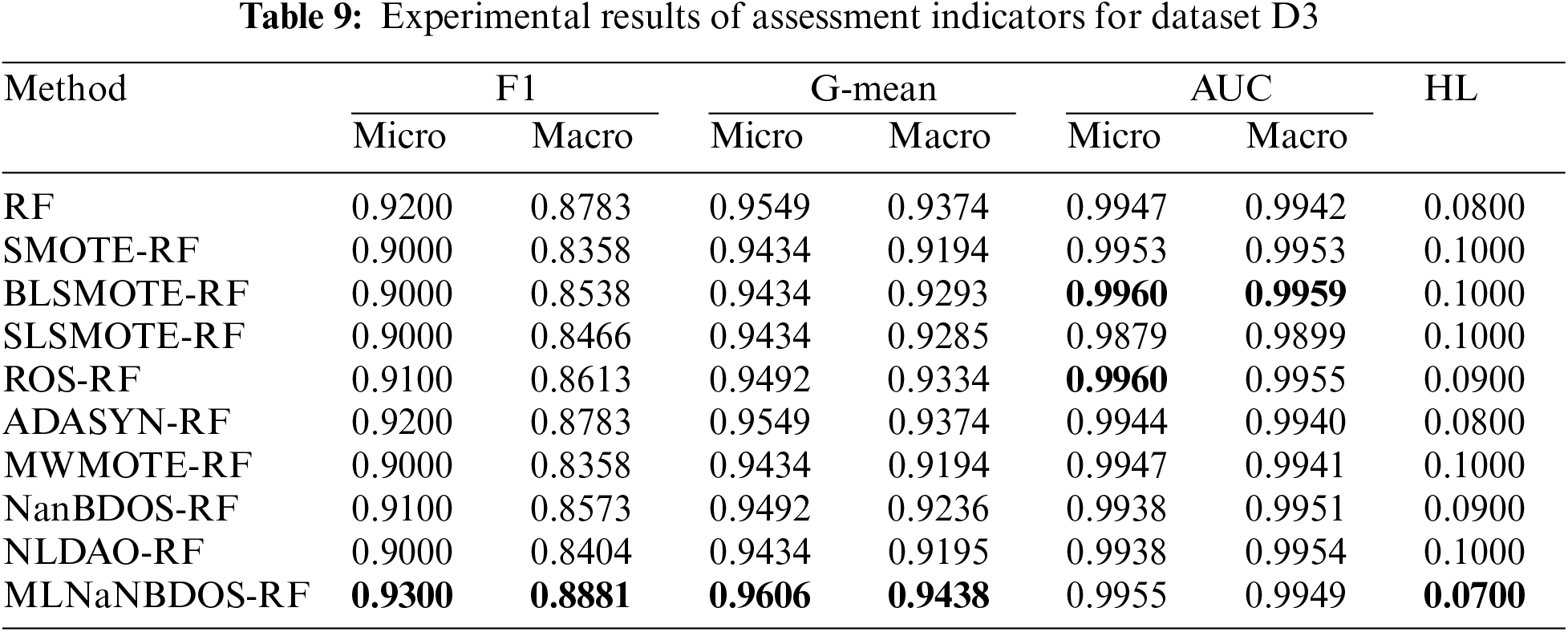
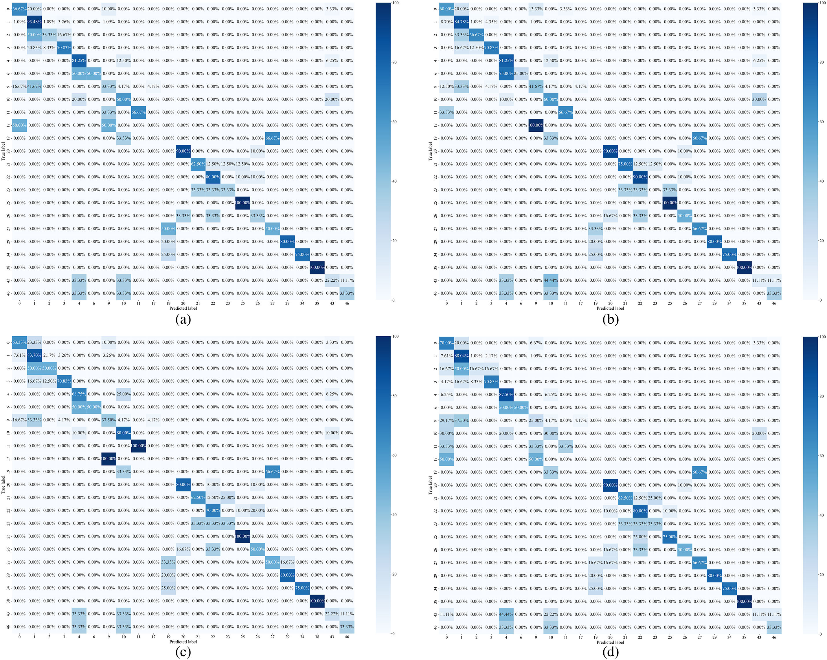
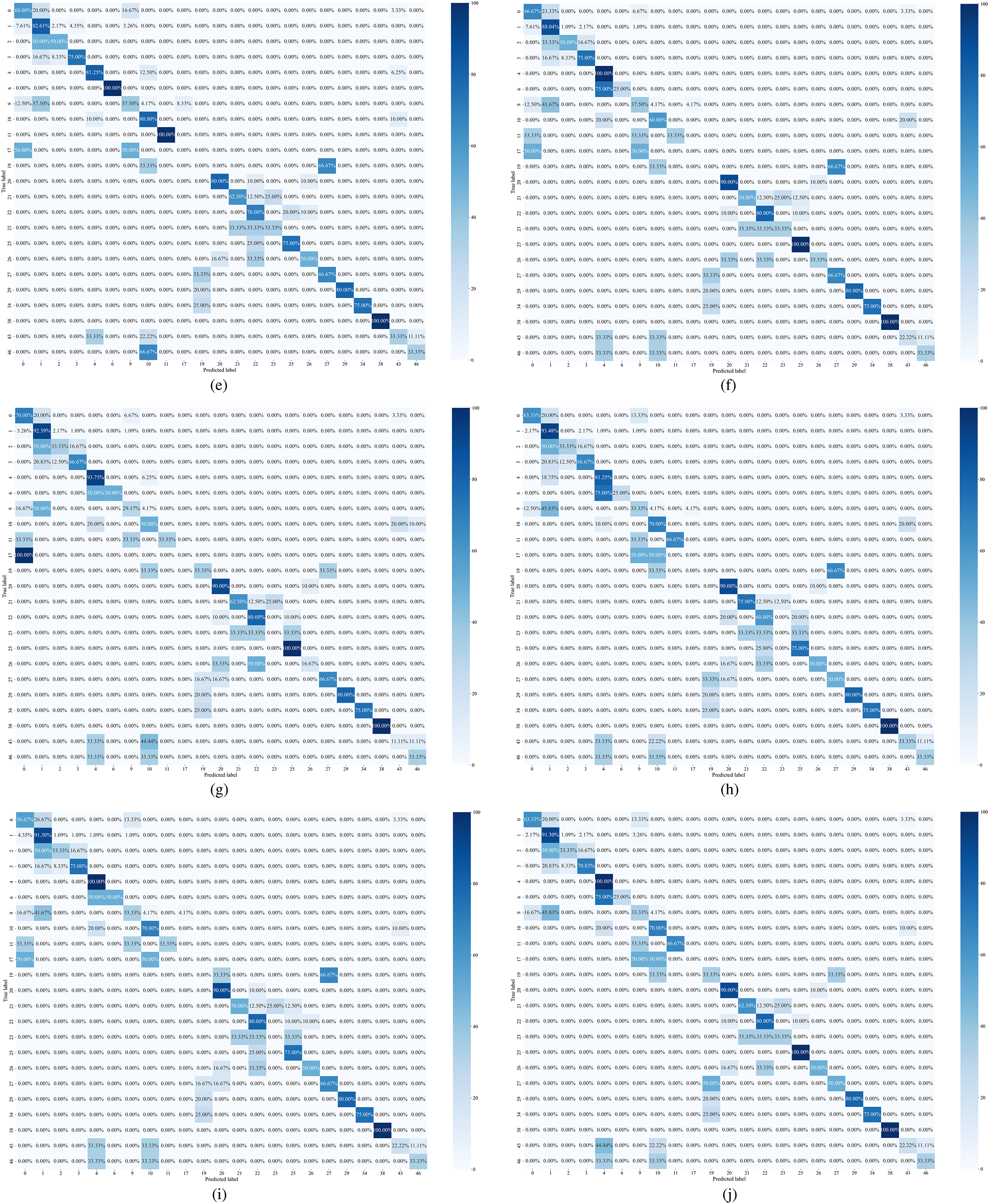
Figure 4: Confusion matrix for each oversampling method on dataset D1: (a) RF, (b) SMOTE-RF, (c) BLSMOTE-RF, (d) SLSMOTE-RF, (e) ROS-RF, (f) ADASYN-RF, (g) MWMOTE-RF, (h) NanBDOS-RF, (i) NLDAO-RF, (j) MLNaNBDOS-RF

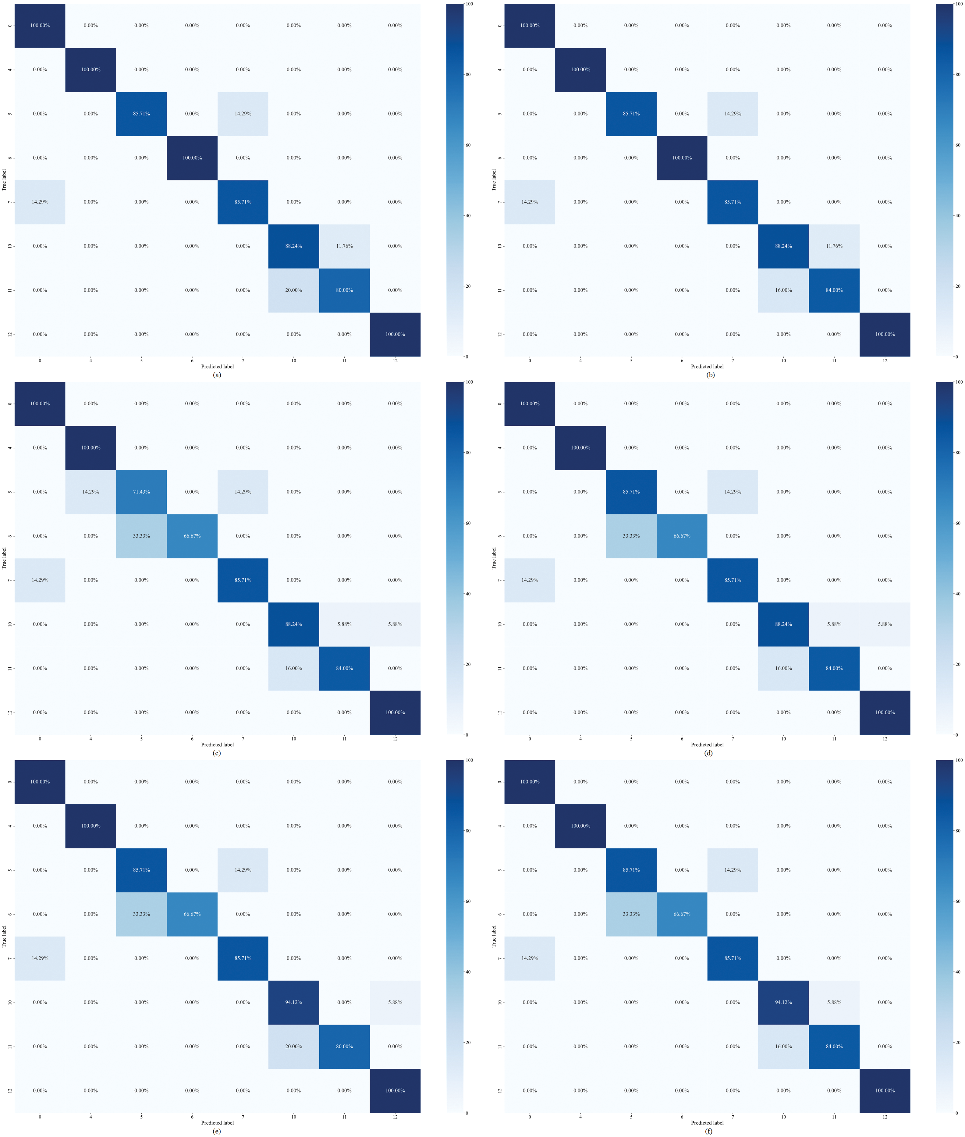
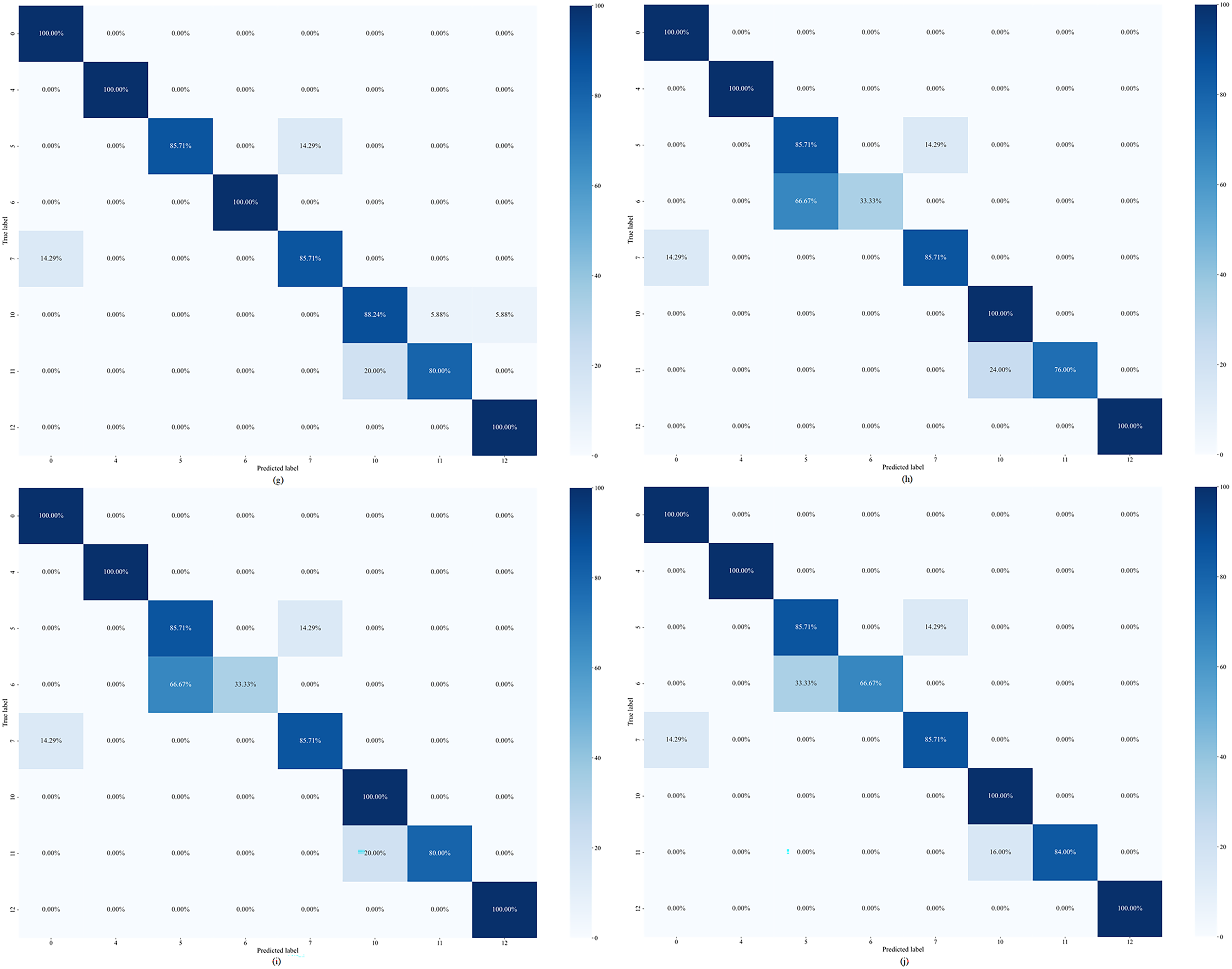
Figure 5: Confusion matrix for each oversampling method on dataset D2: (a) RF, (b) SMOTE-RF, (c) BLSMOTE-RF, (d) SLSMOTE-RF, (e) ROS-RF, (f) ADASYN-RF, (g) MWMOTE-RF, (h) NanBDOS-RF, (i) NLDAO-RF, (j) MLNaNBDOS-RF

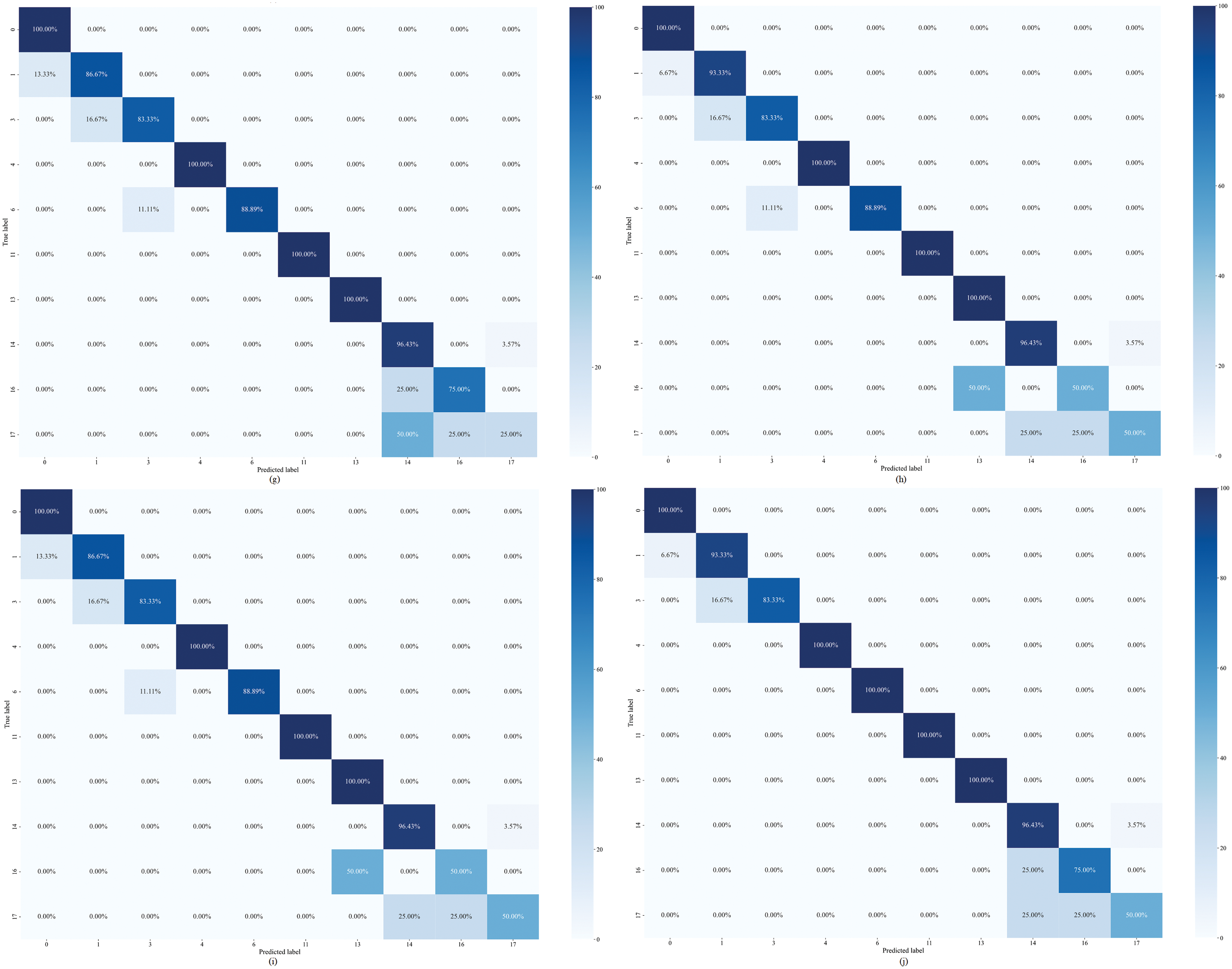
Figure 6: Confusion matrix for each oversampling method on dataset D3: (a) RF, (b) SMOTE-RF, (c) BLSMOTE-RF, (d) SLSMOTE-RF, (e) ROS-RF, (f) ADASYN-RF, (g) MWMOTE-RF, (h) NanBDOS-RF, (i) NLDAO-RF, (j) MLNaNBDOS-RF

Tables 4 and 7 present the performance evaluations for dataset D1, characterized by issues such as cylinder misalignment and low temperature before the main steam valve. The MLNaNBDOS achieved the best performance in Micro-F1, Micro-G-mean, Macro-AUC, and HL metrics, with scores of 0.7113, 0.8378, 0.9633, and 0.2887, respectively. The ROS exhibited the best performance in terms of Macro-F1 and Macro-G-mean, with scores of 0.6265 and 0.7811, respectively.

Among the methods with the highest Micro-AUC scores, including the benchmark RF, MWMOTE and MLNaNBDOS performed comparably to the original RF when classifying minority class samples characterized by low main steam flow, achieving a score of 0.9788. In contrast, other methods performed poorly. The highest Macro-AUC score was achieved by MLNaNBDOS, surpasssing other methods in classifying minority class samples, particularly those affected by cylinder misalignment and low temperature before the main steam valve.

Dataset D1 was transformed by the LP method to form 23 load deviation cause classes. The classification results of these load deviation cause classes by the basic classifier RF are shown in Fig. 4a. The classification results of these load deviation cause classes after oversampling and RF classification by nine oversampling methods are shown in Fig. 4b to j, respectively. From Fig. 4, MLNaNBDOS accurately predicts category 4 on top of RF accurately classifying category 25 and category 38, and further improves the probability of RF predicting category 19. SMOTE and BLSMOTE, although with outstanding global exploration capability, cause RF to accurately predict category 17 as category 9, which affects the RF classification performance. ROS possesses an excellent global exploration capability that improves RF categorization performance in category 6 and category 11, but like SLSMOTE and NanBDOS reduces RF’s probability of predicting category 25 by 25%. MWMOTE and ADASYN misclassify category 17 and accurately categorize category 4 on the basis of RF accurately predicting category 25 and category 38, respectively. NLDAO loses RF’s performance in categorizing category 25 and improves the ability to categorize category 4.

Based on Tables 4 and 8, for dataset D2, which is characterized by faults such as low reheating steam temperature and high-pressure regulator valve sticking, MLNaNBDOS performs best in terms of Micro-F1, Micro-G-mean, and HL, with values of 0.9079, 0.9465, and 0.0921, respectively. In Macro-F1 and Macro-G-mean, SMOTE excels, achieving values of 0.9222 and 0.9560, respectively. MWMOTE performs best in terms of Micro-AUC with a value of 0.9931, while BLSMOTE leads in Macro-AUC with a value of 0.9923.

As noted in Table 1, dataset D2 exhibits the least imbalanced and possesses the smallest sample size among the three datasets. With an equivalent number of features, fewer samples generally hinder classification performance. Thus, different methods emphasize various aspects when applied to dataset D2.

From a macro perspective, both SMOTE and BLSMOTE enhance global exploration capabilities by increasing the distribution density of the majority class samples within the kNN of the minority class samples. SMOTE focuses on macro-level precision and recall, whereas BLSMOTE emphasizes the occurrence probability of minority class samples.

Conversely, at a micro level, MLNaNBDOS further explores local information by examining the distribution density of minority class samples within the natural neighbors of minority class samples. MLNaNBDOS emphasizes micro-level precision and recall, as well as the misclassification rate of instance labels.

Dataset D2 was transformed by the LP method to form eight load deviation cause classes. The classification results of these load deviation cause classes by the basic classifier RF are shown in Fig. 5a. The classification results of these load deviation cause classes after oversampling and RF classification by nine oversampling methods are shown in Fig. 5b to j, respectively. As can be seen in Fig. 5, SMOTE, BLSMOTE, SLSMOTE, ADASYN, and MLNaNBDOS all improve the RF’s ability to categorize category 11 by 4%. ROS and ADASYN, while like BLSMOTE and SLSMOTE, cause the RF to lose 33.33% of its categorization performance in category 6, but improve its categorization performance in category 10 by 5.88%. NanBDOS, while causing RF to accurately categorize category 10, gives RF a 66.67% probability of predicting category 6 as category 5. On top of NanBDOS, NLDAO causes RF to improve its categorization performance in category 11 by 4%. On top of NLDAO, MLNaNBDOS further improves RF’s categorization performance in category 6 by 33.34%.

Tables 4 and 9 detail the performance metrics for dataset D3, which involves faults such as misaligned cylinders, low reheating steam temperature, and high-pressure regulator valve sticking, MLNaNBDOS excels in Micro-F1, Macro-F1, Micro-G-mean, Macro-G-mean, and HL, with respective values of 0.9300, 0.8881, 0.9606, 0.9438, and 0.0700. Both BLSMOTE and ROS perform best in terms of Micro-AUC, achieving 0.9960, while BLSMOTE leads in Macro-AUC with a value of 0.9959. Although MLNaNBDOS presents a slight 0.1% difference in AUC compared to BLSMOTE, it surpasses other methods in the remaining evaluation metrics.

Dataset D3 was transformed by the LP method to form 10 load deviation cause classes. The classification results of these load deviation cause classes by the basic classifier RF are shown in Fig. 6a. The classification results of these load deviation cause classes after oversampling and RF classification by nine oversampling methods are shown in Fig. 6b to j, respectively. As can be seen in Fig. 6, MLNaNBDOS increases the probability that the model RF predicts category 6 by 11.11%, allowing the model to further accurately categorize category 6 on top of its original categorization ability. BLSMOTE, SLSMOTE, and ROS add noise to the distribution of the category 1 and category 3 data, which affects the model’s predictions. SMOTE and MWMOTE give the model a 50% probability of misclassifying category 17 classified as category 14. Both NanBDOS and NLDAO reduce the probability of the model predicting category 16 by 25%.

Overall, across the three datasets, MLNaNBDOS consistently performs best in Micro-F1, Micro-G-mean, and HL, particularly in classifying faults such as misaligned cylinders, low reheating steam temperature, and high-pressure regulator valve sticking. The average values achieved are 0.8497, 0.9150, and 0.1503, respectively. MLNaNBDOS enhances the generation of new sample instances by accurately pairing new instance categories, thus effectively mitigating the creation of noise samples, and thereby improving both the robustness and accuracy of the classification model. Other methods, which inherit base instance categories during oversampling, tend to generate noise, thereby diminishing their classification performance and robustness across the three datasets. MLNaNBDOS demonstrates superior performance in micro-precision, micro-recall, micro-specificity, and instance label misclassification rate, proving to be the most effective in addressing class imbalance in the USC unit load deviation datasets.

4.3.2 Denoising Ablation Experiments

In order to verify the rationality and effectiveness of MLNaNBDOS in dealing with the noise problem, ablation experiments are conducted on this part. Model 1 denotes the use of NaN oversampling; Model 2 denotes the use of NaN oversampling and noise removal; Model 3 denotes the use of NaN oversampling and outlier removal; Model 4 denotes the use of NaN oversampling and control of new instance categories; Model 5 denotes the use of NaN oversampling, noise and outlier removal; Model 6 denotes the use of NaN oversampling, noise removal and control of new instance categories; and Model 7 denotes the use of NaN oversampling, removal of outliers, and control of new instance categories; MLNaNBDOS uses NaN oversampling, removal of noise and outliers, and control of new instance categories. The experimental results of the evaluation metrics for the 3 sets of datasets are shown in Tables 10–12, respectively, and the corresponding classification performance of the model is shown in Figs. 7–9, respectively.

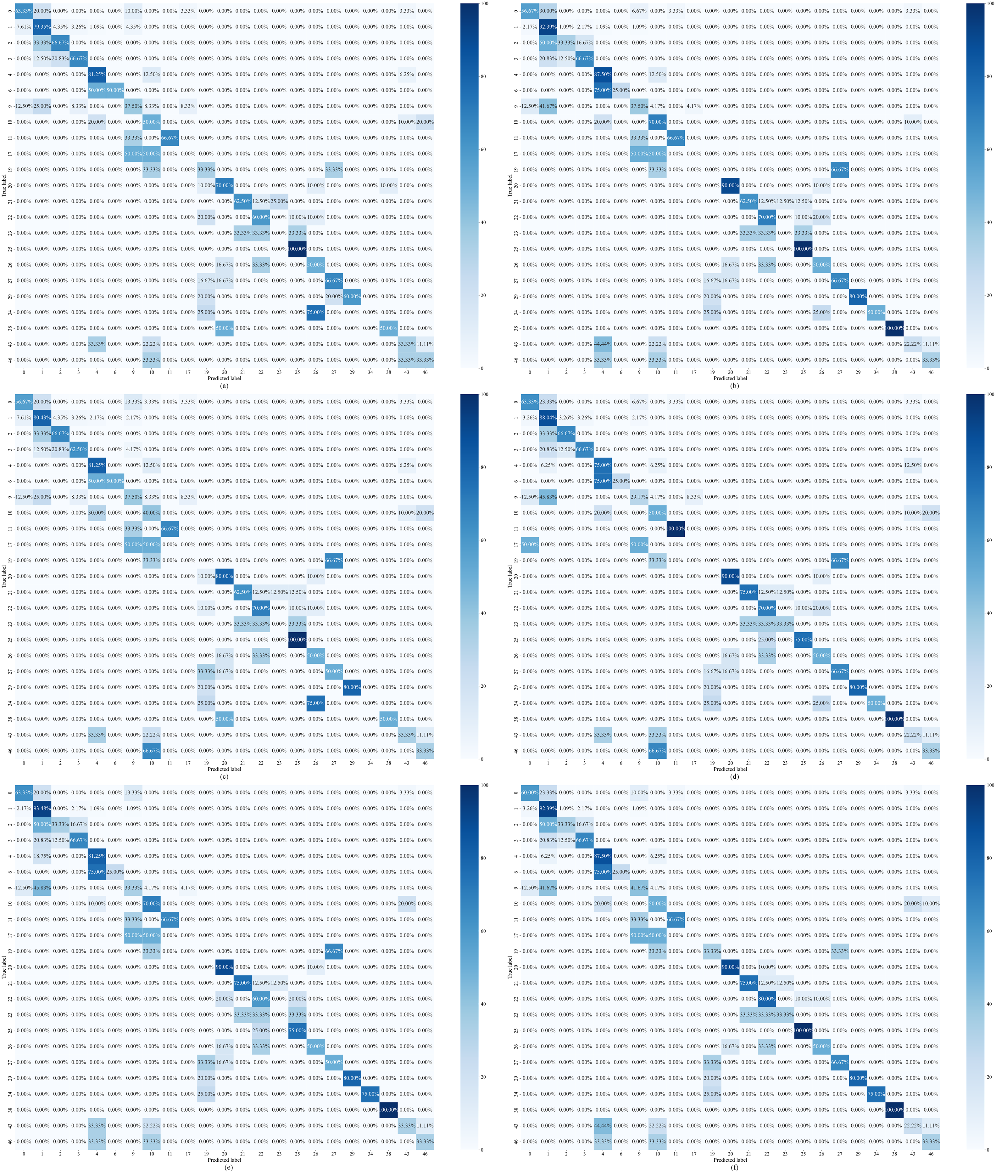
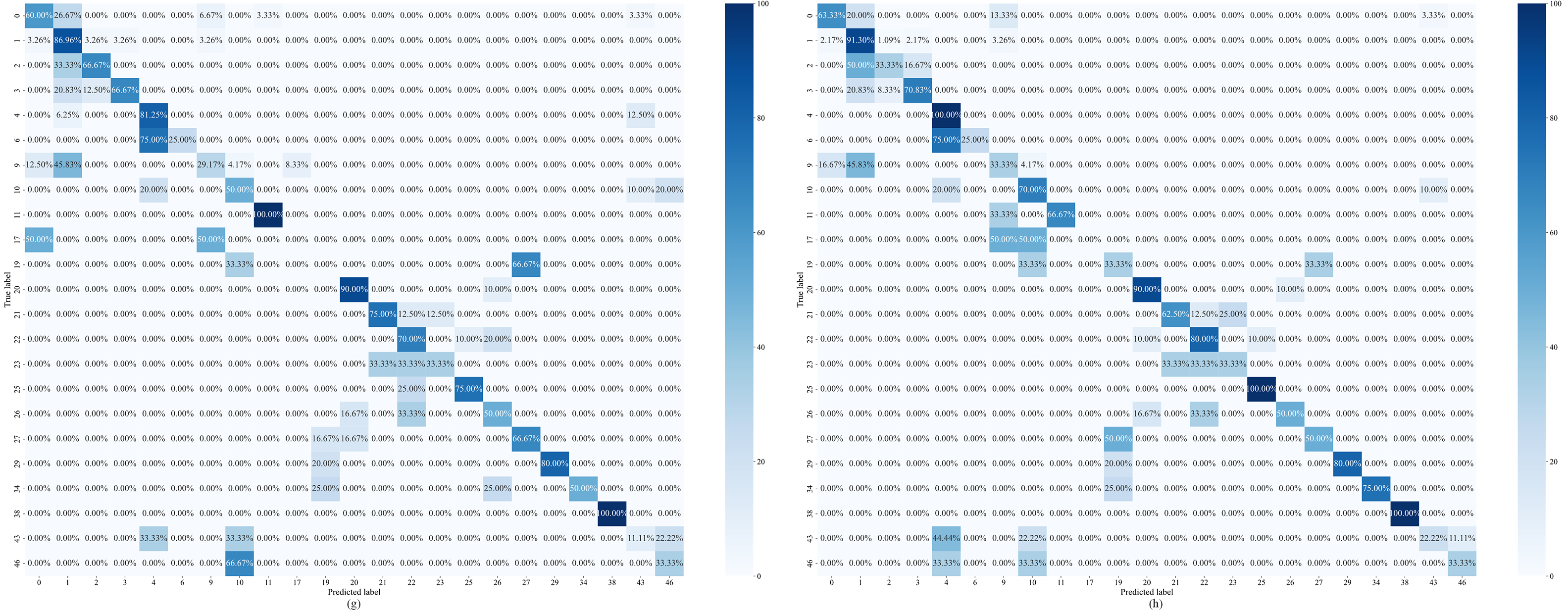
Figure 7: Confusion matrix for dataset D1 ablation experiments: (a) Model 1-RF, (b) Model 2-RF, (c) Model 3-RF, (d) Model 4-RF, (e) Model 5-RF, (f) Model 6-RF, (g) Model 7-RF, (h) MLNaNBDOS-RF

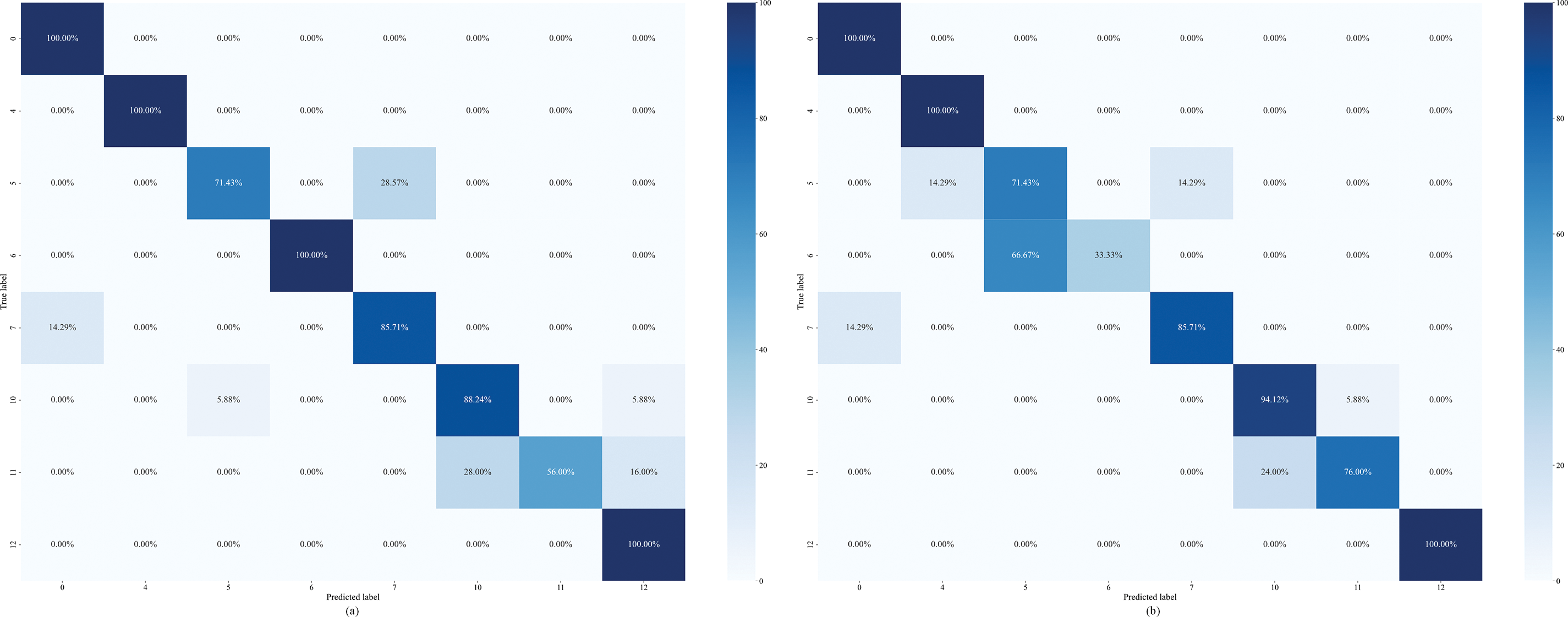
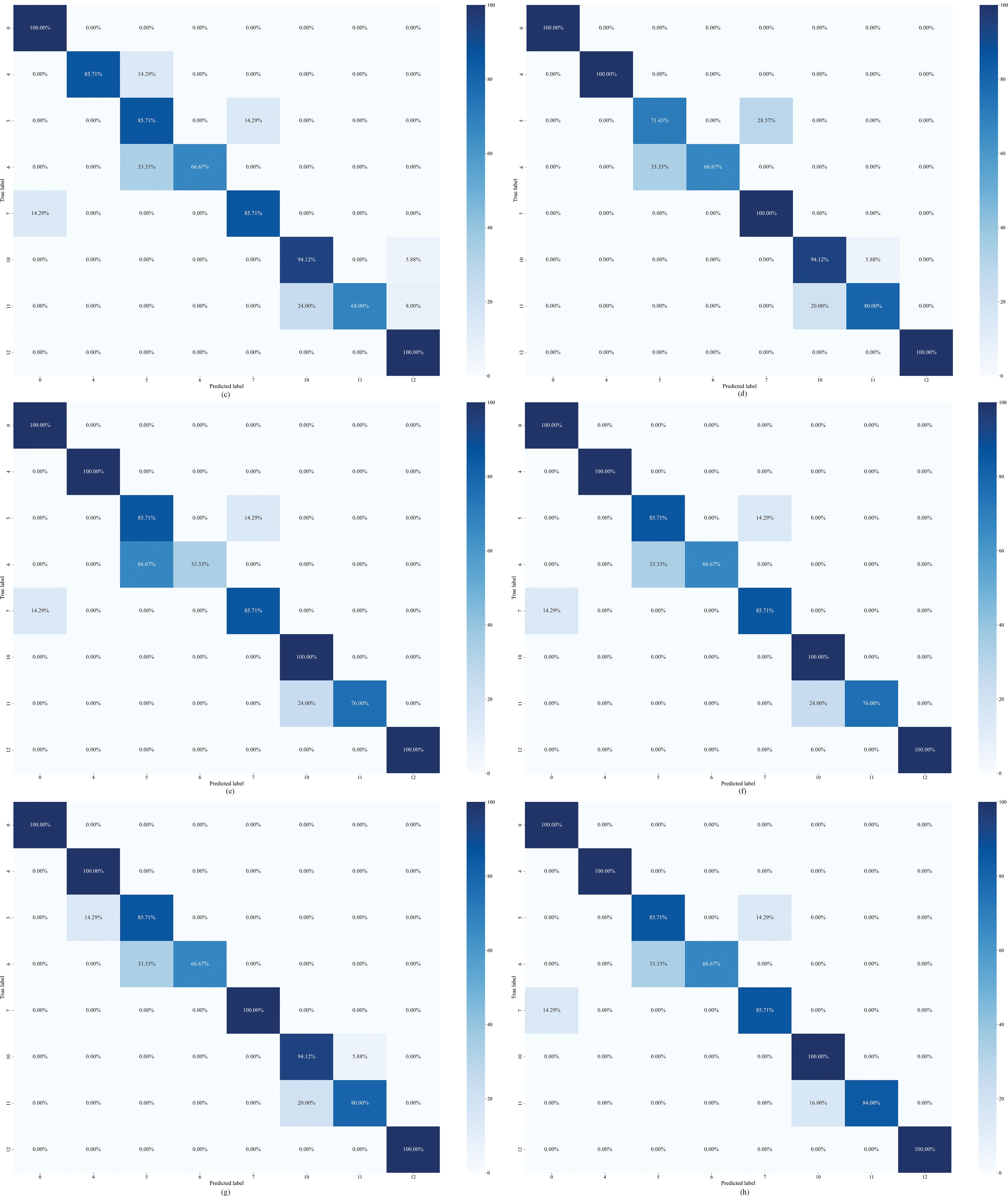
Figure 8: Confusion matrix for dataset D2 ablation experiments: (a) Model 1-RF, (b) Model 2-RF, (c) Model 3-RF, (d) Model 4-RF, (e) Model 5-RF, (f) Model 6-RF, (g) Model 7-RF, (h) MLNaNBDOS-RF

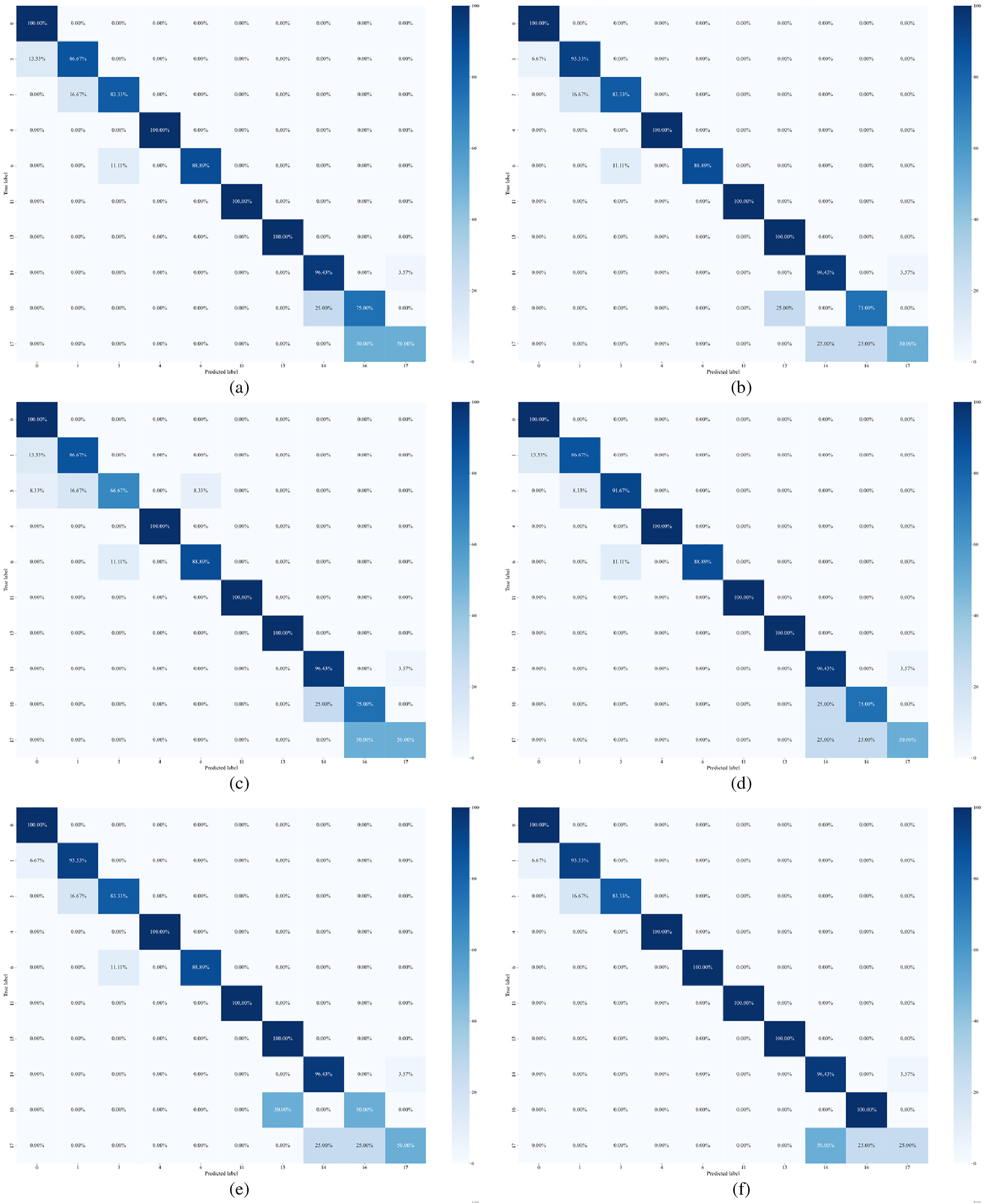
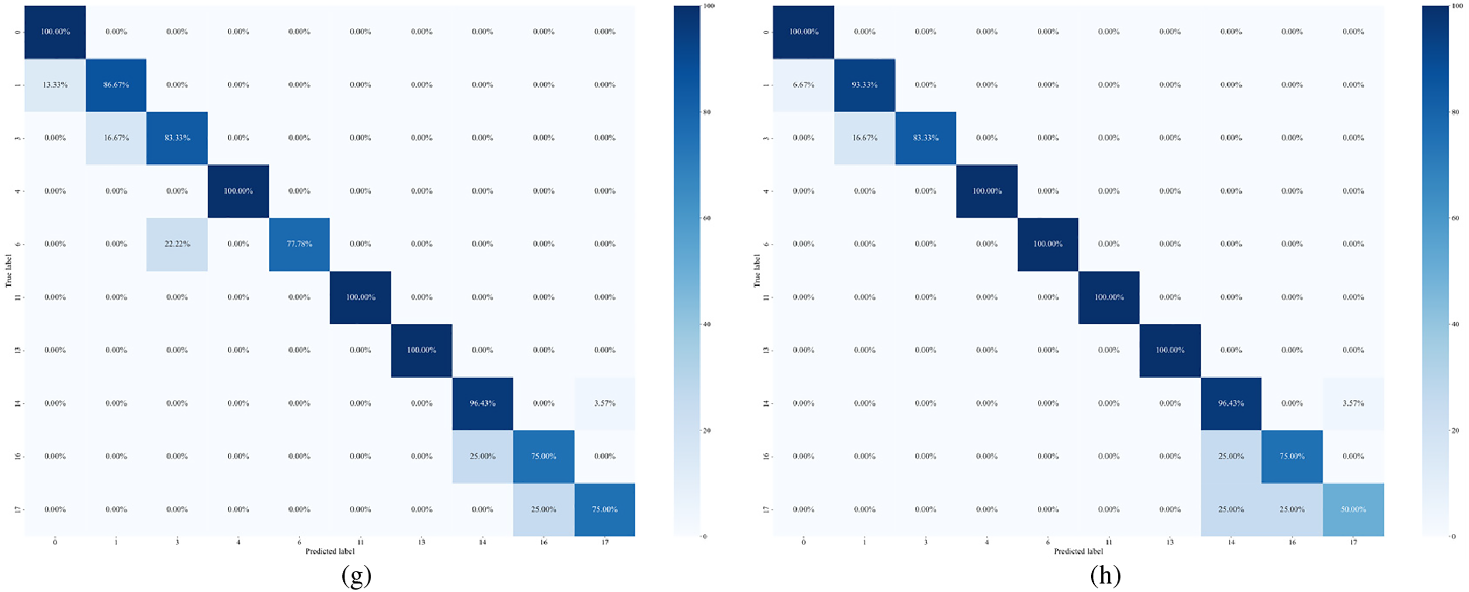
Figure 9: Confusion matrix for dataset D3 ablation experiments: (a) Model 1-RF, (b) Model 2-RF, (c) Model 3-RF, (d) Model 4-RF, (e) Model 5-RF, (f) Model 6-RF, (g) Model 7-RF, (h) MLNaNBDOS-RF

As can be seen from Table 10, MLNaNBDOS performs best in terms of F1, G-mean and HL, indicating that the RF classification ability can be effectively improved by the data preprocessing method that removes noise and outliers, as well as by controlling the new instance classes. As shown by the results of each evaluation index of Model 1 and Model 3, outlier detection performs poorly on dataset D1, indicating that the few classes of samples that are mistakenly detected as outliers are not able to form a natural neighbor relationship with other samples in the spatial distribution, which affects the RF classification performance. From the results of each evaluation index of Model 5 and Model 7, it can be seen that the use of removing noise or controlling new instance classes can improve RF classification performance and reduce the impact of noise and outlier detection on RF classification.

Dataset D1 was transformed by the LP method to form 23 load deviation cause classes. The classification results of these load deviation cause classes after Model 1–Model 7, MLNaNBDOS oversampling and RF classification, respectively, are shown in Fig. 7a–h. From Fig. 7a–d, removing noise causes RF to accurately categorize category 38, removing outliers causes RF to lose the performance of categorizing category 19, and controlling the new instance category causes RF to accurately categorize category 38 and category 11. From Fig. 7f–g, controlling the new instance category after removing noise or outliers causes RF to improve its categorization ability in category 23 by 33.33%. From Fig. 7h, the denoising effect of the combination of removing noise, removing outliers, and controlling new instance categories makes RF accurately categorize category 4.

As can be seen in Table 11, controlling for new instance categories excels on dataset D2, and in particular, the combination of removing outliers and controlling for new instance categories resulted in the best representation of RF on Macro-F1, Macro-G-mean, and AUC. The combination of removing noise, removing outliers, and controlling for new instance categories resulted in the lowest HL score and the best overall categorization for RF.

Dataset D2 was transformed by the LP method to form 8 load deviation cause classes. The classification results of these load deviation cause classes after Model 1–Model 7, MLNaNBDOS oversampling and RF classification, respectively, are shown in Fig. 8a–h. As can be seen in Fig. 8, while removing noise, removing outliers and controlling the new instance category all degrade the RF in terms of classification performance for category 6, controlling the new instance category results in the largest increase in the RF’s ability to classify in category 11 of up to 24% and to accurately classify in category 7. This suggests that controlling the new instance category has the best results in terms of the ability to denoise samples from both category 11 and category 7.

As can be seen from Table 12, outlier detection is ineffective on dataset D3, lowering MLNaNBDO S’s score on AUC while improving RF’s Macro-F1 score by 1.13%. This suggests that on dataset D3, outlier detection excludes some of the valuable minority class samples, making RF slightly less effective in predicting minority class sample performance.

Dataset D3 was transformed by the LP method to form 10 load deviation cause classes. The classification results of these load deviation cause classes after Model 1~Model 7, MLNaNBDOS oversampling and RF classification, respectively, are shown in Fig. 9a–h. As can be seen from Fig. 9, on dataset D3, the removal of outliers reduces the classification ability of RF in category 3 by 16.66%, and improves the misclassification ability in category 0 and category 6 by 8.33%, respectively. This indicates that the few class samples removed are similar to category 0 and category 6 in spatial distribution and cannot form a natural neighbor relationship with category 3 samples, which affects the outlier detection effect. In addition, removing noise improves RF’s categorization ability in category 1 by 6.66%, and controlling for new instance categories improves RF’s categorization ability in category 3 by 8.34%. The combination of removing noise, removing outliers, and controlling new instance categories improves RF’s ability to classify category 1 by 6.66% and accurately classifies category 6.

Combining 3 sets of datasets, the combination of removing noise, removing outliers and controlling new instance categories effectively removes the original noise, while avoiding new noise samples generation on new instance sample generation, thus improving RF classification ability.

5  Conclusion

This study addresses the issue of class imbalance prevalent in datasets concerning supercritical coal-fired power plant unit load deviation. A diagnostic method for load deviation in supercritical units is introduced, utilizing the multi-label natural neighbor boundary oversampling technique (MLNaNBDOS). This method is crafted to optimize and enhance diagnostic performance. The primary contributions of MLNaNBDOS are as follows:

1) Multidimensional Label Oversampling Strategy. MLNaNBDOS constructs the load deviation causes of coal-fired power units as binary multi-label relationships. By introducing the label power set method, it retains complex inter-data correlations, thereby enhancing the flexibility and applicability of traditional binary classification oversampling strategies for multi-label classification problems.

2) Intelligent Adjustment of Oversampling Factors. Addressing the poor performance of traditional binary classification oversampling techniques in multi-class environments, MLNaNBDOS utilizes a natural neighbor search strategy to adaptively adjust the oversampling factors and weights. This improves the accuracy of oversampling for each class and enhances the generalization ability of the oversampling algorithm in multi-class scenarios.

3) Precise Control of New Instance Categories. To overcome potential noise issues introduced by traditional oversampling methods during new instance generation, MLNaNBDOS leverages natural neighbor information to adaptively pair new instance categories. By dynamically evaluating the similarity between new instances and natural neighbors using random factors, MLNaNBDOS precisely controls the new instance generation process, effectively diminishing noise samples and thereby improving the robustness and accuracy of the classification model.

The experimental results underscore the exceptional performance of MLNaNBDOS across critical evaluation metrics. For three significantly imbalanced datasets concerning coal-fired power unit load deviations, MLNaNBDOS achieved average values of 0.8497 in Micro-F1, 0.9150 in Micro-G-mean, and 0.1503 in Hamming Loss. Specifically, in terms of micro-precision, recall, specificity, and instance-label misclassification rates, MLNaNBDOS significantly outperforms other comparative methods, validating its efficacy and superiority in practical applications.

Given the urgent demand for automation and intelligent maintenance within smart power plants, the MLNaNBDOS diagnostic model for ultra-supercritical unit load deviations provides decision support for plant operators and maintenance teams. While this model has demonstrated robust capabilities, it requires further refinement at a macro level, especially in enhancing the prediction accuracy for minority class occurrences. Future research will focus on deepening theoretical foundations and exploring more efficient base instance selection strategies. Such advancements are expected to significantly improve macro classification capability, thereby further solidifying and enhancing the overall performance of the ultra-supercritical unit load fault diagnosis model.

Acknowledgement: The authors would like to acknowledge the constructive remarks by worthy reviewers that led to this revised article.

Funding Statement: This work was supported by the National Natural Science Foundation of China (Grant No. 62173050), Shenzhen Municipal Science and Technology Innovation Committee (Grant No. KCXFZ20211020165004006), Natural Science Foundation of Hunan Province of China (Grant No. 2023JJ30051), Hunan Provincial Graduate Student Research Innovation Project (Grant No. QL20230214), Major Scientific and Technological Innovation Platform Project of Hunan Province (2024JC1003), and Hunan Provincial University Students’ Energy Conservation and Emission Reduction Innovation and Entrepreneurship Education Center (Grant No. 2019-10).

Author Contributions:: The authors confirm contribution to the paper as follows: study conception and design: Mingzhu Tang, Yujie Huang; data collection: Mingzhu Tang; analysis and interpretation of results: Yujie Huang, Dongxu Ji, Hao Yu; draft manuscript preparation: Yujie Huang, Hao Yu. All authors reviewed the results and approved the final version of the manuscript.

Availability of Data and Materials: Due to the nature of this research, participants of this study did not agree for their data to be shared publicly, so supporting data is not available.

Ethics Approval: Not applicable.

Conflicts of Interest: The authors declare no conflicts of interest to report regarding the present study.

References

1. Zhang Q, Dong J, Chen H, Feng F, Xu G, Wang X, et al. Dynamic characteristics and economic analysis of a coal-fired power plant integrated with molten salt thermal energy storage for improving peaking capacity. Energy. 2024;290:130132. doi:10.1016/j.energy.2023.130132. [Google Scholar] [CrossRef]

2. Baranda M, Mayo C, Diaz R, Rodriguez R, Pérez FJ. Comparative environmental assessment of coated ferritic steels suited to steam turbines of coal-fired supercritical and ultra-supercritical power plants. J Cleaner Prod. 2024;443:141226. doi:10.1016/j.jclepro.2024.141226. [Google Scholar] [CrossRef]

3. Opriş I, Cenuşă V-E, Norişor M, Darie G, Alexe F-N, Costinaş S. Parametric optimization of the thermodynamic cycle design for supercritical steam power plants. Energy Convers Manage. 2020;208:112587. doi:10.1016/j.enconman.2020.112587. [Google Scholar] [CrossRef]

4. Zhou J, Zhang W. Coal consumption prediction in thermal power units: a feature construction and selection method. Energy. 2023;273:126996. doi:10.1016/j.energy.2023.126996. [Google Scholar] [CrossRef]

5. Fan H, Su Z-G, Wang P-H, Lee KY. A dynamic nonlinear model for a wide-load range operation of ultra-supercritical once-through boiler-turbine units. Energy. 2021;226:120425. doi:10.1016/j.energy.2021.120425. [Google Scholar] [CrossRef]

6. Xie Y, Liu J-Z, Zeng D-L, Hu Y, Zhu Y-S, Li R-L. A dynamic mathematical model used for controller design of a supercritical once-through boiler-turbine unit in all load conditions. Appl Therm Eng. 2024;248(7):123139. doi:10.1016/j.applthermaleng.2024.123139. [Google Scholar] [CrossRef]

7. Zhou J, Zhang L, Zhu L, Zhang W. A data-driven operating improvement method for the thermal power unit with frequent load changes. Appl Energy. 2024;354:122195. doi:10.1016/j.apenergy.2023.122195. [Google Scholar] [CrossRef]

8. Huang C, Li Z. Data-driven modeling of ultra-supercritical unit coordinated control system by improved transformer network. Energy. 2023;266:126473. doi:10.1016/j.energy.2022.126473. [Google Scholar] [CrossRef]

9. Chen C, Liu M, Li M, Wang Y, Wang C, Yan J. Digital twin modeling and operation optimization of the steam turbine system of thermal power plants. Energy. 2024;290:129969. doi:10.1016/j.energy.2023.129969. [Google Scholar] [CrossRef]

10. Tang M, Liang Z, Ji D, Yi J, Peng Z, Huang Y, et al. Inadequate load output diagnosis of ultra-supercritical thermal power units based on MIWOA multi-label random forest. Appl Therm Eng. 2023;227:120386. doi:10.1016/j.applthermaleng.2023.120386. [Google Scholar] [CrossRef]

11. Li S, Peng Y, Shen Y, Zhao S, Shao H, Bin G, et al. Rolling bearing fault diagnosis under data imbalance and variable speed based on adaptive clustering weighted oversampling. Reliab Eng Syst Saf. 2024;244:109938. doi:10.1016/j.ress.2024.109938. [Google Scholar] [CrossRef]

12. Hou Y, Wang Q, Zhou K, Zhang L, Tan T. Integrated machine learning methods with oversampling technique for regional suitability prediction of waste-to-energy incineration projects. Waste Manage. 2024;174:251–62. doi:10.1016/j.wasman.2023.12.006. [Google Scholar] [PubMed] [CrossRef]

13. Roy SD, Debbarma S, Guerrero JM. A data-driven algorithm to detect false data injections targeting both frequency regulation and market operation in power systems. Int J Electr Power Energy Syst. 2022;143:108409. doi:10.1016/j.ijepes.2022.108409. [Google Scholar] [CrossRef]

14. Wang W, Yang L, Yang J, Zhang J, Tang D, Liu T. NMNN: Newtonian Mechanics-based Natural Neighbor algorithm. Inf Sci. 2024;681:121200. doi:10.1016/j.ins.2024.121200. [Google Scholar] [CrossRef]

15. Li J, Zhu Q, Wu Q, Fan Z. A novel oversampling technique for class-imbalanced learning based on SMOTE and natural neighbors. Inf Sci. 2021;565:438–55. doi:10.1016/j.ins.2021.03.041. [Google Scholar] [CrossRef]

16. Li J, Zhu Q, Wu Q, Zhang Z, Gong Y, He Z, et al. SMOTE-NaN-DE: addressing the noisy and borderline examples problem in imbalanced classification by natural neighbors and differential evolution. Knowl-Based Syst. 2021;223:107056. doi:10.1016/j.knosys.2021.107056. [Google Scholar] [CrossRef]

17. Leng Q, Guo J, Jiao E, Meng X, Wang C. NanBDOS: adaptive and parameter-free borderline oversampling via natural neighbor search for class-imbalance learning. Knowl-Based Syst. 2023;274:110665. doi:10.1016/j.knosys.2023.110665. [Google Scholar] [CrossRef]

18. Wang W, Yang L, Zhang J, Yang J, Tang D, Liu T. Natural local density-based adaptive oversampling algorithm for imbalanced classification. Knowl-Based Syst. 2024;295:111845. doi:10.1016/j.knosys.2024.111845. [Google Scholar] [CrossRef]

19. Tarekegn AN, Giacobini M, Michalak K. A review of methods for imbalanced multi-label classification. Pattern Recognit. 2021;118:107965. doi:10.1016/j.patcog.2021.107965. [Google Scholar] [CrossRef]

20. Guan H, Zhao L, Dong X, Chen C. Extended natural neighborhood for SMOTE and its variants in imbalanced classification. Eng Appl Artif Intell. 2023;124:106570. doi:10.1016/j.engappai.2023.106570. [Google Scholar] [CrossRef]

21. Zhang A, Yu H, Huan Z, Yang X, Zheng S, Gao S. SMOTE-RkNN: a hybrid re-sampling method based on SMOTE and reverse k-nearest neighbors. Inf Sci. 2022;595:70–88. doi:10.1016/j.ins.2022.02.038. [Google Scholar] [CrossRef]

22. García-Pedrajas NE, Cuevas-Muñoz JM, Cerruela-García G, de Haro-García A. A thorough experimental comparison of multilabel methods for classification performance. Pattern Recognit. 2024;151:110342. doi:10.1016/j.patcog.2024.110342. [Google Scholar] [CrossRef]

23. Xie A, An L, Chen H, Xue X, Xu G. Performance optimization of the air-cooling system in a coal-fired power unit based on intelligent algorithms. Appl Therm Eng. 2023;230:120791. doi:10.1016/j.applthermaleng.2023.120791. [Google Scholar] [CrossRef]

24. Qin J, Yang D, Zhou B, Sun Y. Semi-supervised variational bi-directional sampling on multi-class imbalanced electric power data for fault diagnosis. Int J Electr Power Energy Syst. 2024;155:109512. doi:10.1016/j.ijepes.2023.109512. [Google Scholar] [CrossRef]

25. He Y, Zhou J, Cao C, Wang S, Fu H. Detection of electricity theft based on Minimal Gated Memory network combined adaptive synthesis sampling and decision tree. Sustain Energy Grids Netw. 2024;39:101415. doi:10.1016/j.segan.2024.101415. [Google Scholar] [CrossRef]

26. Yuan Y, Wei J, Huang H, Jiao W, Wang J, Chen H. Review of resampling techniques for the treatment of imbalanced industrial data classification in equipment condition monitoring. Eng Appl Artif Intell. 2023;126(2):106911. doi:10.1016/j.engappai.2023.106911. [Google Scholar] [CrossRef]

27. Koziarski M. Potential anchoring for imbalanced data classification. Pattern Recognit. 2021;120(4):108114. doi:10.1016/j.patcog.2021.108114. [Google Scholar] [CrossRef]

28. Allal Z, Noura HN, Salman O, Chahine K. Leveraging the power of machine learning and data balancing techniques to evaluate stability in smart grids. Eng Appl Artif Intell. 2024;133(21):108304. doi:10.1016/j.engappai.2024.108304. [Google Scholar] [CrossRef]

29. Smiti S, Soui M. Bankruptcy prediction using deep learning approach based on borderline SMOTE. Inf Syst Front. 2020;22(5):1067–83. doi:10.1007/s10796-020-10031-6. [Google Scholar] [CrossRef]

30. Klikowski J, Woźniak M. Deterministic sampling classifier with weighted bagging for drifted imbalanced data stream classification. Appl Soft Comput. 2022;122:108855. doi:10.1016/j.asoc.2022.108855. [Google Scholar] [CrossRef]

31. Gantert L, Zeffiro T, Sammarco M, Campista MEM. Multiclass classification of faulty industrial machinery using sound samples. Eng Appl Artif Intell. 2024;136:108943. doi:10.1016/j.engappai.2024.108943. [Google Scholar] [CrossRef]

32. Tang J, Yi Q, Fu S, Tian Y. Incomplete multi-view learning: review, analysis, and prospects. Appl Soft Comput. 2024;153:111278. doi:10.1016/j.asoc.2024.111278. [Google Scholar] [CrossRef]

Appendix A