Thermodynamic Analysis of Marangoni Convection in Magnetized Nanofluid

1  Introduction

Drying of silicon wafers, electron beam melting, growth of crystals, and convection cells involve surface tension gradient-induced flows. Such flows are called Marangoni convective flows in which the change in surface tension can be brought about by gradients in temperature (called thermal Marangoni convection) or solute (called solutal Marangoni convection) [1]. The Marangoni flow is undesirable in crystal growth and thermal Marangoni convection is dominant in semiconductor melts of Silicon [2]. At the interface, the surface tension (σ) is modeled such that it varies linearly with temperature as given below [3]:

σ=σ∞−σT(T−T∞)(1)

where, σT=−dσdT>0 and σ∞ is the surface tension at T∞. The steady flow of liquids in slots considering thermal Marangoni convection was analyzed by Sen et al. [4]. The deflection of the liquid-gas interface due to the considered pressure gradient is studied. Chamkha et al. [5] explored the mixed Marangoni flow by considering gravitational and pressure gradient effects in a small fluid flayer. The substantial impact of the mixed convective parameter on heat transport was concluded. Khan et al. [6] used the cylindrical coordinate system to analyze the thermal Marangoni flow with dissipative forces and an irregular heat source. Moreover, the entropy generated in the system was analyzed, and concluded a boost in entropy generation due to the Marangoni aspect. The optimized heat transport rate in the Marangoni boundary layer flow of a hybrid nanomaterial was reported by Mackolil et al. [7]. The radiated thermal profile was studied in detail along with an exponentially varying heat source and a magnetism that is inclined. Recently, Jiang et al. [8] explored the effect of hydrothermal wave propagation on the thermal Marangoni convective flow of a nanofluid. One of the major conclusions of this study was that the instability of the nanofluid thermocapillary convection can be regulated by changing the volume fraction of nanoparticles.

An applied magnetic field can be utilized to regulate the fluid flow and lead to higher thermal profiles. Therefore, magnetohydrodynamic (MHD) flows prove to be useful for nanofluid flow applications. In silicon crystal growth and semiconductor processing, the Lorentz force formed due to the magnetism can decrease the unfavorable Marangoni velocity in the fluid layer. Since then, there have been various studies in this direction that analyze MHD flows, especially surface tension gradient-induced ones. The fully developed MHD flow over a revolving disk that involves a slip (second-order) and is optimized for entropy was analyzed by Abbas et al. [9]. The significant effect of applied magnetism was highlighted in the study. Recently, Jawad et al. [10] studied the flow of a nanomaterial past a vertical plate that involved surface tension gradients and cross-diffusion. The retardation of fluid velocity via the applied magnetic field was reported. The MHD Marangoni flow of a nanofluid across a porous medium was studied by Sneha et al. [11]. The significant influence of the fluid flow by the magnetic effect was reported. Some more studies that investigate the MHD flows in different convective scenarios can be found in the literature [12–14].

Conventional working fluids of machinery and thermal equipment have been replaced with nanofluids owing to their superior thermophysical properties. Suspensions of nano-sized particles like metals, metal oxides, carbides, or nanotubes are called nanofluids (as seen in the pioneering works of Choi et al. [15]). Driven by the practical applicability, researchers have adapted to nanofluids for convective flows past various geometries. Advances in nanofluid flows can be referred to from the extensive review by Mahian et al. [16]. The Marangoni convective flow of gasoline oil with aluminum alloy and Boehmite alumina nanoparticles was analyzed by Ullah [17]. The thermal performance and heat transfer of the nanofluid were scrutinized. Rehman et al. [18] explored the Marangoni convection on a nanofluid by dispersing carbon nanotubes over an elongated surface. The decrease in nanofluid velocity by increasing nanoparticle concentration was reported. Some more studies that analyze such nanofluid flows are found in the literature [19–21].

Statistical optimization using Response Surface Methodology (RSM) is an efficient methodology to estimate the optimum levels of the factor variables. RSM is used to study the interactive effects and to optimize a response variable. It is based on a designed experiment that is chosen based on the cost efficiency and minimization of the error. Further, the estimated model for the response can be used to find the sensitivity. This methodology has recently been used in fluid flow problems to optimize the heat and mass transport in the flow. Shirvan et al. [22] evaluated the sensitivity of heat transport and heat exchanger effectiveness in the nanomaterial flow through a double-pipe heat exchanger. In this direction, Shafiq et al. [23] analyzed the bioconvective flow of a tangent hyperbolic nanomaterial. The sensitivity of the motile microorganism number and the Nusselt number against the variation in the thermophoresis parameter, Lewis number, and Brownian motion aspect was explored. Mahanthesh et al. [24] optimized the heat transport in the flow of a hybrid nanofluid over a wedge. The Brownian random motion aspect was found to have the highest sensitivity and the optimized heat transport was estimated using the quadratic model obtained from the RSM analysis. A detailed statistical analysis has been carried out to optimize the convective heat transfer in a square cavity by Huda et al. [25]. A correlation for the average heat transport with respect to the chosen input variables was modeled using RSM. Of late, such analysis methods have been widely used to analyze fluid flow phenomena [26–28].

The radiative heat transport in the mixed convective Marangoni boundary layer flow of a nanomaterial with heat sink, external magnetic field, and suction/injection has not yet been studied. Moreover, the optimization of the heat transfer and the sensitivity at various levels has not yet been reported in the literature. This information is useful for applications like semiconductor crystal heat transfer, growth of silicon wafers, and coating processes. Hence, the objectives of the present study are as follows:

•   Model the physical phenomenon of the mixed Marangoni nanomaterial flow with thermal radiation, heat sink, magnetic field, and suction/injection.

•   Explore the effect of the external parameters and discuss the physical significance.

•   Analyze the entropy generation thermodynamics in the fluid system.

•   Estimate the optimum heat transport in the system utilizing the optimization procedure-RSM.

•   Calculate the heat transport sensitivity at different parameter levels.

2  Mathematical Modeling

2.1 Governing Equations

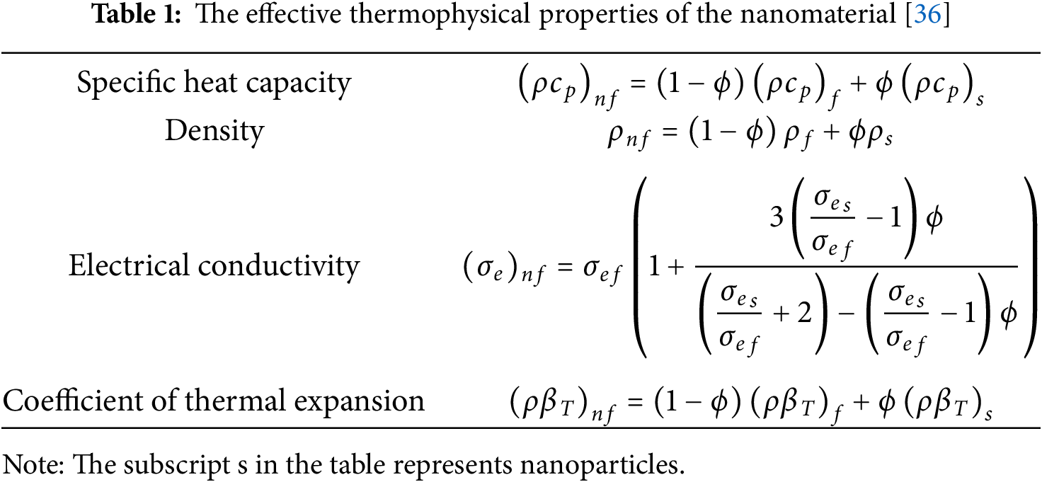
The surface-tension-induced boundary layer mixed convective flow of alumina-water nanomaterial is considered along with a significant buoyancy force. The buoyant force is significant because of the gravitational pull on the surface of the Earth. The working fluid considered in the study is alumina water as it possesses higher thermophysical properties, making it suitable for heat transfer applications. The alumina nanoparticles are suspended uniformly in thermal equilibrium and without slip. Fluid is incompressible and a laminar flow is considered. The nanomaterial is modeled using the homogeneous single-phase approach which includes the effective thermophysical properties of the nanomaterial. As seen in Fig. 1, the x-axis is along the fluid interface, and the y-axis is in the normal direction. A varying magnetic field is applied perpendicular to the interface and thermal radiative heat flux is considered in the system. There is no induced magnetic field as the magnetic Reynolds number is considered to be negligibly small. This results in a purely diffusive magnetism with an insignificant advection. Viscous dissipation and Joule heating effects are negligibly small. The vector form of the governing equations by using the conservation laws yield the following equations (see Chamkha et al. [5], and Golia et al. [29]):

∇⋅q=0,(2)

ρnf(∂q∂t+(q⋅∇)q)=−∇p+μnf∇2q−Γ{(ρβT)nf(T−T∞)}g+FL,(3)

(ρcp)nf(∂T∂t+(q⋅∇)T)=−∇(qr−knf∇T)−Q0(T−T∞).(4)

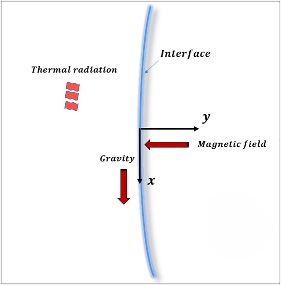
Figure 1: Physical model and geometry

In the above equations, the velocity vector for the two-dimensional flow is q=(u,v) in (x, y) direction, p is the pressure, T is the fluid temperature, t is time, T∞ is the ambient temperature, FL=J×B is the Lorentz force, J is the current density vector, B is the magnetic field vector, and Q0>0 is the heat sink coefficient. ∇ and ∇2 gradient and Laplacian operators. The gravity vector is aligned downward along with the interface. Also, as the normal component of gravity vector is assumed to be neglected, hence the curvature of the interface can be ignored. Moreover, the order-of-magnitude analysis also underpin this (see Napolitano et al. [30]). The Rosseland radiative heat flux is denoted by qr=−4σ∗3k∗∇T4, where, σ∗ (=5.67×10−8 W/m2K4) is the Stefan-Boltzmann constant and k∗ is the coefficient of mean absorption. The nanofluid thermophysical properties are μ (viscosity), ρ (density), cp (specific heat), βT (thermal expansion coefficient), and k (thermal conductivity). The subscripts nf and f represent the nanofluid and basefluid correspondingly.

Neglecting the displacement currents, the Maxwell field equations (electromagnetic) are as follows (see Sutton et al. [31]):

∇⋅B=0,∇×B=μ0J,∇×E=−∂B∂t,(5)

J=(σe)nf[E+q×B],(6)

where, (σe)nf is the electrical conductivity of the nanofluid, E is the electrical field vector, and μ0 is the magnetic permeability. But since there is no applied electric field, E=0. It is customary to assume that the magnetic field lines are fixed for the fluid. Moreover, Hall current and ion-slip currents are neglected.

Under the Boussinesq and Prandtl’s boundary layer approximations, the governing equations for the two-dimensional steady flow are as follows:

∂u∂x+∂v∂y=0,(7)

ρnf(u∂u∂x+v∂u∂y)=ρnfueduedx+μnf∂2u∂y2−(σe)nfB2(u−ue)−Γg(ρβT)nf(T−T∞),(8)

(ρcp)nf(u∂T∂x+v∂T∂y)=knf∂2T∂y2−∂qr∂y−Q0(T−T∞).(9)

The boundary conditions are given below:

Aty=0,v=v0,T=Ts=T∞+Axn+1,μnf∂u∂y=−∂σ∂x=−dσdT∂T∂x.Asy→∞,u→ue(x),T→T∞.(10)

where, ue denotes the external velocity, v0 is the suction/injection velocity and A is a constant. The third boundary condition at the interface (y=0) is due to the Marangoni effect which is not a bulk phenomenon and hence occurs at the boundary [32]. Here, the gradient of the stress tensor at the surface is equated to the surface tension gradient [33]. From the application point of view, it is imperative to study the heat transport characteristics associated with the flow problem. This can be quantified using the Nusselt number which is defined as follows:

Nux=−xkf(Ts−T∞)(knf∂T∂y−qr)y=0.(11)

In Eq. (8), the pressure gradient is reduced due to the presence of external flow, as shown below:

dpdx=−ρnfueduedx−(σe)nfB2ue.(12)

In various flow scenarios, the buoyant forces may assist or oppose the convective flow and hence, the dimensionless parameter Γ=±1 (for buoyancy forces that assist and oppose the flow) is used to distinguish these flow cases.

The optically dense nature of the water-based nanomaterial makes the Rosseland approximation suitable to model the radiative heat flux (see Rosseland [34]). Therefore, it is modeled as follows:

qr=−4σ∗3k∗∂T4∂y=−16σ∗T∞33k∗∂T∂y.(13)

The expression in Eq. (13) is obtained by approximating the Taylor series expansion of T4 about T∞ linearly. Therefore, Eq. (9) becomes:

(ρcp)nf(u∂T∂x+v∂T∂y)=(knf+16σ∗T∞33k∗)∂2T∂y2−Q0(T−T∞).(14)

2.2 Nanofluid Models

The single-phase nanofluid model is employed in conjunction with experimentally obtained relations to capture the properties of the 47 nm alumina-water nanomaterial. The nanomaterial viscosity is modeled using the Corcione model [35] which is an experimentally estimated relation as given below:

μnf=μf1−34.87(dpdf)−0.3ϕ1.03,(15)

where, dp=47 is the nanoparticle diameter, df=0.1(6WNπρf)13, W is the molecular weight of water, N denotes the Avogadro number, ϕ denotes the nanoparticle loading and ρf denotes the density of water at room temperature. The above model is valid for 25nm≤dp≤200nm, 0.01%≤ϕ≤7.1%, and in the temperature range 293–323K.

The thermal conductivity is also modelled using the Corcione model [35] which is given as follows:

knf=kf{1+4.4(Renf)0.4Pr0.66(TTfr)10(kpkf)0.03ϕ0.66},(16)

where, Renf=2ρfkBTπμf2dp—nanomaterial Reynolds number, kB—Boltzmann constant, μf—dynamic viscosity of water, Pr—Prandtl number of water, T—nanomaterial temperature, Tfr—freezing point of water, and kp denotes the thermal conductivities of alumina nanoparticle. This model is valid for 10nm≤dp≤150nm, 0.2%≤ϕ≤9% and 294K≤T≤324K. The remaining nanomaterial properties are computed using the conventional mixture theory (see Table 1).

2.3 Non-Dimensionalization

The following variables are used to arrive at non-dimensionality in the equations.

U=uUc,Ue(X)=ue(x)Uc,V=vδUc,V0=v0δUc,X=x−L0L,Y=yδL,T1=T−T∞ΔT,T1S=Ts(x)−T∞ΔT.(17)

In the above equations, Uc is the reference velocity defined as νfLδ2, Re is the Reynolds number defined as σTΔTLνfμf, δ is the scale factor defined as Re−13, and L is the scale length. Also, the origin of the x-axis is at L0 and ΔT represents the incremental temperature in the system.

Using (17) in Eqs. (7)–(10), one can get:

∂U∂X+∂V∂Y=0,(18)

ρnfρf(U∂U∂X+V∂U∂Y)=ρnfρfUedUedX+μnfμf∂2U∂Y2−(σenfσef)M∗(U−Ue)−Γ(ρβT)nf(ρβT)fλT1,(19)

(ρcp)nf(ρcp)f(U∂T1∂X+V∂T1∂Y)=1Pr(knfkf+R)∂2T1∂Y2−Q∗T1,(20)

AtY=0:V=V0,T1=T1S(X),μnfμf∂U∂Y=∂T1∂X.(21)

AsY→∞:U→Ue(X),T1→0.(22)

where,

Pr=μfcpfkf(Prandtl number),

λ=g(βT)fΔTLUc2(thermal buoyancy parameter),

Q∗=Q0L(ρcp)fUc(heat sink factor),

M∗=(σe)fLB2ρfUc(magnetic factor),

R=16σ∗T∞33k∗kf(radiation parameter).

Self-similar solutions are computed by using the similarity transformations given below (see Golia et al. [29]):

U=U0X3f′(ζ),V=−U0l0X[2f(ζ)+ζf′(ζ)],T1=−t0X5θ(ζ),V0=−U0l0XS,Ue(X)=U0X3,B=B0Xl0,Q0=QX2l02ζ=XYl0.(23)

where, f′,θ,S are respectively the dimensionless velocity, temperature, and suction/injection parameter and prime denotes the differentiation with respect to the similarity variable. U0,l0,t0 are constant non-dimensional scale factors such that (see Golia et al. [29]):

U0l02=12,t0l02U0=1,t0l0U0=15.(24)

The set of ordinary differential equations is obtained as follows:

μnfμff′′′+32ρnfρf(1−(f′)2)+ρnfρfff′′+Γ(ρβT)nf(ρβT)fλθ−(σenfσef)M(f′−1)=0,(25)

1Pr(knfkf+R)θ′′−(ρcp)nf(ρcp)f(52f′θ−θ′f)−Qθ=0,(26)

with

f(0)=S,(μnfμf)f′′(0)=−1,θ(0)=1,

f′(∞)→1,θ(∞)→0.(27)

The non-dimensional scaled form of Eq. (11) is obtained as follows:

Nux=−(knfkf+R)θ′(0).(28)

2.4 Entropy Generation

It is extremely important to make the heat transfer thermodynamically stable. Heat transfer produces thermodynamic irreversibility or entropy generation. Therefore, it is worth studying entropy generation. Lower entropy leads to lower energy loss. The viscous and Joule heating effects have been neglected in the energy equation to study heat transfer. But an order of magnitude analysis indicates that they are important in studying the entropy generation. Therefore, the entropy generation can be modelled as follows (see Bejan [37]):

SG=kfT∞2(knfkf+16σ∗T∞33k∗kf)(∇T)2+μnfT∞(∇u)2+(σe)nfB2T∞u2.(29)

Under the assumptions of the present problem:

SG=kfT∞2(knfkf+16σ∗T∞33k∗kf)(∂T∂y)2+μnfT∞(∂u∂y)2+(σe)nfB2T∞u2,(30)

The terms of SG respectively represent the irreversibility due to the heat transfer, viscous dissipation, thermal radiation, and Joule heating. After non-dimensionalization and suitable scaling, the dimensionless form is obtained as follows:

NG=(knfkf+R)(θ′)2+μnfμfBr(f′′)2+(σe)nf(σe)fMBr(f′)2,(31)

where, NG=SGT∞2δ2L2l02kf(ΔT)2t02X12 and Br=μfUc2T∞U02kf(ΔT)2t02X4.

The ratio of heat transfer irreversibility to the total irreversibility is called the Bejan number (Be) which is given as Be=Entropy rate due to heat transferTotal entropy.

Be=(knfkf+R)(θ')2(knfkf+R)(θ')2+μnfμfBr(f'')2+(σe)nf(σe)fMBr(f')2(32)

The value of Be ranges between 0 and 1, where 0 signifies the case where there is no generation of entropy due to heat transport and 1 signifies the case where the generation of entropy is only due to heat transport.

2.5 Numerical Solution

The system of equations Eqs. (25)–(27) is converted to a set of first-ordered differential equations using f=y1,f′=y2,f′′=y3,θ=y4, and θ′=y5 to get the equations below:

y1′=y2,(33)

y2′=y3,(34)

y3′={(ρnfρf)[(32)((y2)2−1)−y1y3]−Γ(ρβT)nf(ρβT)fλy4−(σenfσef)M(1−y2)}(μfμnf),(35)

y4′=y5,(36)

y5′=Pr{((ρcp)nf(ρcp)f)[(52)y2y4−y1y5]+Qy4}[(knfkf)+R].(37)

This obtained system is then solved using Ralston’s fourth-order method [38]. This method is a self-starting numerical method with minimum truncation error which makes it advantageous to record accurate results. The method is a modified Runge-Kutta method which involves the following set of equations in the algorithm [38]:

yn+1−yn=0.17476028k1−0.55148066k2+1.2055356k3+0.17118478k4,(38)

where,

k1=hf(xn,yn),(39)

k2=hf(xn+0.4h,yn+0.4k1),(40)

k3=hf(xn+0.45573725h,yn+0.29697761k1+0.15875964k2),(41)

k4=hf(xn+h,yn+0.2181004k1−3.05096516k2+3.83286476k3).(42)

In the computations, infinity is rescaled to 5 as increasing this value does not have a significant change in the results. The domain is divided into 100 subintervals in the computational frame. The missing boundary conditions (f′(0) and θ′(0)) are estimated with the help of suitable guess values. The accuracy of the results is ensured by utilizing a relative error tolerance of 10−6 in the computations.

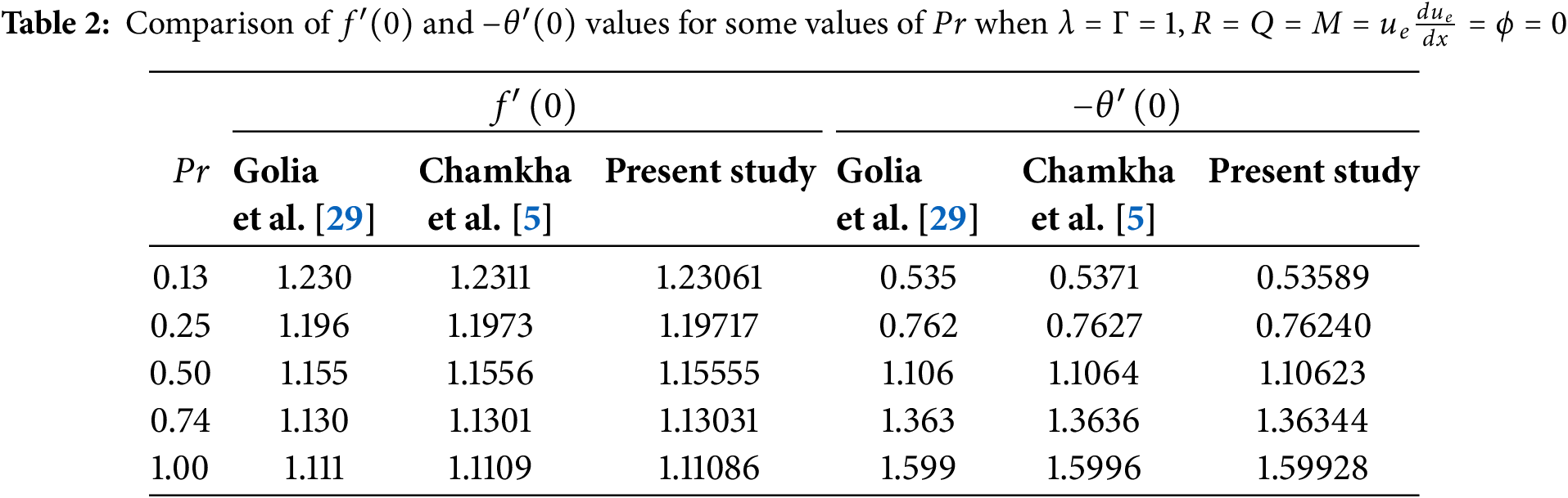
The numerical accuracy of the method is evaluated by a restrictive correspondence with the literature. The Marangoni-buoyant boundary layer case when the buoyancy is opposing is considered in the absence of radiative, magnetic, and heat sink effects. Golia et al. [29] employed the quasi-linearization method to arrive at numerical solutions whereas Chamkha et al. [5] used an implicit finite difference method. As seen in Table 2, the numerical values are accurate and hence uphold the accuracy of the numerical methodology employed in the present study.

3  Optimization Procedure

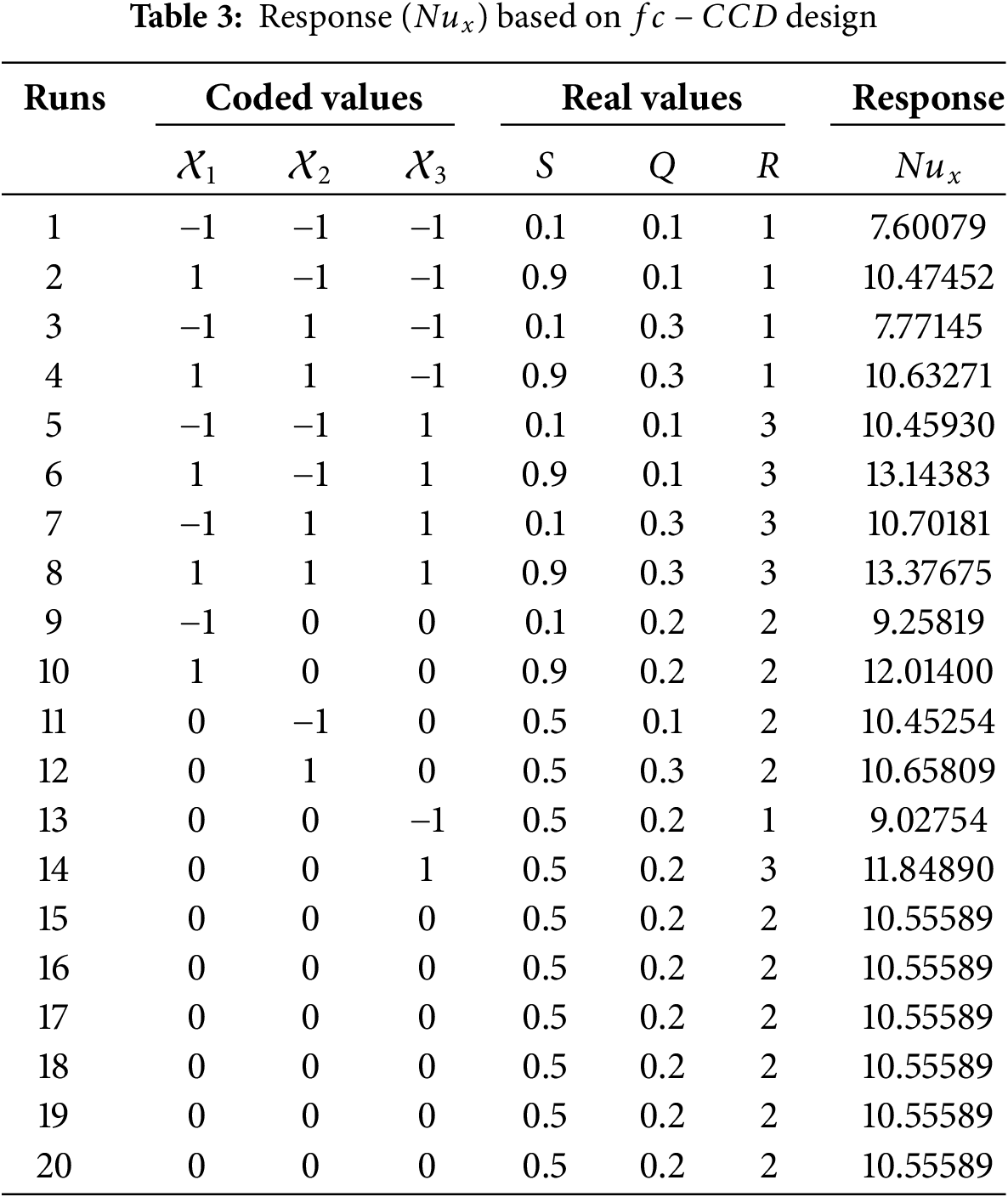
RSM is a robust tool based on Design of Experiments (DoE) which involves mathematical and statistical aspects. RSM is beneficial especially in situations to optimize a process and to study the interactive effects. Here, the heat transfer rate (quantified by Nux) is used as the response variable and injection (0.1≤S≤0.9), internal heat sink (0.1≤Q≤0.3), and thermal radiation (1≤R≤3) are chosen as the factor variables. The factor variables are coded as 𝒳1,𝒳2 and 𝒳3, respectively. Due to the advantage of including extreme points in the design, the face-centered (fc) Central Composite Design is employed in the computations. The count of runs in the design is calculated based on the formula 2q+2q+p, where q and p represent the number of parameters and faces respectively. Table 3 gives the numerical experimental design. This methodology yields an empirical relation which is of quadratic order as given below:

𝒴=r0+∑i=13ri𝒳i+∑∑i≤j=13rij𝒳i𝒳j(fori,j=1,2,3),(43)

where, r0 is an intercept, ri and rij denote the respective regression coefficients, and 𝒴 and 𝒳 denote the response and independent variables, respectively.

Optimization of the response variable is done based on the desirability value approach. The range of the desirability value is 0 to 1. For the maximization objective, the desirability value for each run is calculated as follows:

di=0,𝒴i≤𝒴L,di=𝒴i−𝒴L𝒴H−𝒴L,𝒴L≤𝒴i≤𝒴H,di=1,𝒴i≥𝒴H,(44)

where, 𝒴H and 𝒴L denote the highest and lowest response respectively. The total desirability (D) is the geometric mean of the individual desirabilities which is maximized to obtain the optimum (maximized) condition. The total desirability is estimated as follows:

D=(∏i=1ndi)1n.

4  Results and Discussion

The findings of the parametric and statistical computations are presented in this section and discussed with physical interpretations. Furthermore, the sensitivity of the heat transport is analyzed.

4.1 Discussion of Parametric Results

In this subsection, the impact of a single pertinent parameter on the flow and thermal profiles is analyzed by fixing the other parameters. The profiles for three types of boundaries (i.e., suction, impermeability, and injection) are compared. The Prandtl number which is a fluid property is fixed at 6.0674 (calculated for water at 300 K). Moreover, the domain is rescaled to 0 to 3 as there is no appreciable change in the numerical values by increasing the domain further.

A larger radiative heat flux leads to a higher velocity of the nanomaterial as one can observe from Fig. 2. This is because of the higher energy supplemented to the system by the radiation. Also, the flow profile in the irradiative situation (R=0) possesses the lowest flow profile. Also, the suction flow has a higher velocity when compared to impermeable and injection flow cases. Furthermore, the effect of the applied magnetic field is explored in Fig. 3. The Lorentz force produced due to magnetism in the nanomaterial tends to oppose the flow and therefore the velocity decreases. The flow in the absence of magnetism is depicted by the curves when M=0.

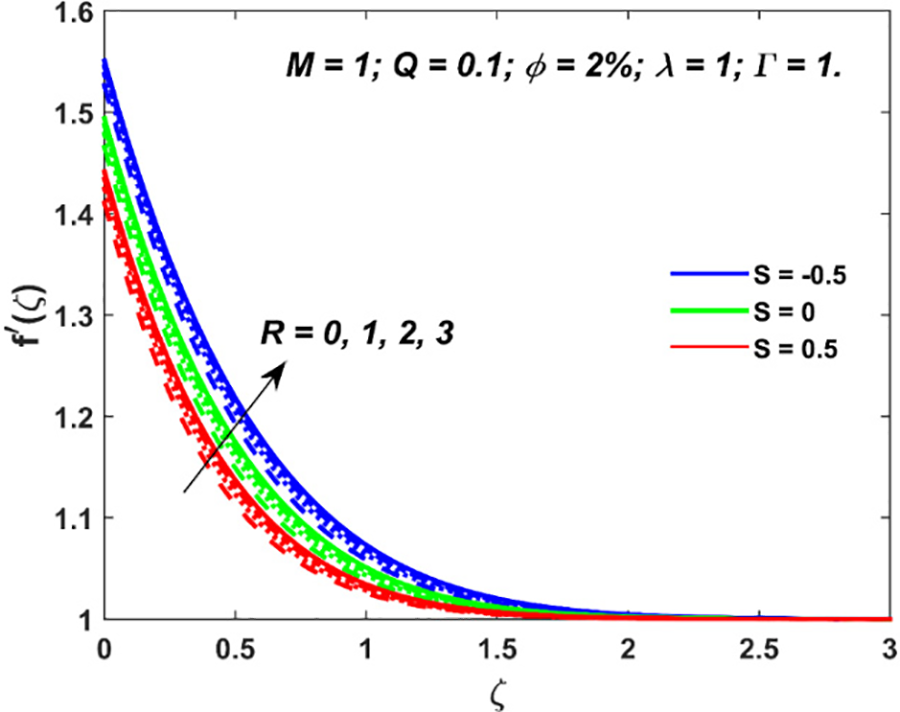
Figure 2: Variation in nanofluid velocity due to R

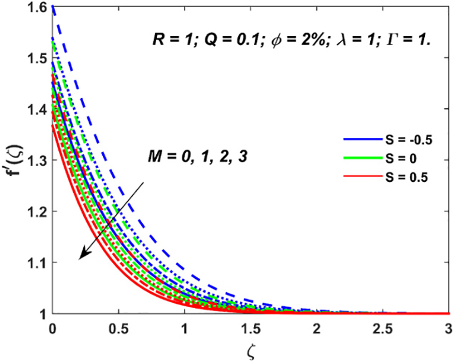
Figure 3: Variation in nanofluid velocity due to M

The increment in λ leads to higher buoyant force and this has an opposing effect on the fluid thermal profile as can be seen in Fig. 4. The additional energy provided by the radiative heat flux has a significantly increasing impact on the thermal profile and hence the regulation of the radiative heat provided to the nanomaterial can be used to augment the temperature profile (see Fig. 5). In Fig. 6, the temperature rise due to the applied magnetic field is observed. This trend is seen due to the Lorentz force formed by the magnetic force. The heat sink absorbs energy from the fluid and hence the nanomaterial temperature decreases (see Fig. 7). Moreover, it can be observed that the flow with suction possesses a higher thermal profile when compared to impermeable and injection cases.

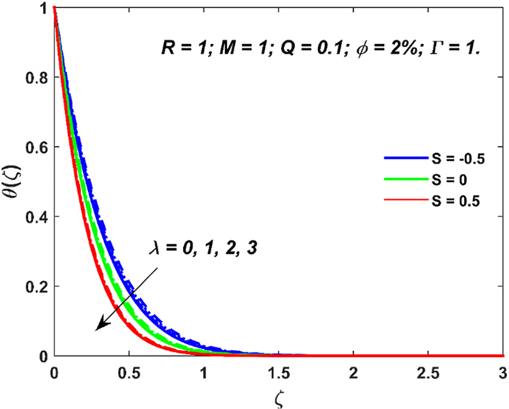
Figure 4: Variation in nanofluid temperature due to λ

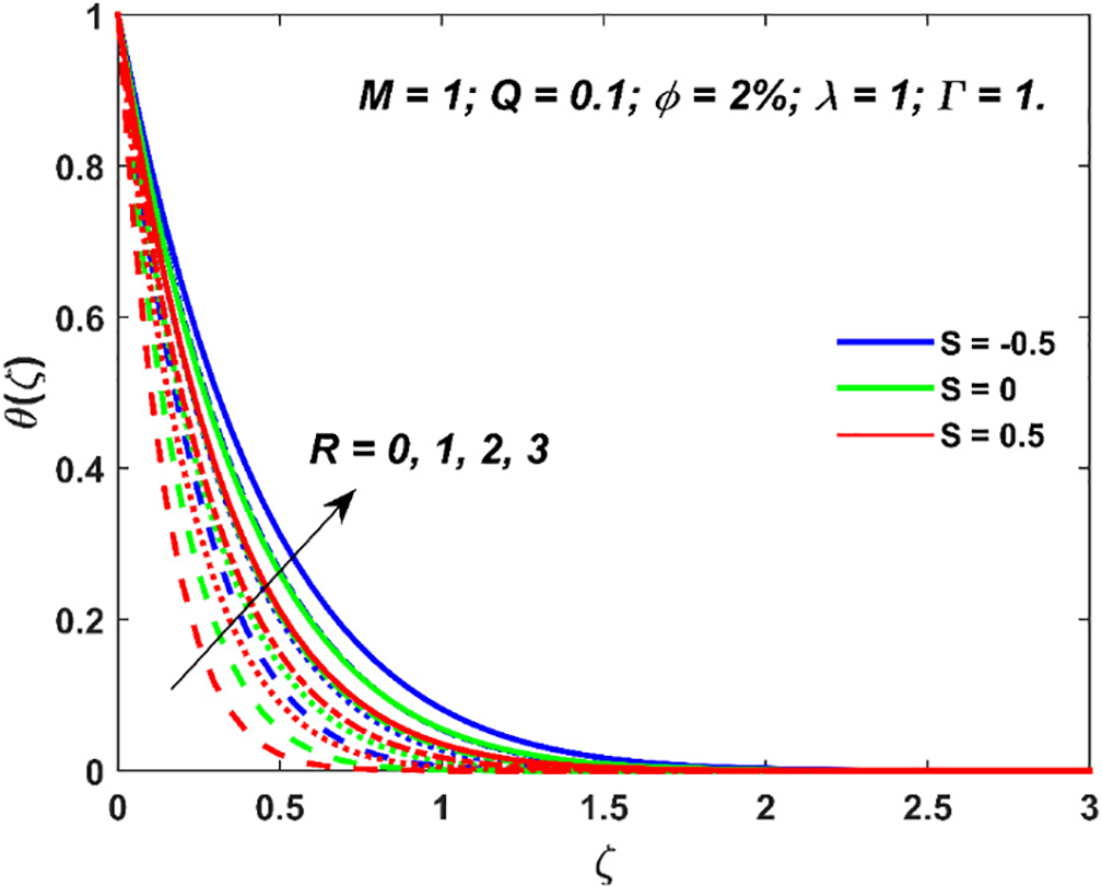
Figure 5: Variation in nanofluid temperature due to R

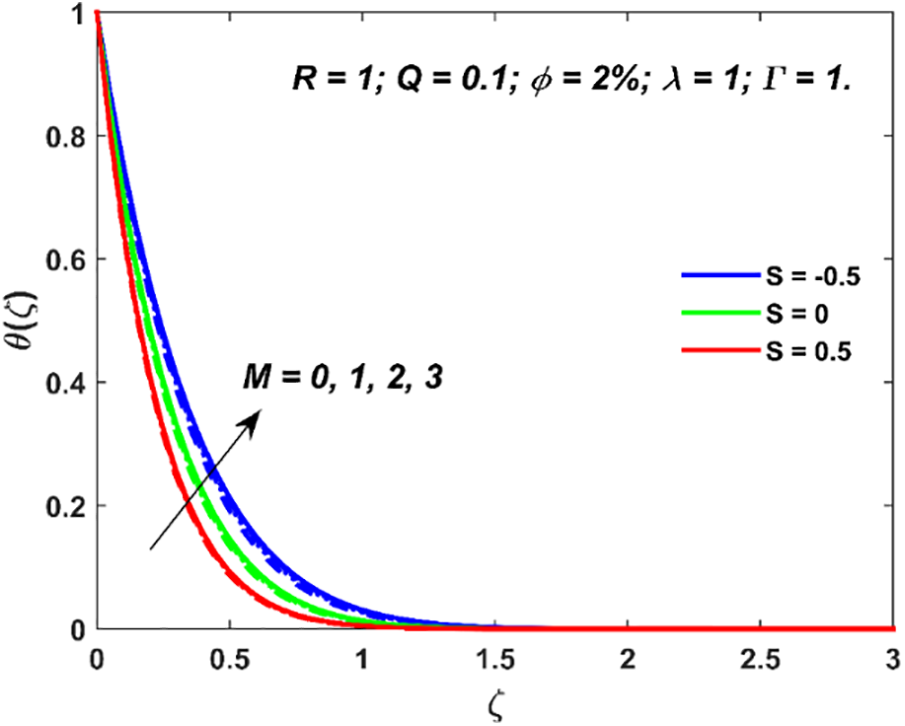
Figure 6: Variation in nanofluid temperature due to M

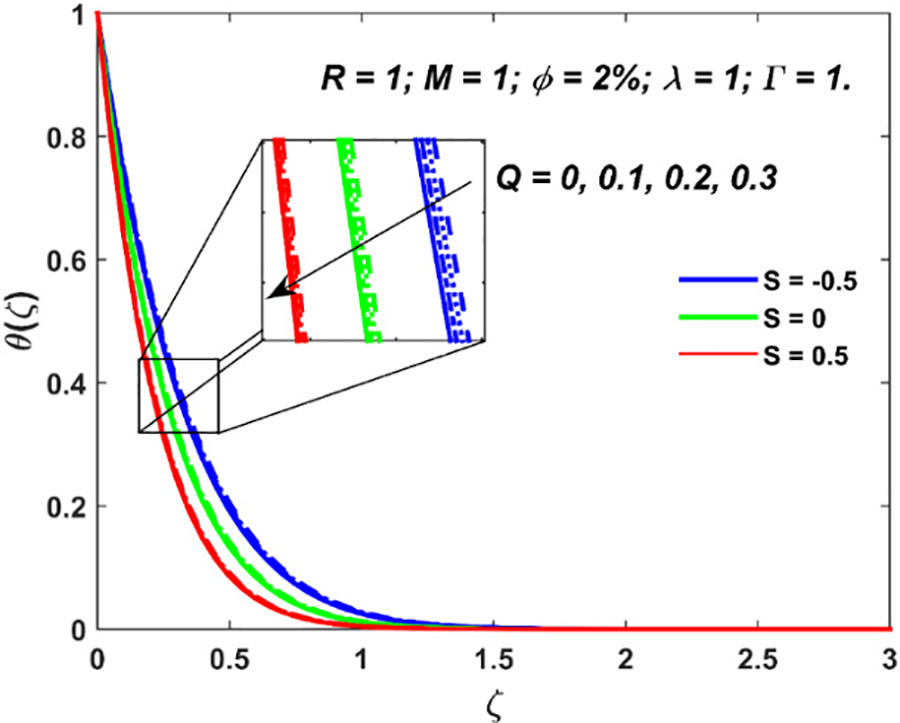
Figure 7: Variation in nanofluid temperature due to Q

The characteristics of entropy generation and Bejan number are visualized in Figs. 8–13. The entropy generation decays with an increment in Br as seen in Fig. 8. Physically this is because the increased heat generated in the fluid increases the disorderliness and therefore the entropy generation augments. Also, the Bejan number is decreased (see Fig. 9) which signifies that the viscous heating and Joule heating effects become more dominant with the increment of Br. Figs. 10 and 11 illustrate the effect of M on NG and Be, respectively. A rise in NG and a decrease in Be is observed which is because of the enhancement in both viscous friction forces and magnetic resistance instigated by the Lorentz forces in the fluid system. The entropy generation and Be are magnified by the increment in R as one can see from Figs. 12 and 13. The applied thermal radiation provides additional energy that increases the disorderliness and also supplements the heat transport. Thus, the entropy generation is incremented and the heat transfer irreversibility becomes more dominant over other irreversibilities considered.

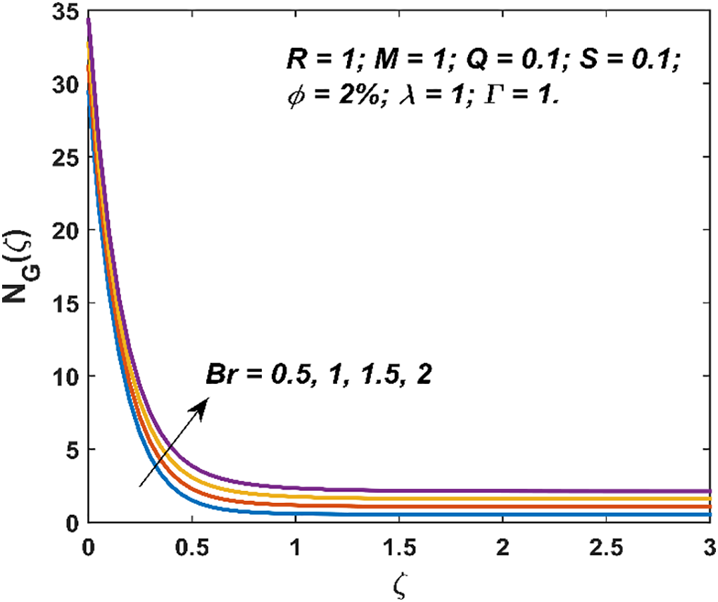
Figure 8: Variation in entropy generation due to Br

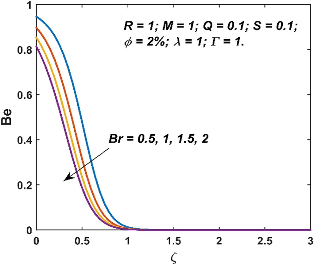
Figure 9: Variation in Bejan number due to Br

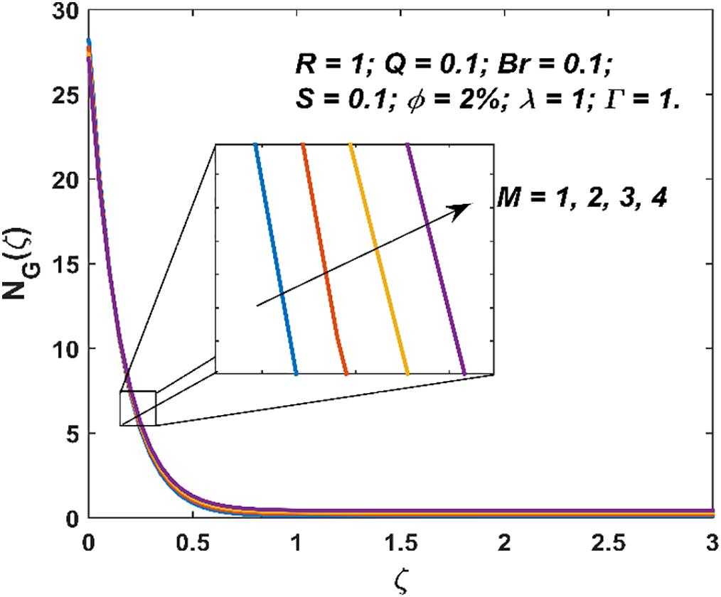
Figure 10: Variation in entropy generation due to M

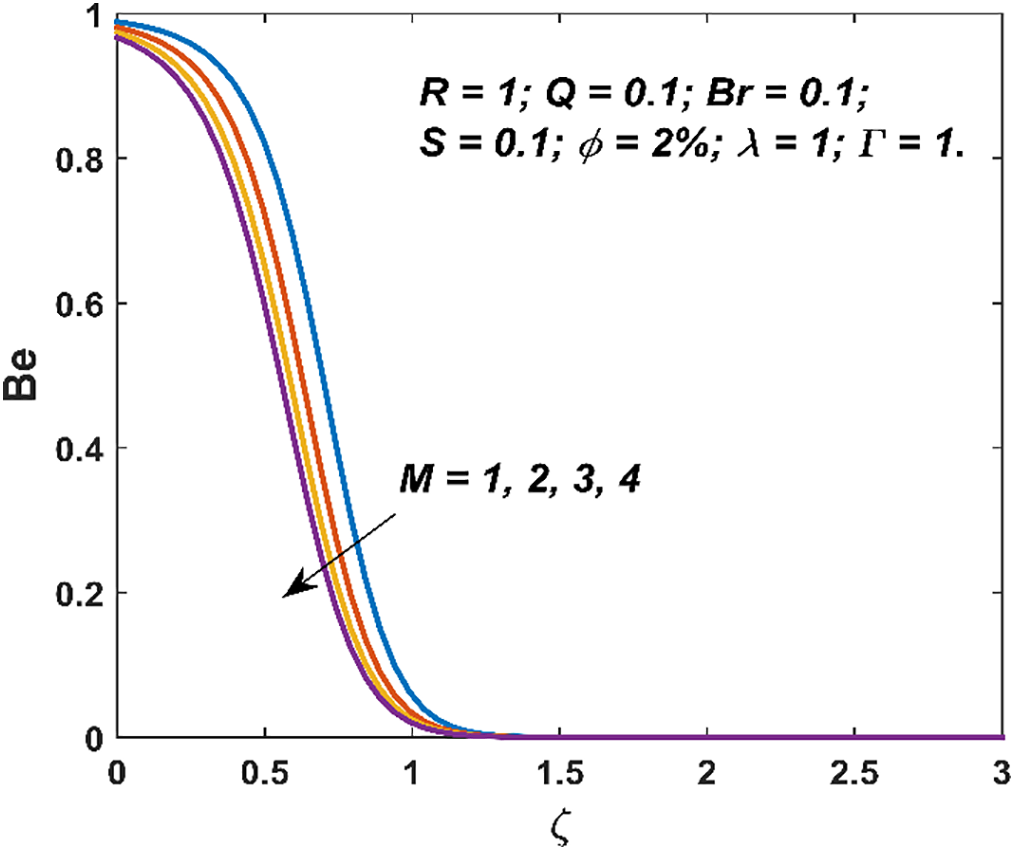
Figure 11: Variation in Bejan number due to M

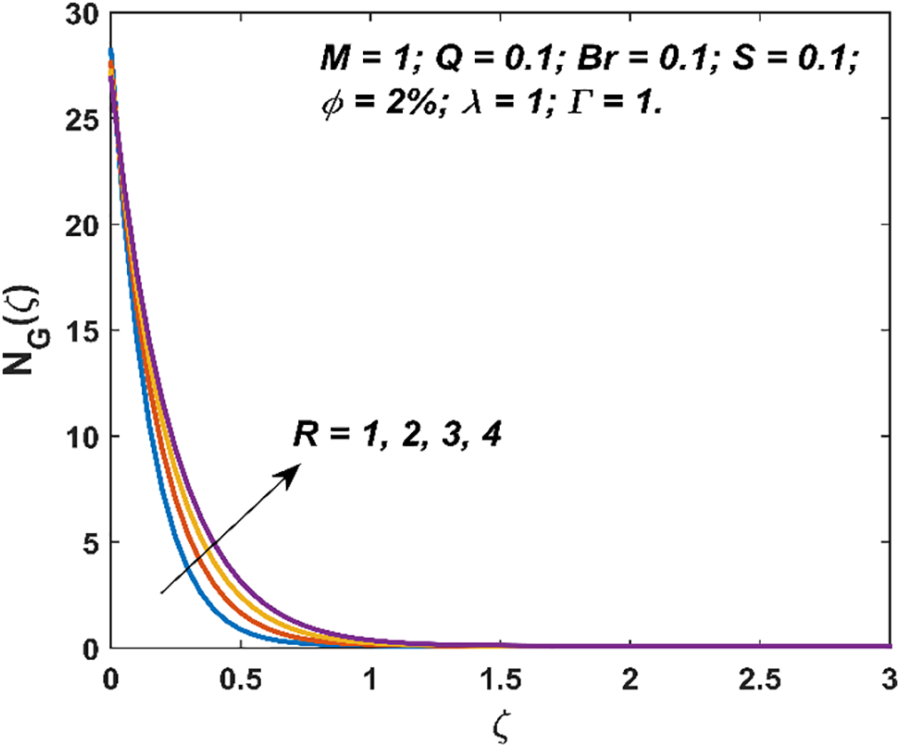
Figure 12: Variation in entropy generation due to R

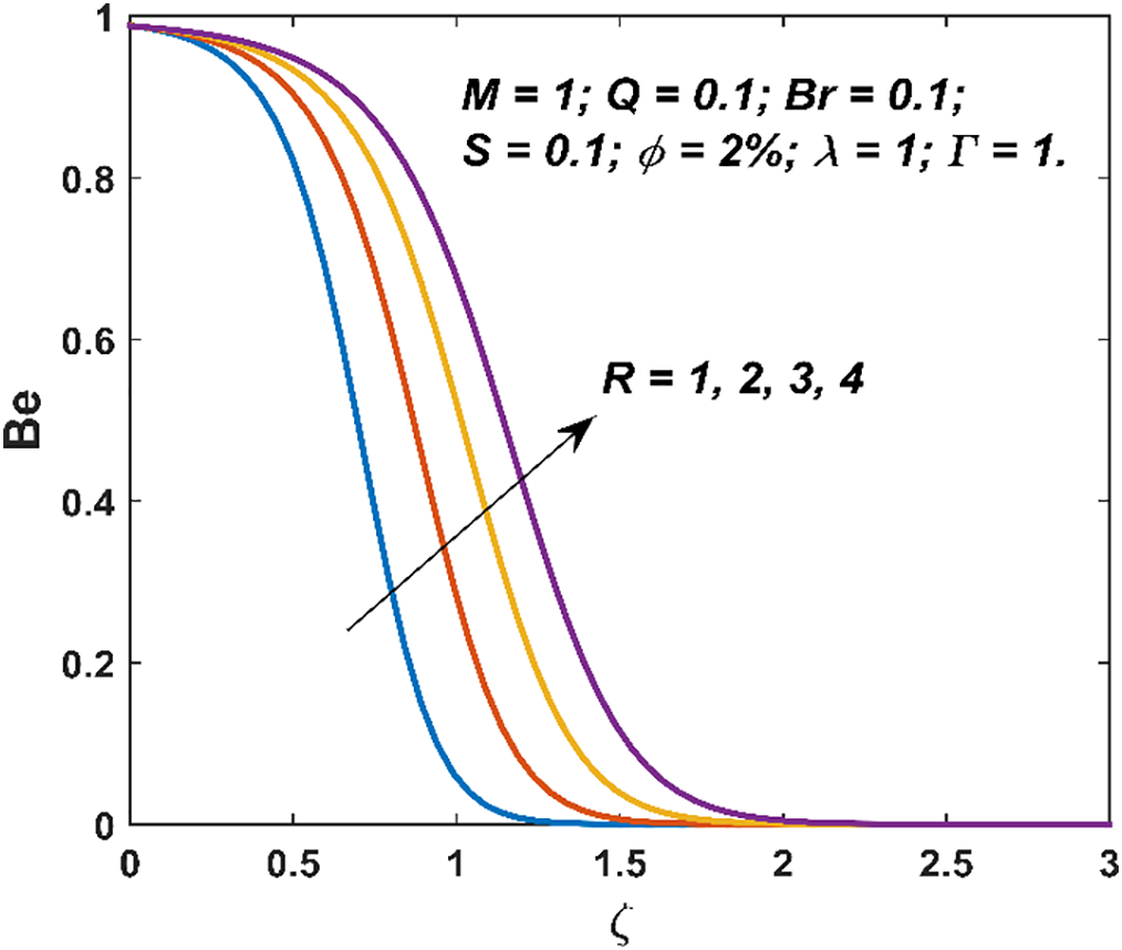
Figure 13: Variation in Bejan number due to R

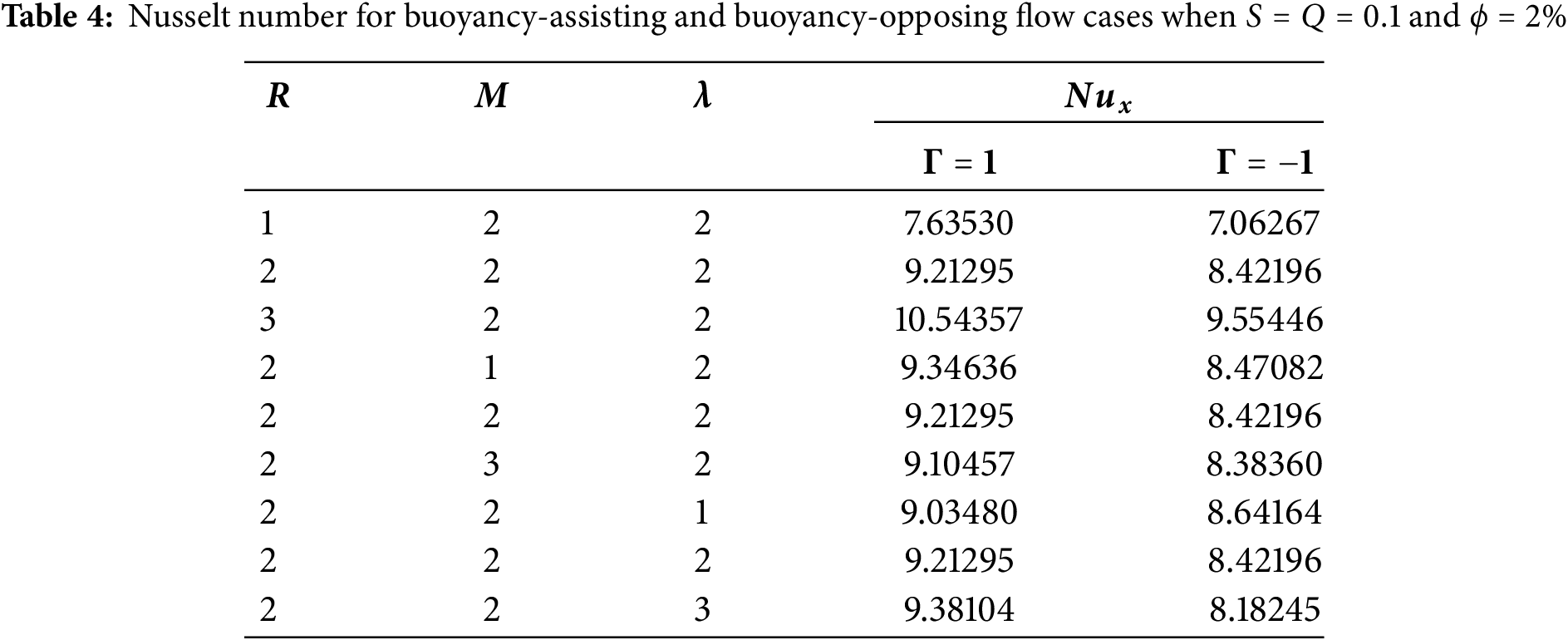
In Table 4, the heat transport at the interface for buoyancy assisting and buoyancy opposing flow scenarios are tabulated. The Nusselt number is higher when Γ=1 when compared with the Γ=−1 case. Moreover, it can be observed that increment in R increases the heat transport at the interface due to larger energy in the fluid system. On the other hand, a rise in M decreases Nux which is caused by the Lorentz force developed in the fluid system. Also, λ has an opposing effect on Nux in both flow scenarios which is caused by an enhancement in buoyant forces. This result is in agreement with that reported by Chamkha et al. [5].

4.2 RSM Analysis Results

The output of the analysis of variance (ANOVA) table are given in Table 5. The significance of the RSM model terms is benchmarked via the p-value at 95% level of significance. The significance is assured if p-value < 0.05. The interaction term of Q and S along with the quadratic term of Q are insignificant and are therefore removed from the RSM model. Moreover, the coefficient of determination (which indicates the variation in the dependent variable that could be explained by the chosen independent variables) ℛ2 is 99.99% which upholds the model accuracy. The fitted quadratic model comprising the significant uncoded model terms (linear, interaction, and quadratic) is given below:

Nux=3.2046S+0.668Q+1.8917R+0.5065S2−0.11683R2−0.0689SQ−0.11735SR+0.1832QR+5.4270.(45)

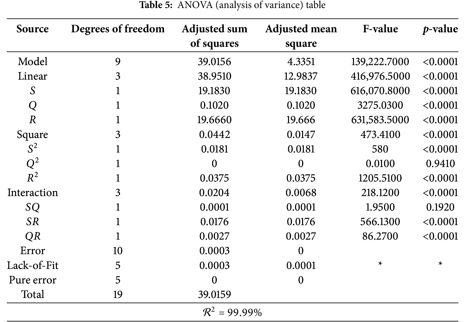
This fitted model can be used to accurately estimate the heat transport in the chosen ranges of the parameters due to high ℛ2. The accuracy of the RSM model is also assured by the residual plots (see Fig. 14) which indicate the normal nature of the residuals and also show that the maximum error in each run is less than 1%.

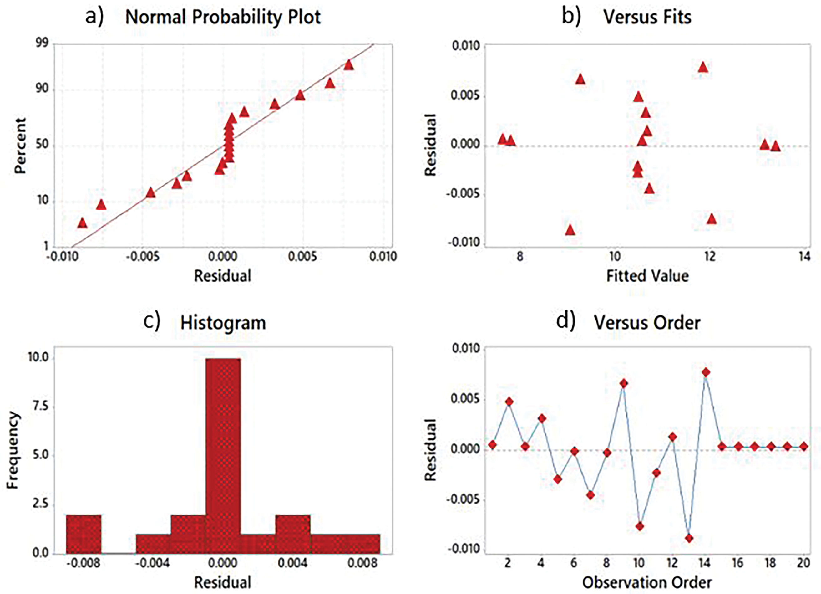
Figure 14: Residual plots. (a) ‘Normal Probability plot’, (b) ‘Versus fits’, (c) ‘Histogram’, (d) ‘Versus Order’

In Fig. 15, the interaction of two parameters is analyzed by fixing the third one at the medium level. Both Q and S lead to higher heat transport but it is observed that the increment in Q has a low impact on Nux (see Fig. 15a). The thermal radiation aspect increases the heat transport with a much higher intensity than Q as one can see from Fig. 15b. Fig. 15c provides a comparison of the relative incremental effect of R and S on the heat transfer.

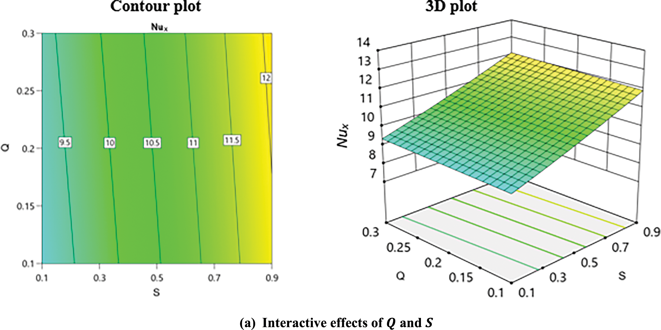
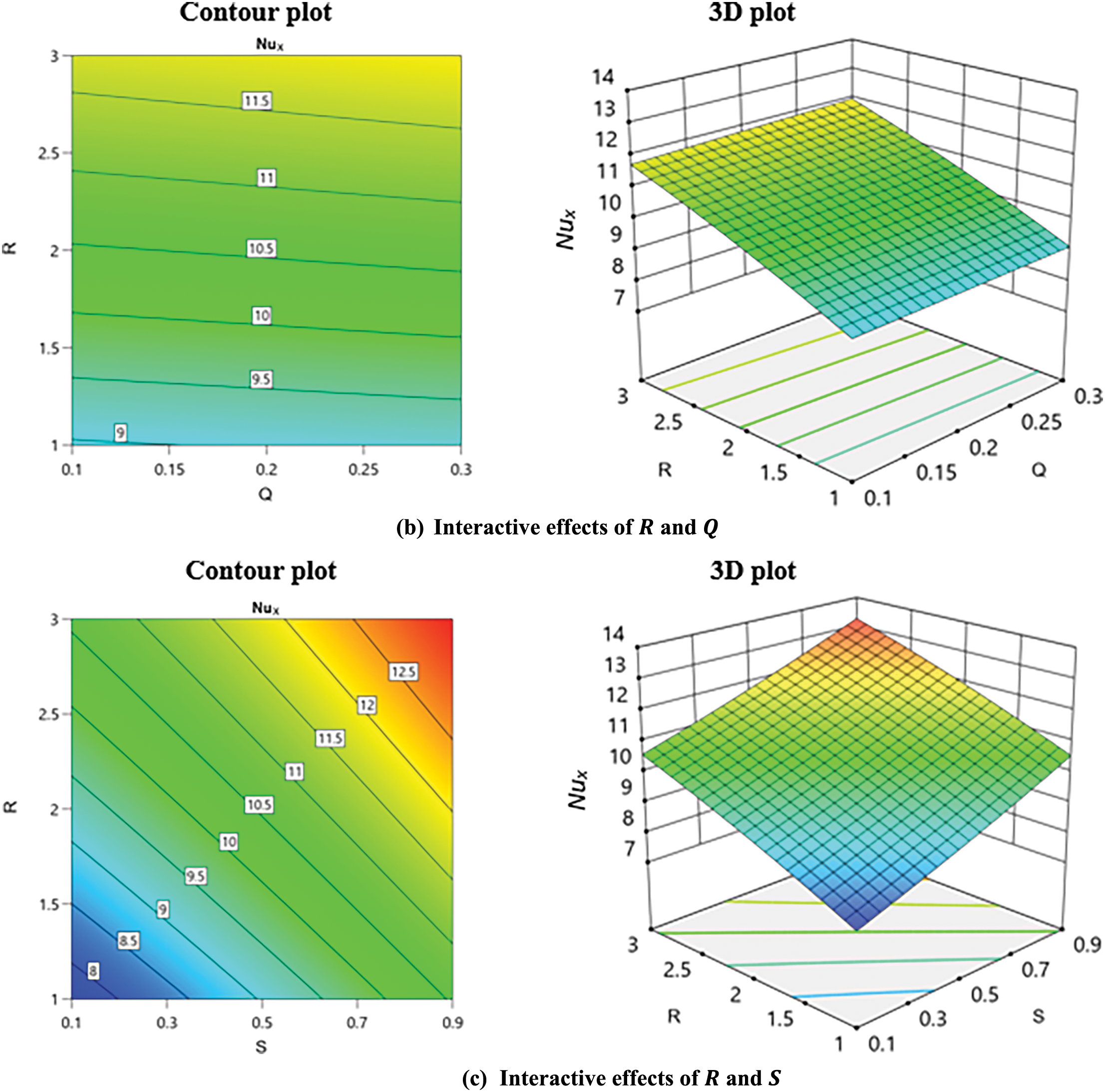
Figure 15: 3-D and contour plots for heat transport at the interface. (a) Interactive effects of Q and S. (b) Interactive effects of R and Q. (C) Interactive effects of R and S

Optimized Nux=13.377 is obtained at the high levels of S,Q, and R with desirability, d=1. The 95% Confidence interval for the optimized heat transport is calculated to be [13.3659, 13.3881].

4.3 Sensitivity Analysis

Analyzing the sensitivity of the heat transfer rate at the interface towards S,Q, and R is crucial in situations where the heat transport needs to be controlled or regulated. The change in the Nusselt number due to an incremental change in the factor variables is measured by the sensitivity value. A positive sensitivity signifies that the variables are positively correlated and the magnitude can be used for relative comparison. The empirical model utilizing the coded factor variables is given below:

Nux=1.38503𝒳1+0.10098𝒳2+1.40236𝒳3+0.08104𝒳12−0.11683𝒳32−0.04694𝒳1𝒳3+0.01832𝒳2𝒳3+10.5556.(46)

Partial derivatives of Eq. (46) denote sensitivity functions for 𝒳1,𝒳2 and 𝒳3, respectively, which are as follows:

∂Nux∂𝒳1=1.38503+0.16208𝒳1−0.04694𝒳3,(47)

∂Nux∂𝒳2=0.10098+0.01832𝒳3,(48)

∂Nux∂𝒳3=1.40236−0.04694𝒳1+0.01832𝒳2−0.23366𝒳3.(49)

Table 6 shows the sensitivity values of Nux at all levels. It is found that the sensitivity towards S,Q, and R is positive indicating that a change in these parameters leads to an increment in the heat transfer. The sensitivity towards the heat sink is relatively lesser.

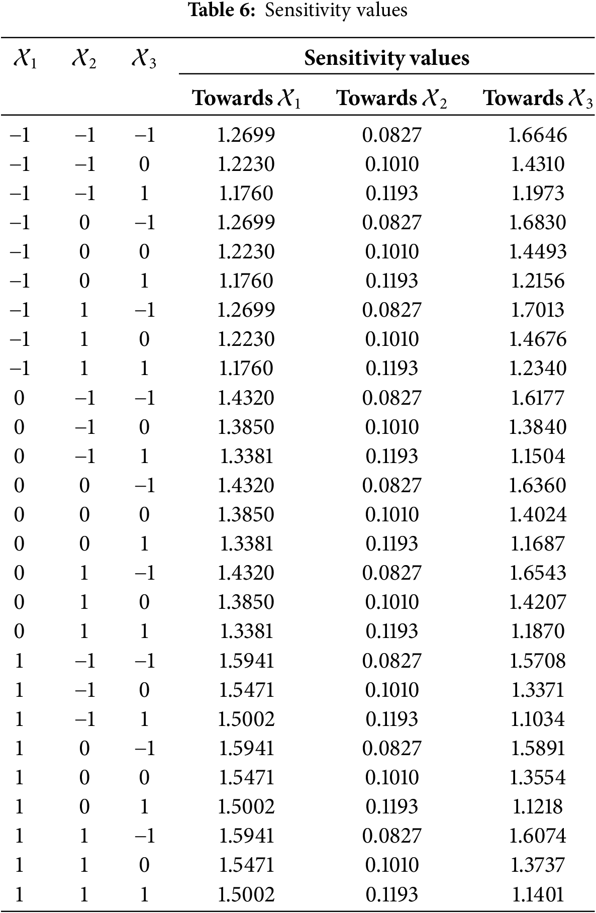
The highest sensitivity is observed at the low levels of S and R and high level of Q with a sensitivity magnitude of 1.7013. On the other hand, the lowest is observed when the parameters are at low levels. Further, the changes in the sensitivity values because of changes in the factor levels can be inferred from Table 6. This is useful for designers to decide which controlling constraint should be regulated to enhance higher heat transport.

5  Conclusions

The heat transfer rate in mixed thermal Marangoni convective flow of alumina-water nanoliquid in the presence of suction/injection and significant buoyant forces is optimized in this study. Additionally, radiative heat flux, magnetism, and an internal heat sink are considered in the model. The fourth order is Ralston’s method is used to find numerical solutions. This prototype developed to analyze the fluid flow and thermodynamic behavior with heat transfer optimization has led to the following major conclusions:

•   The flow profiles and the thermal fields are superior in the presence of suction instead of impermeable and injection flow scenarios.

•   The buoyant force has a prominent opposing effect on the temperature profile.

•   The entropy generation increases with more thermal radiation. This also leads to a higher Bejan number, indicating that heat transfer irreversibility is predominant.

•   The applied magnetism forms Lorentz forces in the fluid system which increment the disorderliness and hence generate more entropy.

•   The highest sensitivity of 1.7013 for the Nusselt number is observed at the low levels of injection and thermal radiation when the heat sink is at the high level.

•   The optimized heat transport (Nux=13.377) is recorded at the high levels of thermal radiation, injection, and heat sink.

•   The 95% Confidence interval for the optimized heat transport is calculated to be [13.3659, 13.3881].

•   The numerical results obtained via Ralston’s method were in good corroboration with the results of the limiting cases reported in the literature.

The model developed in this manuscript is a prototype for semiconductor crystal heat transfer, growth of silicon wafers, and coating processes [39].

Acknowledgment: The authors thank the learned reviewers and Editor for their constructive comments. The second author, Mahanthesh Basavarajappa, conducted this research during his tenure as a faculty member at Christ University. He sincerely thanks Christ University for the support.

Funding Statement: The authors received no specific funding for this study.

Author Contributions: The authors confirm contribution to the paper as follows: study conception and design: Joby Mackolil, Mahanthesh Basavarajappa; analysis and interpretation of results: Joby Mackolil, Mahanthesh Basavarajappa, Giulio Lorenzini; draft manuscript preparation: Joby Mackolil, Mahanthesh Basavarajappa; editing and supervision of the manuscript: Giulio Lorenzini. All authors reviewed the results and approved the final version of the manuscript.

Availability of Data and Materials: The data that support the finding are available from the corresponding author upon reasonable request.

Ethics Approval: Not applicable.

Conflicts of Interest: The authors declare no conflicts of interest to report regarding the present study.

References

1. Bergman TL. Numerical simulation of double-diffusive Marangoni convection. Phys Fluids. 1986;29(7):2103–8. doi:10.1063/1.865597. [Google Scholar] [CrossRef]

2. Laknath R, Mendis A, Sekimoto A, Okano Y, Minakuchi H, Dost S. A numerical study on the exact onset of flow instabilities in thermo-solutal marangoni convection driven by opposing forces in a half-zone liquid bridge under zero gravity. J Chem Eng Japan. 2021;54(8):424–30. doi:10.1252/jcej.21we041. [Google Scholar] [PubMed] [CrossRef]

3. Rosenblat S, Davis SH, Homsy GM. Nonlinear Marangoni convection in bounded layers. Part 1. Circular cylindrical containers. J Fluid Mech. 1982;120:91–122. doi:10.1017/S0022112082002687. [Google Scholar] [CrossRef]

4. Sen AK, Davis SH. Steady thermocapillary flows in two-dimensional slots. J Fluid Mech. 1982;121:163–86. doi:10.1017/S0022112082001840. [Google Scholar] [CrossRef]

5. Chamkha AJ, Pop I, Takhar HS. Marangoni mixed convection boundary layer flow. Meccanica. 2006;41(2):219–32. doi:10.1007/s11012-005-3352-y. [Google Scholar] [CrossRef]

6. Khan MI, Qayyum S, Chu YM, Khan NB, Kadry S. Transportation of Marangoni convection and irregular heat source in entropy optimized dissipative flow. Int Commun Heat Mass Transf. 2021;120:105031. doi:10.1016/j.icheatmasstransfer.2020.105031. [Google Scholar] [CrossRef]

7. Mackolil J, Mahanthesh B. Optimization of heat transfer in the thermal Marangoni convective flow of a hybrid nanomaterial with sensitivity analysis. Appl Mathem Mech-Eng Edit. 2021;42(11):1663–74. doi:10.1007/s10483-021-2784-6. [Google Scholar] [CrossRef]

8. Jiang Y, Dai C, Zhou X. Effect of interfacial heat transfer on hydrothermal wave propagation of nanofluid thermocapillary convection in rectangular cavity. Microgravity Sci Technol. 2024;36(43):1–17. doi:10.1007/s12217-024-10129-5. [Google Scholar] [CrossRef]

9. Abbas SZ, Khan MI, Kadry S, Khan WA, Israr-Ur-Rehman M, Waqas M. Fully developed entropy optimized second order velocity slip MHD nanofluid flow with activation energy. Comput Methods Programs Biomed. 2020;190:105362. doi:10.1016/j.cmpb.2020.105362. [Google Scholar] [PubMed] [CrossRef]

10. Jawad M, Saeed A, Kumam P, Shah Z, Khan A. Analysis of boundary layer MHD Darcy-Forchheimer radiative nanofluid flow with Soret and Dufour effects by means of Marangoni convection. Case Stud Therm Eng. 2021;23(2):100792. doi:10.1016/j.csite.2020.100792. [Google Scholar] [CrossRef]

11. Sneha KN, Bognar G, Mahabaleshwar US, Singh DK, Singh OP. Magnetohydrodynamics effect of Marangoni nano boundary layer flow and heat transfer with CNT and radiation. J Magn Magn Mater. 2023;575:170721. doi:10.1016/j.jmmm.2023.170721. [Google Scholar] [CrossRef]

12. Khan D, Kumam P, Khan I, Sitthithakerngkiet K, Khan A, Ali G. Unsteady rotating MHD flow of a second-grade hybrid nanofluid in a porous medium: laplace and Sumudu transforms. Heat Transfer. 2022;51(8):8065–83. doi:10.1002/htj.22681. [Google Scholar] [CrossRef]

13. Khan D, Ali G, Kumam P, Sitthithakerngkiet K, Jarad F. Heat transfer analysis of unsteady MHD slip flow of ternary hybrid Casson fluid through nonlinear stretching disk embedded in a porous medium. Ain Shams Eng J. 2024;15(2):102419. doi:10.1016/j.asej.2023.102419. [Google Scholar] [CrossRef]

14. Mohanty D, Mahanta G, Shaw S, Das M. Thermosolutal Marangoni stagnation point GO-MoS2/water hybrid nanofluid over a stretching sheet with the inclined magnetic field. Int J Mod Phys B. 2024;38:2450024. doi:10.1142/S0217979224500243. [Google Scholar] [CrossRef]

15. Choi SUS, Eastman JA. Enhancing thermal conductivity of fluids with nanoparticles. USA: Argonne National Lab Argonne IL; 1995. [Google Scholar]

16. Mahian O, Kolsi L, Amani M, Estellé P, Ahmadi G, Kleinstreuer C, et al. Recent advances in modeling and simulation of nanofluid flows—part I: fundamentals and theory. Phys Rep. 2019;790:1–48. doi:10.1016/j.physrep.2018.11.004. [Google Scholar] [CrossRef]

17. Ullah I. Heat transfer enhancement in Marangoni convection and nonlinear radiative flow of gasoline oil conveying Boehmite alumina and aluminum alloy nanoparticles. Int Commun Heat Mass Transf. 2022;132(9):105920. doi:10.1016/j.icheatmasstransfer.2022.105920. [Google Scholar] [CrossRef]

18. Rehman A, Khan D, Jan R, Aloqaily A, Mlaiki N. Scientific exploring of Marangoni convection in stagnation point flow of blood-based carbon nanotubes nanofluid over an unsteady stretching surface. Int J Thermofluids. 2023;20(5):100470. doi:10.1016/j.ijft.2023.100470. [Google Scholar] [CrossRef]

19. Rehman A, Mahariq I, Ghazwani HA. Heat transfer analysis of mixed convection boundary layer blood base nanofluids with the influence of viscous dissipation. Case Stud Therm Eng. 2024;60(3):104784. doi:10.1016/j.csite.2024.104784. [Google Scholar] [CrossRef]

20. Rehman A, Khun MC, Alsubaie AS, Inc M. Influence of Marangoni convection, viscous dissipation, and variable fluid viscosity of nanofluid flow on stretching surface analytical analysis. ZAMM-J Appl Mathem Mech/Zeitschrift für Angewandte Mathematik und Mechanik. 2024;104:e202300413. doi:10.1002/zamm.202300413. [Google Scholar] [CrossRef]

21. Anusha T, Pérez LM, Mahabaleshwar US, Zeidan D. An MHD nanofluid flow with Marangoni laminar boundary layer over a porous medium with heat and mass transfer. Int J Model Simul. 2024. doi:10.1080/02286203.2024.2335112. [Google Scholar] [CrossRef]

22. Shirvan KM, Mamourian M, Mirzakhanlari S, Ellahi R. Numerical investigation of heat exchanger effectiveness in a double pipe heat exchanger filled with nanofluid: a sensitivity analysis by response surface methodology. Powder Technol. 2017;313:99–111. doi:10.1016/j.powtec.2017.02.065. [Google Scholar] [CrossRef]

23. Shafiq A, Sindhu TN, Khalique CM. Numerical investigation and sensitivity analysis on bioconvective tangent hyperbolic nanofluid flow towards stretching surface by response surface methodology. Alex Eng J. 2020;59:4533–48. doi:10.1016/j.aej.2020.08.007. [Google Scholar] [CrossRef]

24. Mahanthesh B, Shehzad SA, Mackolil J, Shashikumar NS. Heat transfer optimization of hybrid nanomaterial using modified Buongiorno model: a sensitivity analysis. Int J Heat Mass Transf. 2021;171:121081. doi:10.1016/j.ijheatmasstransfer.2021.121081. [Google Scholar] [CrossRef]

25. Huda MN, Alam MS, Hossain SC. Optimization and sensitivity analysis of hydromagnetic convective heat transfer in a square cavity filled with a porous medium saturated by Ag-MgO/water hybrid nanofluid using response surface methodology. Int J Thermofluids. 2024;22:100626. doi:10.1016/j.ijft.2024.100626. [Google Scholar] [CrossRef]

26. Zeeshan A, Ellahi R, Rafique MA, Sait SM, Shehzad N. Parametric optimization of entropy generation in hybrid nanofluid in contracting/expanding channel by means of analysis of variance and response surface methodology. Inventions. 2024;9(5):92. doi:10.3390/inventions9050092. [Google Scholar] [CrossRef]

27. Khan SA, Liu H, Imran M, Farooq U, Yasmin S, Ma B, et al. Quadratic regression model for response surface methodology based on sensitivity analysis of heat transport in mono nanofluids with suction and dual stretching in a rectangular frame. Mech Time Depend Mater. 2024;28(3):1019–48. doi:10.1007/s11043-024-09715-2. [Google Scholar] [CrossRef]

28. Alam MS, Huda MN, Rahman MM, Billah MM. Statistical and numerical analysis of magnetic field effects on laminar natural convection heat transfer of nanofluid in a hexagonal cavity. Int J Thermofluids. 2024;24(3):100856. doi:10.1016/j.ijft.2024.100856. [Google Scholar] [CrossRef]

29. Golia C, Viviani A. Non isobaric boundary layers related to Marangoni flows. Meccanica. 1986;21(4):200–4. doi:10.1007/BF01556486. [Google Scholar] [CrossRef]

30. Napolitano LG, Viviani A, Savino R. Double-diffusive boundary layers along vertical free surfaces. Int J Heat Mass Transf. 1992;35(5):1003–25. doi:10.1016/0017-9310(92)90162-L. [Google Scholar] [CrossRef]

31. Sutton GW, Sherman A. Engineering magnetohydrodynamics; USA: Courier Dover Publications; 2006. 576 p. [Google Scholar]

32. Zueco J, Bég OA. Network numerical simulation of hydromagnetic Marangoni mixed convection boundary layers. Chem Eng Commun. 2010;198(4):552–71. doi:10.1080/00986445.2010.512546. [Google Scholar] [CrossRef]

33. Cramer KR, Pai SI. Magnetofluid dynamics for engineers and applied physicists. USA: McGraw-Hill Book Company; 1973. [Google Scholar]

34. Rosseland S. Physikalische grundlagen zum problem des sterninnern. In: Astrophysik. Berlin/Heidelberg: Springer; 1931. p. 13–59. [Google Scholar]

35. Corcione M. Empirical correlating equations for predicting the effective thermal conductivity and dynamic viscosity of nanofluids. Energy Convers Manag. 2011;52(1):789–93. doi:10.1016/j.enconman.2010.06.072. [Google Scholar] [CrossRef]

36. Rashad AM, Chamkha AJ, Ismael MA, Salah T. Magnetohydrodynamics natural convection in a triangular cavity filled with a Cu-Al2O3/water hybrid nanofluid with localized heating from below and internal heat generation. J Heat and Mass Trans. 2018;140(7):072502–13. doi:10.1115/1.4039213. [Google Scholar] [CrossRef]

37. Bejan A. A study of entropy generation in fundamental convective heat transfer. J Heat Mass Trans. 1979;101(4):718–25. doi:10.1115/1.3451063. [Google Scholar] [CrossRef]

38. Ralston A. Runge-Kutta methods with minimum error bounds. Math Comput. 1962;16(80):431–7. doi:10.1090/S0025-5718-1962-0150954-0. [Google Scholar] [PubMed] [CrossRef]

39. Yiantsios SG, Higgins BG. Marangoni flows during drying of colloidal films. Phys Fluids. 2006;18(8):1–12. doi:10.1063/1.2336262. [Google Scholar] [CrossRef]