
 Submit a Paper
 Propose a Special lssue
 Open Access
ARTICLE

On Heat Transfer in Oblique Stagnation Point Nanofluid Flow with Temperature Dependent Viscosity
1 Department of Mathematics, Faculty of Basic and Applied Sciences, Air University, Islamabad, 44000, Pakistan
2 Department of Mathematics and Sciences, College of Humanities and Sciences, Prince Sultan University, Riyadh, 11586, Saudi Arabia
3 Department of Mathematics, Faculty of Science, The Hashemite University, Zarqa, 13133, Jordan
4 Department of Mathematics, Faculty of Applied Sciences, HITEC University, Rawalpindi, 47080, Pakistan
* Corresponding Author: Khalil Ur Rehman. Email:
(This article belongs to the Special Issue: Advances in Computational Thermo-Fluids and Nanofluids)
Frontiers in Heat and Mass Transfer 2025, 23(2), 577-599. https://doi.org/10.32604/fhmt.2025.059466
Received 09 October 2024; Accepted 15 January 2025; Issue published 25 April 2025
 View Full Text
 Download PDF
Abstract
This study aims to elucidate the connection between the shape factor of GO (graphene oxide) nanoparticles and the behavior of blood-based non-aligned, 2-dimensional, incompressible nanofluid flow near stagnation point, under the influence of temperature-dependent viscosity. Appropriate similarity transformations are employed to transform the non-linear partial differential equations (PDEs) into ordinary differential equations (ODEs). The governing equations are subsequently resolved by utilizing the shooting method. The modified Maxwell model is used to estimate the thermal efficiency of the nanofluid affected by different nanoparticle shapes. The impact of various shapes of GO nanoparticles on the velocity and temperature profiles, along with drag forces and heat flux at the stretching boundary, are examined with particular attention to factors such as viscosity changes. Numerical findings are based on the constant concentration of with nanoparticles measuring 25 nm in size. The influence of different shapes of GO nanoparticles is analyzed for velocity, temperature distributions, as well as drag forces, and heat transfer at the stretching boundary. The velocity profile is highest for spherical-shaped nanoparticles, whereas the blade-shaped particles produced the greatest temperature distribution. Additionally, it was observed that enhancing the nanoparticles’ volume fraction from to significantly improved the temperature profile. Streamline trends are more inclined to the left when the stretching ratio parameter is applied, and a similar pattern is noted for the variable viscosity case with . Furthermore, the blade-shaped nanoparticles exhibit the highest thermal conductivity, while the spherical-shaped nanoparticles display the lowest.Keywords
Nomenclature
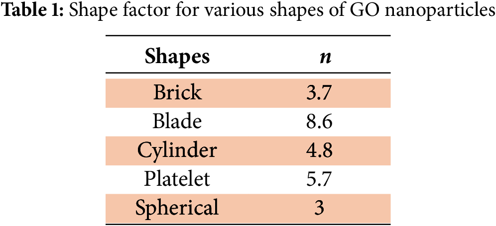
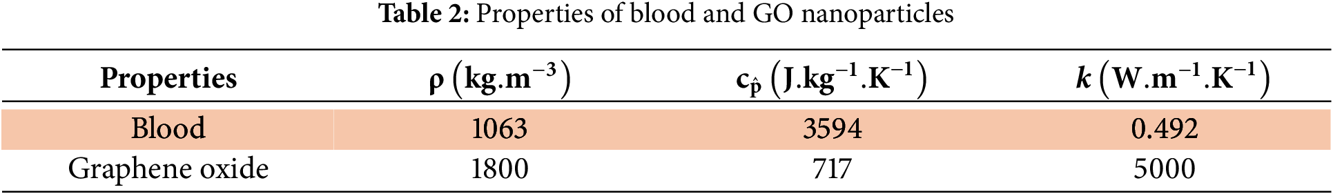
| Temperature | |
| Ambient temperature | |
| Wall temperature | |
| Viscosity variation exponent | |
| Variable viscosity parameter | |
| Pressure | |
| Cartesian coordinates along the stretching surface | |
| Cartesian coordinates normal to stretching surface | |
| Specific heat | |
| Thermal conductivity | |
| Prandtl number | |
| Greek Symbols | |
| Solid volume fraction of nanoparticles | |
| Reference viscosity | |
| Kinematics viscosity | |
| Density | |
| Thermal diffusivity | |
| Obliqueness of the flow | |
| Dynamic viscosity | |
| Velocity slip parameter | |
| Subscripts | |
| Base fluid | |
| Nanoparticles | |
| Nanofluid | |
Nanofluids are fluids that contain nanoparticles, which are particles at the nanometer scale. These fluids are colloidal suspensions of nanoparticles, typically composed of oxides, metals, and carbides. Nanofluids possess unique properties that make them valuable in various heat transfer applications, such as in microelectronics, fuel cells, pharmaceutical processes, hybrid engines, engine cooling/vehicle thermal management, household refrigerators, radiators, and more. Some key research areas involving nanofluids include studies on the impact of physical parameters on their thermal conductivity. For example, Jang et al. [1] focused on how these parameters affect nanofluid conductivity and were the first to model the Brownian motion-induced nano convection, highlighting its significance as a crucial mechanism at the nanoscale. Li et al. [2] concentrated on the advancement of nanofluids, exploring their synthesis and characterization in stationary conditions. Aybar et al. [3] examined the thermal conductivity of nanofluids, highlighting the influence of factors like temperature, and explored mechanisms that enhance thermal conductivity, such as Brownian motion. Tabassum et al. [4] investigated the impact of variable viscosity on the flow characteristics of inclined nanofluid flows containing copper nanoparticles. It was found that the viscosity parameter leads to a decrease in the surface friction coefficient. Arshad et al. [5] conducted a comprehensive study of graphene-based nanofluids: synthesis, analysis, and various applications. They also studied the changes in the behavior of nano-sized graphene particles in different carrier fluids. Hatami et al. [6] discussed the theories of various suspension nanoparticles. Various researchers observed an increase in thermal conductivity after adding nanoparticles. Hatami et al. [7] analyzed the practical applications of nanofluids through experimental and numerical analysis. They focused on cooling and heating applications, i.e., micro-ducts and heating and air conditioning models. Li et al. [8] conducted a comprehensive study from three aspects, i.e., influencing factors, prediction models, and practical applications.
In fluid mechanics, a stagnation point refers to a point on a surface where the velocity is zero. The flow around this point is known as stagnation flow. Oblique stagnation flow occurs when the fluid approaches the surface at an acute angle. Flow over an expanding surface refers to the flow exiting a slot, which can be modeled as a boundary layer emerging from the slot. Viscosity, which depends on temperature, has different relationships for different substances: for liquids, viscosity decreases as temperature increases, while for solids, it increases with temperature. The skin friction coefficient represents the resistance an object experiences from a surface it contacts, defined as the ratio of the frictional force to the normal force. Heat flux is the rate at which heat is transferred from a hotter area to a cooler one through a material over a given time. Researchers have studied stagnation points in various contexts, such as Reza et al. [9], who investigated the oblique stagnation point flow of a two-dimensional stationary incompressible viscous fluid towards a slender boundary, noting that the distance from the stagnation point is directly influenced by velocity, and shear force is inversely proportional to the zero velocity point. Mahapatra et al. [10] also studied the two-dimensional stationary oblique stagnation point flow of an incompressible viscous fluid towards a slender surface. The extended studies on stagnation point flow can be assessed in Refs. [11–13]. Ghaffar [14] discussed the stagnation flow in the oblique geometry of a Newtonian suspension on various boundaries, including stretching sheet, vertical surface, and shrinking sheet. Special effects of germane parameters are noticed and the results of the transformed equations are compared with exact solutions. Lok et al. [15] investigated the magneto-hydrodynamic flow impinging on an extensible surface, the impression of MHD upon flow is noted by a displacement in the stagnation line. Specifically, when dealing with a shrinking surface, there’s an observation of a reversed flow region close to the wall. This suggests that MHD influences not only the stagnation line but also induces a distinct reversed flow zone near the wall when the surface is shrinking. Ghaffari et al. [16] researched the effects of non-linear radiation on the slanting stagnation flow of Maxwell fluid. The study elucidates a notable correlation between temperature and thermal transport rate. Moreover, it demonstrates the direct relationship between a physical parameter, i.e., Prandtl number and heat transfer rate Bano et al. [17] discussed the slanted stagnation flow of a dense fluid with thermal transfer towards an extended cylinder. It explains how the fluid influences obliquely upon the surface of the cylinder. The graphical representation of temperature and velocity profiles are illustrated and further examined for the effects of related parameters.
A very important property of fluids that plays a vital role in the flow regime is viscosity. Viscosity depends strongly on temperature. In liquids, it depicts an inverse relationship with temperature whereas a direct relationship with temperature is observed in gases. Temperature dependence on viscosity is important for various applications e.g., Increase in temperatures causes an increase in the attractive forces between particles which helps them to overcome the surrounding forces. A daily life example is cooking oil moving more fluidly in hot utensils than in a cold one. Here are a few explorations in which viscosity variation is studied. Booker [18] explored thermal convection in fluids with viscosity that is highly dependent on temperature. They examined the effects on both free and rigid boundaries, observing that the flow is three-dimensional at a free upper boundary, while it is nearly two-dimensional with a rigid upper boundary. Wall et al. [19] investigated the linear stability of channel flow in fluids with temperature-dependent viscosity, focusing on three material effects: bulk effects, velocity-profile shape effects, and thin-layer effects. Nguyen et al. [20] examined viscosity variations in water-based nanofluids based on temperature and particle size, applying the phenomena of Couette flow to a viscometer for their results. Prasad et al. [21] studied the impact of variable viscosity on magnetohydrodynamic (MHD) viscoelastic fluid flow and heat transfer over a stretching sheet, finding that an increase in the magnetic field parameter leads to a decrease in the temperature profile. They also identified an inverse relationship between skin friction and magnetic field parameters. Anjali Devi et al. [22] investigated the effects of temperature-dependent viscosity and thermal conductivity on hydromagnetic flow, focusing on physical parameters such as skin friction coefficient, temperature, velocity, and heat transfer rates. Huda et al. [23] analyzed temperature-dependent viscosity in nanofluids with shape factors over a heated tube, finding that the velocity of the nanofluid increased. Alabdan et al. [24] examined the flow of a couple stress nanofluid over an oscillatory stretching surface, noting temperature changes in viscosity and thermal Biot numbers, and observing that the skin friction coefficient periodically increased with the viscosity vector and couple stress parameter. Ahmad et al. [25] stressed the relationships between viscosity as a function of temperature, thermal conductivity, and exothermic catalytic processes. In the context of these chemical interactions, the parameters have a significant impact on temperature distribution, mass concentration patterns, and velocity profiles.
The shape factor of nanoparticles is a measure of their geometry or form, which affects their interaction with the surrounding fluid. For instance, nanoparticles can have different shapes spherical, rod-like (elongated), plate-like, or other complex forms. Each shape influences how the nanofluid behaves, such as how it conducts heat, flows, or interacts with surfaces. Shape factors often refer to geometric parameters or characteristics of nanoparticles dispersed within the fluid. These factors can influence the heat transfer, rheological properties, and behavior of the nanofluid. Shape factors play a vital role in modeling the thermal conductivity, viscosity, and other properties of nanofluids. Researchers frequently consider these factors when studying and designing nanofluids for various applications, ranging from electronic cooling to biomedical treatments, as different shapes can lead to varying performance characteristics. Several studies have explored viscosity variation in nanofluids. Sheikholeslami et al. [26] examined the effect of shape factors on nanofluids in a porous medium, finding that the Hartmann number is inversely related to the nanofluid velocity and Nusselt number. Waqas et al. [27] highlighted the significance of shape factors in Sisko nanofluids, with their results showing that the velocity profile decreases as the velocity slip parameter increases. Additionally, the temperature profile of the nanofluids increases with both the thermal radiation parameter and the nanoparticle volume fraction. Hayat et al. [28] investigated the impact of particle shape on flow and heat transfer, offering an extensive discussion on the influence of various factors such as unsteadiness, magnetic parameter, and Eckert number. Both velocity and temperature are affected by the shape of nanoparticles, which leads to optimal flow and heat transfer.
Velocity slip highlights the discrepancy in velocity between a fluid and its solid boundary. Discrepancy means that the fluid that adjacent to the solid surface does not stick to it but rather shows relative motion with it. Velocity slip is strongly impacted by fluid traits, boundary features, and flow dynamics. Practically, its vital comprehension extends to microfluidics and rarefied gas analysis, challenging conventional presumptions. Integrating slip velocity into predictive frameworks enables more nuanced understandings of fluid behavior, driving innovation in practical domains. Here are some areas of exploration in which velocity slip condition is studied. Khan et al. [29] emphasized the study of phase flow characteristics in MHD nanofluids, incorporating the effects of slip on oscillatory slanted stagnation flow under an inclined magnetic field. His study compared the behaviors of nanoparticles made of Copper, Alumina, and Titania, using water as the carrier fluid, and found that copper nanoparticles enhanced the magnetic susceptibility of the nanofluid. Rizwana et al. [30] explored the slip effects on time-independent tilted stagnation point flow of nanofluids under an oblique magnetic field, observing that the Casson fluid parameter accelerates fluid motion. Additionally, Joule heating and dissipation were found to raise the system’s temperature. Kolsi et al. [31] focused on the thermal development of ethylene glycol-based material by adding a hybrid nanofluid for slip flow at an oblique stagnation point, noting a strong influence of slip intensity on temperature and velocity profiles. Mandal et al. [32] conducted a numerical simulation on mixed convective and arbitrary oblique stagnation point slip flow of an MHD fluid, revealing that the magnetic field amplifies skin friction as flow obliqueness increases. Bai et al. [33] studied the variable MHD oblique stagnation slip flow of nanofluids, incorporating the Cattaneo-Christov double diffusion and Buongiorno models, and observed that nanoparticle diffusion, through thermophoresis and Brownian motion, affects concentration and energy and mass transfer, with advection and radiation aiding thermal transmission. Rahman et al. [34] examined the oblique stagnation-point flow of a nanofluid past a shrinking sheet, noting that shrinking parameters and dimensionless strain rates shift the point of zero skin friction on a stretching sheet, with increasing strain rate leading to oblique flow towards the surface. Their study also suggested the existence of dual solutions for the opposing flow case. Abbas et al. [35] studied the stagnation flow of a micropolar nanofluid past a circular cylinder with velocity and thermal slip, finding that copper-water nanofluids exhibited the highest skin friction and heat transfer rates compared to titanium-water and alumina-water nanofluids.
Benkhedda et al. [36] presented a numerical investigation of time-independent forced convective heat transfer and fluid flow of a hybrid nanofluid through an isothermally heated flat tube, considering various nanoparticle shapes. Using the finite volume method in cylindrical coordinates and solving with a FORTRAN program, their study found that platelet-shaped nanoparticles yielded the highest friction factor values, especially at volume fractions ranging from 0% to 8%. Kata et al. [37] examined the enhanced thermal characteristics of a hybrid nanofluid composed of Al2O3 (alumina) and Ag (silver) nanoparticles suspended in a 50%–50% mixture of C2H6O2-H2O, impacting obliquely on an elastic surface under a magnetic field. They found that the thermal energy transfer rate in the hybrid nanofluid increased by 11.5% compared to spherical particles when using blade-shaped nanoparticles. Li et al. [38] investigated the effect of the shape factor on a mass-based hybrid nanofluid model for Homann stagnation-point flow in porous media, using the HAM-based Mathematica package BVPh 2.0 to approximate solutions for coupled nonlinear ordinary differential equations. Their results showed that platelet-shaped nanoparticles in the hybrid nanofluid model produced the highest heat transfer rates and minimal surface friction, with skin friction coefficient values ranging from 2.03443 to 3.10222 depending on the permeability coefficient. Rafique et al. [39] studied the influence of nanoparticle shapes on the entropy production of a water-alumina nanofluid flowing over a permeable, MHD stretching sheet with quadratic velocity profiles, factoring in viscous dissipation and Joule heating effects. Their results indicated a 6.3% increase in wall shear stress as nanoparticle volume fraction increased from 0% to 2%, with further increases as the fraction rose from 2% to 4%. Additionally, when the magnetic effect accounted for about 5% of the boundary layer flow, the convective heat transfer rate increased by approximately 16.4%. Rosalind Mary et al. [40] explored the thermal applications of magnetized hybrid nanomaterials by evaluating the effects of different nanoparticle shapes. Their study, using a 50:50 mixture of ethylene glycol (C2H6O2) and water (H2O) with silver and alumina nanoparticles, showed that both mono and hybrid nanofluid temperature profiles increased with nanoparticle volume fraction and Biot number.
Carbon-based nanomaterial GO has unique properties such as high surface area, excellent conductivity, and the ability to interact with biological systems. In thermal therapy and drug delivery, graphene oxide-based nanofluids are injected into the bloodstream to deliver drugs or thermal energy to tumors. The shape of graphene oxide nanoparticles in nanofluids significantly influences the flow characteristics and fluid dynamics properties. By modifying the shape of the graphene oxide, we can optimize nanofluid thermal efficiency. The viscosity of a fluid, particularly one containing suspended nanoparticles such as graphene oxide, varies with temperature. Understanding how viscosity changes with temperature is essential for analyzing heat transfer in dynamic systems. This temperature dependence affects the fluid’s flow behavior and heat thermal efficiency. The existing research on oblique nanofluid flows conveys that less consideration has been paid to towards investigation of the heat transport phenomenon influenced by viscosity variation and various shape features of GO nanoparticles. In the current exploration we are aiming to study the influence of variation in GO nanoparticle shapes and viscosity upon the heat transport characteristics and velocity profile of blood based oblique nanofluid flow in neighborhood of stagnation-point that has not been investigated before.
Although significant research has been conducted on the analysis of nanoparticles shape factors, limited studies have investigated the heat transfer behavior in oblique stagnation point flow influenced by these shape factors. This study seeks to examine this concept more thoroughly by addressing the following questions:
• What effects do different nanoparticle shapes have on both primary and secondary flow profiles, as well as temperature distribution?
• How do variations in porosity and viscosity affect the flow characteristics?
We are taking a stationary state, 2D non-compressible, non-aligned transport of blood-based nanofluid containing graphene oxide nano-sized particles with viscosity depending upon the temperature in the vicinity of the stagnation point. Nanofluid strikes the stretching surface obliquely and occupies the region above the horizontal axis. Here blood is used as a carrier liquid and its viscosity changes substantially with temperature variation, therefore modified form of (the Brinkman) viscosity model is incorporated to examine the viscosity varying with respect to temperature. The nanoparticles different shapes play a crucial role in determining the heat transfer properties of nanofluids for that reason different shapes of GO nanoparticles of size 25 nm are added to improve the heat transfer performance. Two opposing forces of equal magnitude are plotted on
where
where

Figure 1: Physical description of the flow problem
Respective boundary conditions are [4]
Since the nanofluids are more likely to exhibit the slip condition at the stretching boundary, that is why the velocity slip condition is employed for accurately describing the velocity profile in the boundary layer. In Eq. (8),
where
Employing Eq. (10), in Eqs. (1)–(4) and (8), (9), their non-dimensional forms are
where
Differentiating Eq. (18) w.r.t
Subtracting Eqs. (23) from (24) and eliminating
Revising the stream function as
where
where
Here
Introducing
Using Eqs. (36) in (35) and surface conditions in (31)
Prominent system variables such as shearing force and thermal flux at the extended surface in dimensionless form are
Stagnation point is given by
The final boundary value problem is represented by a system of three ODEs (ordinary differential equations) of total order seven: Eq. (34) (third-order normal momentum), Eq. (37) (reduced second-order tangential momentum), and Eq. (28) (second-order temperature), along with their boundary conditions from Eq. (31) modified by the replacement conditions in Eq. (38). Solving this system analytically is extremely challenging, if not entirely unfeasible. Therefore, a computational approach is adopted, using numerical quadrature (specifically, a shooting algorithm) combined with the robust Runge-Kutta Fehlberg method. The approximate CPU time for this execution is 10−1 s. Various schemes [41–43] are available to solve fluid flow problems but this approach can easily handle multi-order ordinary differential boundary value problems (BVPs) and has been implemented in various studies using different symbolic codes. Its main advantage is its stability when applied to stiff equations. This method [44] uses an efficient procedure to determine an appropriate step size of h = 0.0001 for stepping. Two different approximations are made for the solution and compared, with the step size being considered acceptable if the results are in strong agreement.
Otherwise, the process is repeated with a smaller step size. Following six values are required in each step:
Using RK 4th order scheme, the I.V.P is approximated as
By applying the following substitutions in Eqs. (25), (27), and (30), the final system of three coupled ordinary differential equations of total order seven, along with the modified boundary conditions in (26) and (31), is obtained.
The following system of differential equations, which defines the transformed three flow variables (the two linear velocity components and temperature), is then derived:
where
Here
The primary goal of this study is to assess the thermal performance of a nanofluid (GO-Blood) under the influence of different factors, including the shape factor of nanoparticles and the temperature-dependent viscosity parameter, stretching ratio parameter and velocity slip parameter. The nanofluid is composed of Graphene oxide dispersed in a base liquid blood. The study examines how the enhanced thermal (physical) properties of the nanofluid influence the velocity and temperature distributions within the fluid, as well as the friction drag coefficient and heat transfer rate. The graphical results achieved by the numerical scheme are presented through Figs. 2 to 18. Nanoparticle concentration is considered

Figure 2:

Figure 3:
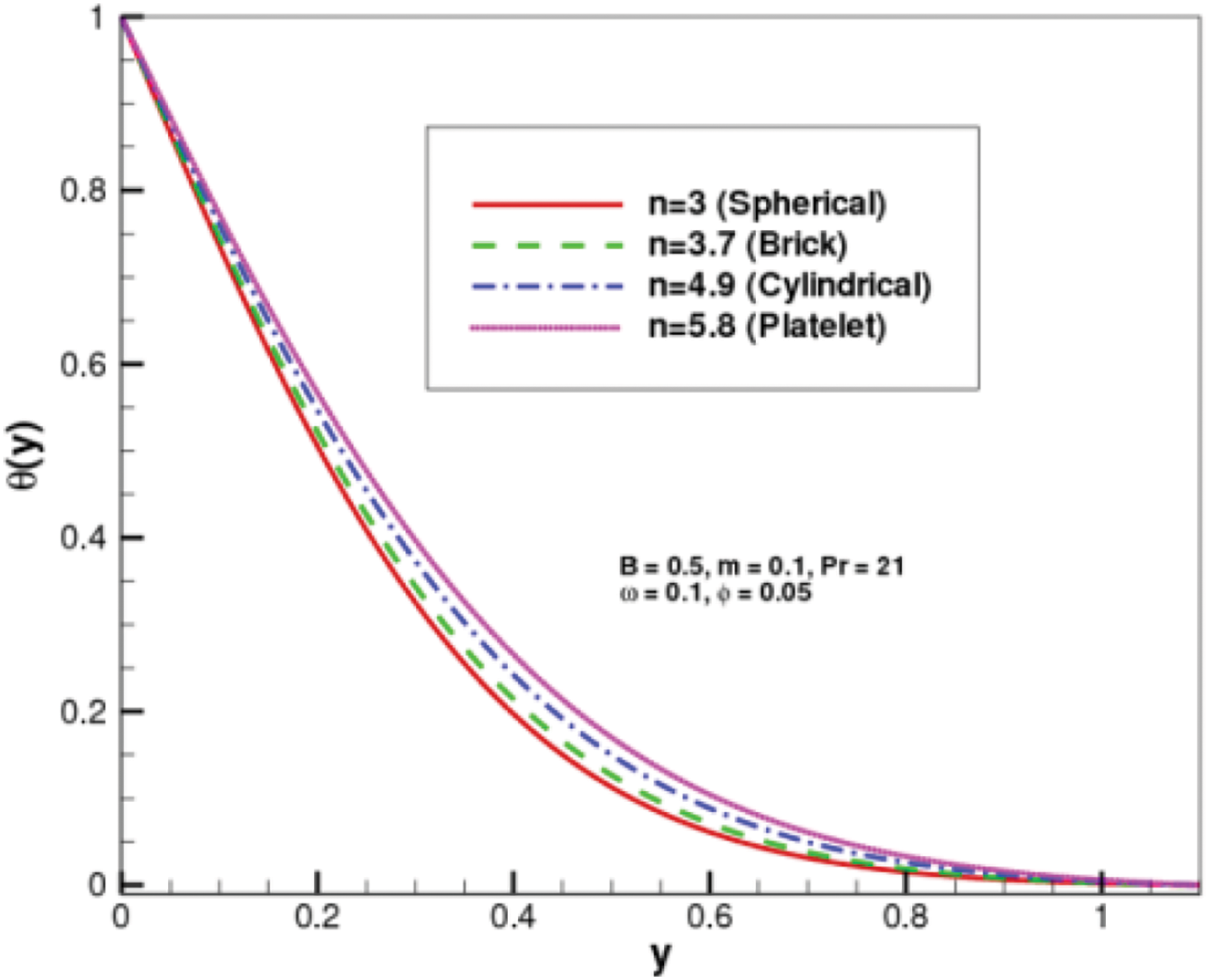
Figure 4:

Figure 5:

Figure 6:
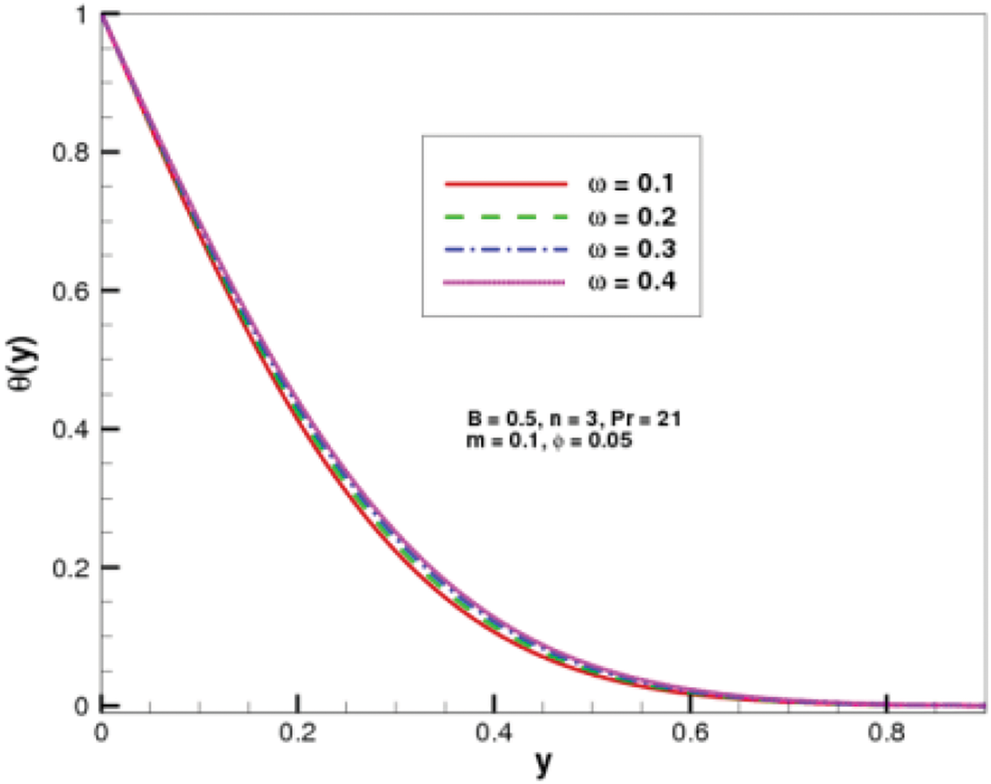
Figure 7:
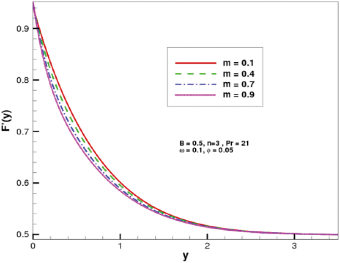
Figure 8:

Figure 9:
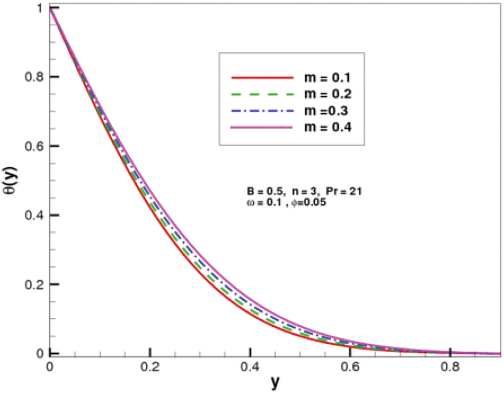
Figure 10:

Figure 11:
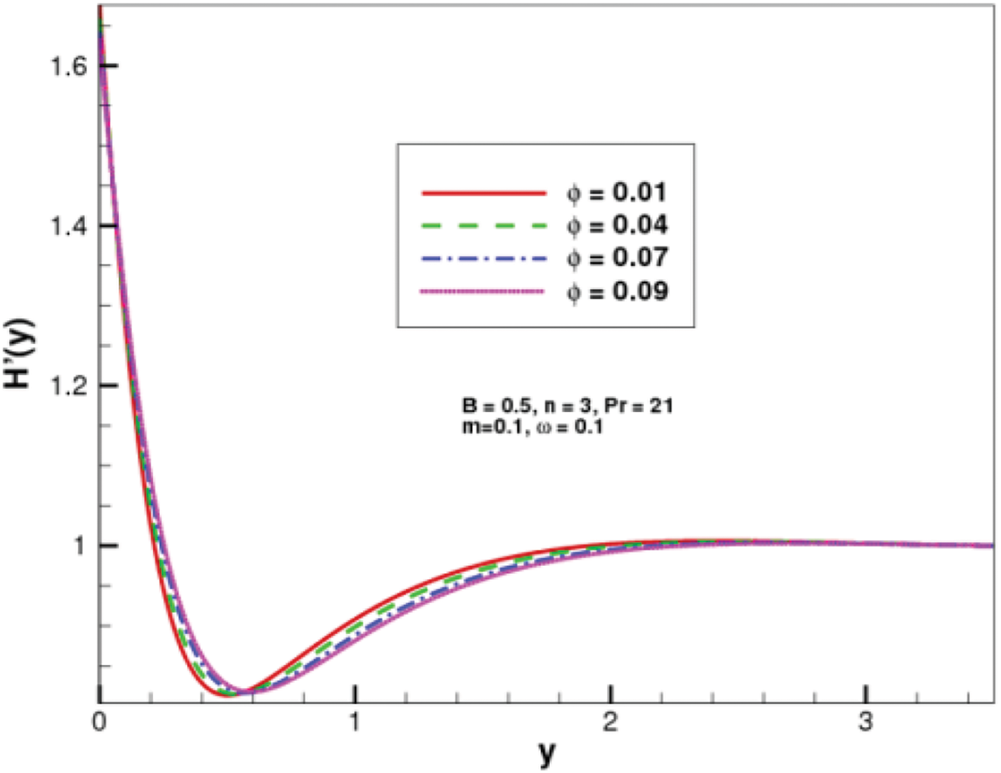
Figure 12:

Figure 13:

Figure 14:

Figure 15:

Figure 16:

Figure 17: Impact of various shapes of nanoparticles on thermal conductivity of nanofluid

Figure 18: Heat transfer rate when varying the nanoparticles shapes
Figs. 5 and 6 are presented to examine the effect of the velocity slip parameter on both velocity profiles. The graphs indicate that an increase in the slip parameter
Figs. 8 and 9 are plotted to inspect the influence of viscosity variation parameter
Fig. 10 shows that growing values of
These include enhanced heat transfer, improved momentum transfer by the nanoparticles, possible reductions in flow resistance (depending on changes in viscosity), and alterations to the boundary layer thickness. Together, these effects facilitate more efficient fluid motion, leading to an increase in both velocity components near the surface. Fig. 13 is indicating in increasing trend in temperature distribution with respect to nanoparticles volume fraction
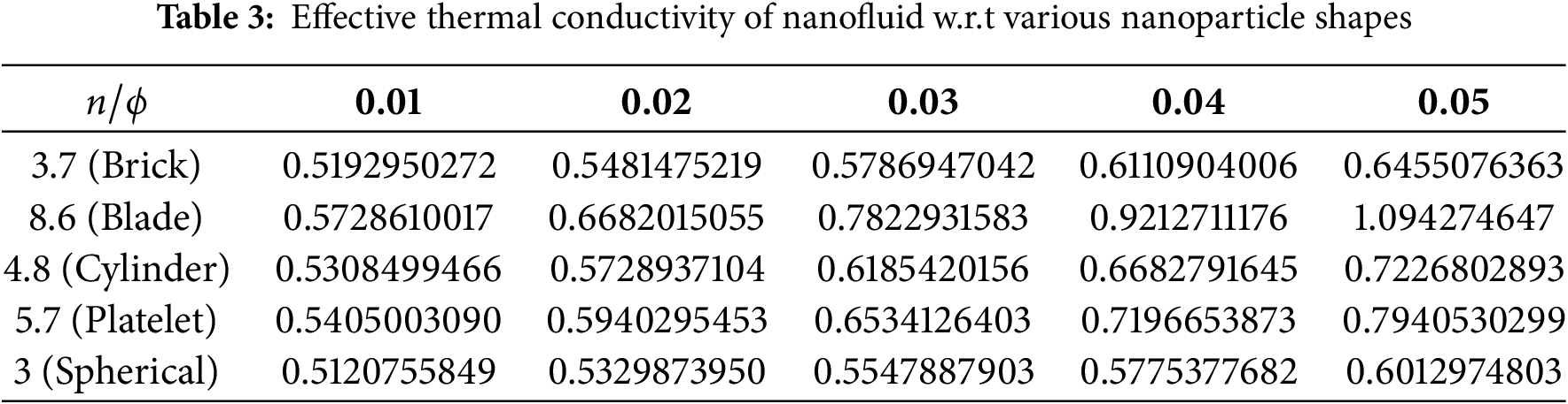

Figure 19: Normal component of skin friction for

Figure 20: Tangential component of skin friction for
The normal skin friction coefficient represents the resistance the fluid experiences in the direction perpendicular to the surface at the stagnation point. As the nanoparticle volume fraction rises, the fluid’s effective viscosity increases, which tends to lessen the velocity gradients near the surface in the normal direction. This increased viscosity results in a smoother transition in velocity perpendicular to the surface, thereby reducing the resistance in the normal direction. Tangential skin friction refers to the resistance in the direction parallel to the surface. As the nanoparticle concentration increases, the fluid’s viscosity rises, which can enhance the shear stress near the surface. Higher viscosity generally results in a thicker boundary layer, leading to greater tangential friction, as the fluid’s velocity within the boundary layer encounters more resistance. Streamline patterns for stretching ratio parameter
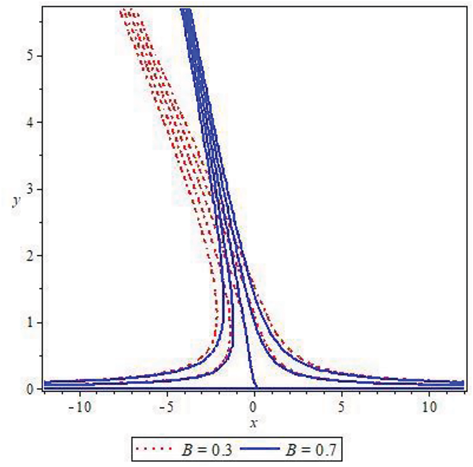
Figure 21: Streamlines for stretching ratio constant

Figure 22: Streamlines for constant and variable viscosity
A blood-based non-aligned stagnation point flow with graphene oxide nanoparticles has been studied under the influence of various shapes of nanoparticles. The numerical outcomes of the governing equations are:
• The normal velocity profile is showing maximum velocity with spherical and the minimum velocity with platelet shape of nanoparticles.
• Maximum temperature distribution is achieved with blade shape. It is also seen that the temperature profile enhanced significantly by increasing nanoparticle volume fraction from 1% to 9%.
• The effects of increasing the slip parameter
• Variable viscosity varies directly with viscous fluid and inversely with normal velocity.
• Nanoparticle volume fraction has an increasing effect on heat flux, and the highest thermal conductivity is achieved for blade-shaped nanoparticles.
• The normal drag coefficient has an increasing trend and the longitudinal friction coefficient has a decreasing trend with respect to the slip parameter.
• Streamline patterns are more inclined towards left for the stretching ratio parameter
While this study offers important insights into heat transfer enhancement in blood-based oblique nanofluid flow by varying nanoparticle shapes and fluid viscosity concerning temperature, exploring the effects of unsteady (time-dependent) nanofluid flow under the assumptions made in this study would be an intriguing direction for future research.
Acknowledgement: The authors would like to thank Prince Sultan University, Saudi Arabia, for the technical support through the TAS Research Lab.
Funding Statement: The authors received no specific funding for this study.
Author Contributions: Rabil Tabassum: Modeling, methodology, manuscript preparation, supervision and review. M. Kamran: Literature review, methodology and graphical results. Khalil Ur Rehman: Validation, interpretation of results and review. Wasfi Shatanawi: Writing—review and editing. Rashid Mehmood: Review and editing. All authors reviewed the results and approved the final version of the manuscript.
Availability of Data and Materials: The data that support the findings of this study are available from the corresponding author upon reasonable request.
Ethics Approval: Not applicable.
Conflicts of Interest: The authors declare no conflicts of interest to report regarding the present study.
References
1. Jang SP, Choi SUS. Effects of various parameters on nanofluid thermal conductivity. J Heat Transf. 2007;129(5):617–23. doi:10.1115/1.2712475. [Google Scholar] [CrossRef]
2. Li Y, Zhou JE, Tung S, Schneider E, Xi S. A review on development of nanofluid preparation and characterization. Powder Technol. 2009;196(2):89–101. doi:10.1016/j.powtec.2009.07.025. [Google Scholar] [CrossRef]
3. Aybar HŞ, Sharifpur M, Azizian MR, Mehrabi M, Meyer JP. A review of thermal conductivity models for nanofluids. Heat Transf Eng. 2015;36(13):1085–110. doi:10.1080/01457632.2015.987586. [Google Scholar] [CrossRef]
4. Tabassum R, Mehmood R, Pourmehran O, Akbar N, Gorji-Bandpy M. Impact of viscosity variation on oblique flow of Cu-H2O nanofluid. J Process Mech Eng. 2018;232(5):622–31. doi:10.1177/0954408917732759. [Google Scholar] [CrossRef]
5. Arshad A, Jabbal M, Yan Y, Reay D. A review on graphene based nanofluids: preparation, characterization and applications. J Mol Liq. 2019;279:444–84. doi:10.1016/j.molliq.2019.01.153. [Google Scholar] [CrossRef]
6. Hatami M, Jing D. Introduction to nanofluids. In: Nanofluids. Amsterdam: Elsevier; 2020. p. 1–50. doi: 10.1016/b978-0-08-102933-6.00001-9. [Google Scholar] [CrossRef]
7. Hatami M, Jing D. Nanofluid analysis in different applications. In: Nanofluids. Amsterdam: Elsevier; 2020. p. 283–347. doi:10.1016/b978-0-08-102933-6.00006-8. [Google Scholar] [CrossRef]
8. Li J, Zhang X, Xu B, Yuan M. Nanofluid research and applications: a review. Int Commun Heat Mass Transf. 2021;127:105543. doi:10.1016/j.icheatmasstransfer.2021.105543. [Google Scholar] [CrossRef]
9. Reza M, Gupta AS. Steady two-dimensional oblique stagnation-point flow towards a stretching surface. Fluid Dyn Res. 2005;37(5):334–40. doi:10.1016/j.fluiddyn.2005.07.001. [Google Scholar] [CrossRef]
10. Mahapatra TR, Dholey S, Gupta AS. Oblique stagnation-point flow of an incompressible visco-elastic fluid towards a stretching surface. Int J Non Linear Mech. 2007;42(3):484–99. doi:10.1016/j.ijnonlinmec.2007.01.008. [Google Scholar] [CrossRef]
11. Li D, Labropulu F, Pop I. Oblique stagnation-point flow of a viscoelastic fluid with heat transfer. Int J Non Linear Mech. 2009;44(10):1024–30. doi:10.1016/j.ijnonlinmec.2009.07.007. [Google Scholar] [CrossRef]
12. Ishak A, Jafar K, Nazar R, Pop I. MHD stagnation point flow towards a stretching sheet. Phys A Stat Mech Appl. 2009;388(17):3377–83. doi:10.1016/j.physa.2009.05.026. [Google Scholar] [CrossRef]
13. Mustafa M, Hayat T, Pop I, Asghar S, Obaidat S. Stagnation-point flow of a nanofluid towards a stretching sheet. Int J Heat Mass Transf. 2011;54(25–26):5588–94. doi:10.1016/j.ijheatmasstransfer.2011.07.021. [Google Scholar] [CrossRef]
14. Ghaffar A. Oblique stagnation point flows [master’s theses]. Regina, SK, Canada: Faculty of Graduate Studies and Research, University of Regina; 2012. [Google Scholar]
15. Lok YY, Merkin JH, Pop I. MHD oblique stagnation-point flow towards a stretching/shrinking surface. Meccanica. 2015;50(12):2949–61. doi:10.1007/s11012-015-0188-y. [Google Scholar] [CrossRef]
16. Ghaffari A, Javed T, Mustafa I. Non-linear radiation influence on oblique stagnation point flow of Maxwell fluid. Rev Mex Fís. 2018;64(4 Jul–Aug):420–8. doi:10.31349/RevMexFis.64.420. [Google Scholar] [CrossRef]
17. Bano A, Sajid M, Mahmood K, Rana MA. An oblique stagnation point flow towards a stretching cylinder with heat transfer. Phys Scr. 2020;95(1):015704. doi:10.1088/1402-4896/ab4772. [Google Scholar] [CrossRef]
18. Booker JR. Thermal convection with strongly temperature-dependent viscosity. J Fluid Mech. 1976;76(4):741–54. doi:10.1017/S0022112076000876. [Google Scholar] [CrossRef]
19. Wall DP, Wilson SK. The linear stability of channel flow of fluid with temperature-dependent viscosity. J Fluid Mech. 1996;323:107–32. doi:10.1017/S0022112096000869. [Google Scholar] [CrossRef]
20. Nguyen CT, Desgranges F, Roy G, Galanis N, Maré T, Boucher S, et al. Temperature and particle-size dependent viscosity data for water-based nanofluids-Hysteresis phenomenon. Int J Heat Fluid Flow. 2007;28(6):1492–506. doi:10.1016/j.ijheatfluidflow.2007.02.004. [Google Scholar] [CrossRef]
21. Prasad KV, Pal D, Umesh V, Prasanna Rao NS. The effect of variable viscosity on MHD viscoelastic fluid flow and heat transfer over a stretching sheet. Commun Nonlinear Sci Numer Simul. 2010;15(2):331–44. doi:10.1016/j.cnsns.2009.04.003. [Google Scholar] [CrossRef]
22. Anjali Devi SP, Prakash M. Temperature dependent viscosity and thermal conductivity effects on hydromagnetic flow over a slendering stretching sheet. J Niger Math Soc. 2015;34(3):318–30. doi:10.1016/j.jnnms.2015.07.002. [Google Scholar] [CrossRef]
23. Huda AB, Akbar NS. Heat transfer analysis with temperature-dependent viscosity for the peristaltic flow of nano fluid with shape factor over heated tube. Int J Hydrog Energy. 2017;42(39):25088–101. doi:10.1016/j.ijhydene.2017.08.054. [Google Scholar] [CrossRef]
24. Alabdan R, Khan SU, Al-Qawasmi AR, Vakkar A, Tlili I. Applications of temperature dependent viscosity for Cattaneo-Christov bioconvection flow of couple stress nanofluid over oscillatory stretching surface: a generalized thermal model. Case Stud Therm Eng. 2021;28:101412. doi:10.1016/j.csite.2021.101412. [Google Scholar] [CrossRef]
25. Ahmad U, Ashraf M, Al-Zubaidi A, Ali A, Saleem S. Effects of temperature dependent viscosity and thermal conductivity on natural convection flow along a curved surface in the presence of exothermic catalytic chemical reaction. PLoS One. 2021;16(7):e0252485. doi:10.1371/journal.pone.0252485. [Google Scholar] [PubMed] [CrossRef]
26. Sheikholeslami M, Shamlooei M. Magnetic source influence on nanofluid flow in porous medium considering shape factor effect. Phys Lett A. 2017;381(36):3071–8. doi:10.1016/j.physleta.2017.07.028. [Google Scholar] [CrossRef]
27. Waqas H, Farooq U, Muhammad T, Manzoor U. Importance of shape factor in Sisko nanofluid flow considering gold nanoparticles. Alex Eng J. 2022;61(5):3665–72. doi:10.1016/j.aej.2021.09.010. [Google Scholar] [CrossRef]
28. Hayat U, Shaiq S, Shahzad A, Khan R, Kamran M, Ali Shah N. The effect of particle shape on flow and heat transfer of Ag-nanofluid along stretching surface. Chin J Phys. 2023;85:708–21. doi:10.1016/j.cjph.2023.02.008. [Google Scholar] [CrossRef]
29. Khan AU, Nadeem S, Hussain ST. Phase flow study of MHD nanofluid with slip effects on oscillatory oblique stagnation point flow in view of inclined magnetic field. J Mol Liq. 2016;224:1210–9. doi:10.1016/j.molliq.2016.10.102. [Google Scholar] [CrossRef]
30. Rizwana R, Hussain A, Nadeem S. Slip effects on unsteady oblique stagnation point flow of nanofluid in a view of inclined magnetic field. Math Probl Eng. 2020;2020:6580409. doi:10.1155/2020/6580409. [Google Scholar] [CrossRef]
31. Kolsi L, Abbasi A, Alqsair UF, Farooq W, Omri M, Khan SU. Thermal enhancement of ethylene glycol base material with hybrid nanofluid for oblique stagnation point slip flow. Case Stud Therm Eng. 2021;28:101468. doi:10.1016/j.csite.2021.101468. [Google Scholar] [CrossRef]
32. Mandal PK, Seth GS, Sarkar S, Chamkha A. A numerical simulation of mixed convective and arbitrarily oblique radiative stagnation point slip flow of a CNT-water MHD nanofluid. J Therm Anal Calorim. 2021;143(3):1901–16. doi:10.1007/s10973-020-10344-3. [Google Scholar] [CrossRef]
33. Bai Y, Tang Q, Zhang Y. Unsteady MHD oblique stagnation slip flow of Oldroyd-B nanofluids by coupling Cattaneo-Christov double diffusion and Buongiorno model. Chin J Phys. 2022;79:451–70. doi:10.1016/j.cjph.2022.09.013. [Google Scholar] [CrossRef]
34. Rahman MM, Grosan T, Pop I. Oblique stagnation-point flow of a nanofluid past a shrinking sheet. Int J Numer Meth Heat Fluid Flow. 2016;26(1):189–213. doi:10.1108/HFF-10-2014-0315. [Google Scholar] [CrossRef]
35. Abbas N, Saleem S, Nadeem S, Alderremy AA, Khan AU. On stagnation point flow of a micro polar nanofluid past a circular cylinder with velocity and thermal slip. Results Phys. 2018;9:1224–32. doi:10.1016/j.rinp.2018.04.017. [Google Scholar] [CrossRef]
36. Benkhedda M, Boufendi T, Tayebi T, Chamkha AJ. Convective heat transfer performance of hybrid nanofluid in a horizontal pipe considering nanoparticles shapes effect. J Therm Anal Calorim. 2020;140(1):411–25. doi:10.1007/s10973-019-08836-y. [Google Scholar] [CrossRef]
37. Kata S, Ganganapalli S, Kuppalapalle V. Transport of thermal energy in the magnetohydrodynamic oblique stagnation point flow in a hybrid nanofluid with nanoparticle shape effect. Heat Trans. 2022;51(5):4331–48. doi:10.1002/htj.22502. [Google Scholar] [CrossRef]
38. Li S, You X. Shape-factor impact on a mass-based hybrid nanofluid model for homann stagnation-point flow in porous media. Nanomater. 2023;13(6):984. doi:10.3390/nano13060984. [Google Scholar] [PubMed] [CrossRef]
39. Rafique K, Mahmood Z, Alqahtani H, Eldin SM. Various nanoparticle shapes and quadratic velocity impacts on entropy generation and MHD flow over a stretching sheet with joule heating. Alex Eng J. 2023;71:147–59. doi:10.1016/j.aej.2023.03.021. [Google Scholar] [CrossRef]
40. Rosalind Mary GL, Sreelakshmi K, Adnan, Khan SU, Mir A, Alshammari BM, et al. Applications of nonlinear thermal radiation on performance of hybrid nanofluid (Al2O3-Ag)/(C2H6O2-H2O) for stagnation point flow: Blade and spherical shaped nanoparticles. J Radiat Res Appl Sci. 2024;17(4):101171. doi:10.1016/j.jrras.2024.101171. [Google Scholar] [CrossRef]
41. Asghar Z, Khan MWS, Gondal MA. Numerical analysis of Carreau fluid inside a horizontal passage with axial conduction and viscous dissipation: an extended Graetz problem. J Therm Anal Calorim. 2024;149(14):7527–35. doi:10.1007/s10973-024-13332-z. [Google Scholar] [CrossRef]
42. Baazeem AS, Arif MS, Abodayeh K. An efficient and accurate approach to electrical boundary layer nanofluid flow simulation: A use of artificial intelligence. Processes. 2023;11(9):2736. doi:10.3390/pr11092736. [Google Scholar] [CrossRef]
43. Nawaz Y, Shoaib Arif M, Abodayeh K, Hassan Soori A. A two-stage multi-step numerical scheme for mixed convective Williamson nanofluid flow over flat and oscillatory sheets. Int J Mod Phys B. 2024;38(22):2450298. doi:10.1142/s0217979224502989. [Google Scholar] [CrossRef]
44. Muhammad K, Alrihieli HF, Allehiany FM, Gamaoun F. Comparative study of stagnation point nanofluid flow with partial slips using shooting technique. J Therm Anal Calorim. 2024;149(4):1715–24. doi:10.1007/s10973-023-12736-7. [Google Scholar] [CrossRef]
Cite This Article
 Copyright © 2025 The Author(s). Published by Tech Science Press.
This work is licensed under a Creative Commons Attribution 4.0 International License , which permits unrestricted use, distribution, and reproduction in any medium, provided the original work is properly cited.
 Downloads
 Citation Tools