
 Submit a Paper
 Propose a Special lssue
 Open Access
ARTICLE

Energy Analysis of the Aircraft Environment Control System Using Air with and without Humidity
1 Aeronautical Engineering Department, Universidad Politécnica Metropolitana de Hidalgo, Tolcayuca, 43860, Hidalgo, Mexico
2 Mechanical Engineering Department, Engineering Division, Universidad de Guanajuato, Salamanca, 36787, Guanajuato, Mexico
3 Departamento de Ingeniería Mecánica, Instituto Tecnológico de la Laguna, Tecnológico Nacional de México, Torreón, 27000, Coahuila, México
4 Ingeniería Mecánica, Escuela Superior de Ciudad Sahagún, Universidad Autónoma del Estado de Hidalgo, Ciudad Sahagún, 43970, Hidalgo, Mexico
5 Division of Graduate Studies and Research, IT de Pachuca, Tecnológico Nacional de México, Pachuca, 42083, Hidalgo, Mexico
* Corresponding Author: J. F. Ituna-Yudonago. Email:
(This article belongs to the Special Issue: Innovative Cooling Systems: Design, Optimization, and Applications)
Frontiers in Heat and Mass Transfer 2025, 23(5), 1365-1393. https://doi.org/10.32604/fhmt.2025.068100
Received 21 May 2025; Accepted 14 August 2025; Issue published 31 October 2025
 View Full Text
 Download PDF
Abstract
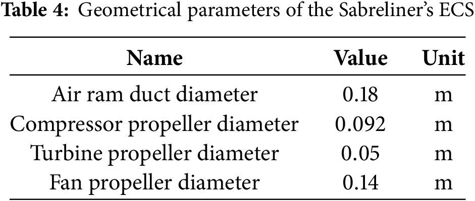
This paper presents a thermophysical study approach for a pure environmental control system (ECS), incorporating the geometric dimensions of heat exchangers, ram air duct, and air cycle machine (ACM) blades of the Sabreliner’s environmental control system. Real flight scenarios are simulated by considering flight input variables such as altitude, aircraft speed, compression ratio of the air cycle machine, and the mass flow rate of bleed air. The study evaluates the coefficient of performance (COP) of the environmental control system, the heat exchanger efficiencies, and the work distribution of the air cycle machine based on five flight scenarios, with a particular focus on considering the effects of humidity on environmental control system performance. The results demonstrate that at cruising altitude (11,000 m), air humidity conditions allow an increase in the COP of around 9.28% compared to dry conditions. Conversely, on land, humidity conditions reduce the performance by 4.26% compared to dry conditions. It was also found that the effects of humidity at high aircraft speeds become negligible. In general terms, the humidity conditions in the air proved to have positive effects on the environmental control system’s performance but negative effects on the heat exchanger efficiencies, reducing them by 0.22%. Additionally, land conditions reflect significant improvements in performance when the compression ratio of the air cycle machine is varied. Furthermore, in the work distribution of the air cycle machine, humidity conditions were demonstrated to consume 2.91% less work from the turbine compared to dry conditions.Keywords
Aircraft are vehicles that, according to a flight mission, experience changes in atmospheric conditions through different phases such as takeoff, ascent, cruise flight, descent, and landing. This means that as the aircraft increases or decreases its altitude, the thermodynamic properties of the atmospheric air vary throughout the entire mission [1]. These variations cause changes in the operating regimes of certain aircraft systems. One of the systems most affected by altitude variation is the Environment control system (ECS). The ECS is responsible for addressing inconsistencies in the pressure and temperature of atmospheric air (which pose challenges to human survival) and providing an artificial climate within the cabin to sustain life under these conditions [2].
The ECS is defined as a group of systems responsible for controlling the pressure, temperature, humidity, and pollutants within an aircraft, ensuring the survival and comfort of the occupants, as well as the integrity of some onboard electrical equipment [3].
The machine used in the ECS can be an air cycle machine (ACM), a vapor cycle machine (VCM), or a combination of both. However, in general, the VCM is more efficient than the ACM. Nevertheless, the ACM is more frequently used due to its simplicity and the fact that its components are lighter, more compact, and more reliable [4,5].
ACM is the ECS technology commonly used in most aircraft, especially commercial ones, since the air used as the working fluid is free, safe, and harmless to the environment. However, the performance of the ACM is largely limited by the efficiency of its main components, such as the compressor and turbine, as well as the heat exchangers [6]. The compressed bleed air extracted from one or more stages of the engine compressor expands through a turbine, with the extracted power used to drive a fan (simple cycle), a compressor (bootstrap cycle), or both (simple/start cycle). The power extraction and the expansion of the compressed air through the turbine significantly decrease the temperature. This cooled air provides cooling for the aircraft-occupied compartments and avionics. Part of the bleed air from the engines can bypass the air conditioning package if heat is needed in the cabin [7].
This study focuses on the ECS of the Sabreliner 80 aircraft, which uses a three-wheel ACM (simple/start cycle). This is the most common configuration used in modern aircraft such as the Saab 2000, EMB-145, Gulfstream G200, and Gulfstream V, which are similar in weight and size to the Sabreliner 80 [8].
A large number of studies have been conducted on the modeling and analysis of the thermal behavior of ACMs used in aircraft ECS. The degree of order and the thermodynamic characteristics of two types of ECS have been analyzed using the endoreversible method, where a four-wheel ACM was employed. The four-wheel ACM was divided into two structures: separated (two shafts) and integrated (one shaft), each with a high-pressure water separation module. It was demonstrated that the degree of order in the divided structure was lower than in the integrated one. The analysis also shows that the change in structure has no effect on the thermal performance of the two systems [9].
Jennions et al. [10] proposed and implemented a simulation framework called “Environmental Control System under all conditions”, which offers a component library that can be assembled into specific simulation configurations of the ECS. The general results obtained suggest that changes in the aircraft environmental conditions may have a significant impact on the output temperature of the air conditioning required by passengers, as well as a substantial impact on heat transfer in primary and secondary heat exchangers.
ECSs have numerous configurations, which necessitates conducting different studies for each one. Comparative studies have been carried out, for example, Conceição et al. [8] conducted a comparative performance study of two different ACM configurations (three-wheel and four-wheel) to analyze the impact of using reheaters and condensers on ECS efficiency on land and in flight. The results showed that a second expansion stage (two turbines) increases the cycle thermodynamic efficiency, with this effect being more significant on land (at sea level). On the other hand, Alvarenga et al. [11] observed that the presence of a condenser decreases the coefficient of performance (COP) in both configurations and that a second stage of expansion increases heat rejection in the second heat exchanger.
Yang and Yang [12] derived analytical solutions for the COP of five types of ECS through endoreversible thermal analysis, finding that each type of ECS has a unique solution for COP and that the water elimination module does not affect the thermal performance of the ECS in dry conditions (air without humidity). They also analyzed the effects of different flight conditions (Altitude at 0 and 11,000 m; Mach at 0 and 0.85) on the COP, comparing standard and hot atmosphere conditions. Additionally, they varied the pressure ratio of the compressors and the effectiveness of heat exchangers to evaluate the COP of the ECS. It was found that both three-wheel and four-wheel ECS presented the same and maximum COP in different evaluations. The same authors conducted a similar study for four different types of ECS but now with a two-wheel ACM; turbine-compressor and turbine-fan, varying the configuration of heat exchangers; in parallel and series [4].
On the other hand, in an ECS with a two-wheel ACM and a high-pressure water separation module, it was found that the effectiveness of the second heat exchanger greatly affects the COP. It was also found that water vapor condensation reduces the cooling capacity of the ECS. The analytical results showed an average error of 1.82% compared with the experimental data [13]. Zhao et al. [14] presented a study of a bootstrap air cycle with a high-pressure water separation module. The test results showed that the output pressure, turbine efficiency, and rotation speed may vary significantly when changing operational conditions. Liu et al. [15] presented an optimization method for the ECS involving a modified genetic algorithm to acquire optimal values of heat transfer areas, temperature ratio of bleed air, mass flow rate of ram air, and pressure ratios of the turbine, compressor, and fan. By optimizing the system, they were able to reduce the minimum rate of total fuel energy consumption by 11.0%. Yang et al. [16] proposed an energy-saving improvement in the Boeing 787 Dreamliner ECS to recover the air expelled from the cabin and convert it into mechanical work to pre-pressurize air, thereby reducing the aircraft engine power demand by the ECS. This is achieved by taking advantage of the pressure difference between the cabin air and atmospheric air. Compared to the original B787 scheme, the proposed method can save 66.2% of the input power and increase the COP from 0.309 to 0.915. Similarly, Long et al. [17] proposed an energy recovery system structure similar to Yang et al. [16], with the addition of a heat exchanger and a motorized compressor. This approach focuses on reducing energy consumption in the task of pressurizing the aircraft cabin. The results indicate that with the energy recovery unit, the COP of the ECS can achieve an average improvement of 36.39% and the system weight penalty can decrease by 8.9% in total. Recently, Negi and Ranganayakulu [18] conducted research to design a parameter decomposition model and an iterative algorithm to determine component-level parameters of three-wheel and split-wheel air cycle systems with a high-pressure water separation system on a state-of-the-art, electrically driven B787 passenger aircraft with an environmental control system using MATLAB. The model was designed to determine the moisture content when connected to a water sprayer. However, the results of this interesting study have not focused on showing how air humidity affects the coefficient of performance of the environmental control system. According to [19], increasing humidity on the suction side of the compressor reduces the ram air demand of the ECS, which can lead to up to a 1% decrease in fuel consumption. Therefore, analyzing the presence of humidity in the ECS, as discussed in this study, is crucial for identifying areas for improvement. As demonstrated in [20], humid air notably affects the ECS performance characteristics, especially at the ACM.
The present study introduces a novel approach to modeling aircraft ECS by integrating both geometric and physical-environmental parameters into an iterative energy analysis. Unlike previous works that often overlook real system geometry or rely solely on literature-based data, this research incorporates detailed geometric characteristics of key ECS components such as heat exchangers, the ram air duct, and ACM blades directly measured from the Sabreliner 80 aircraft. These parameters are used to construct a geometric-mathematical model that enhances the realism and predictive accuracy of the analysis under real flight conditions, including variables such as altitude, aircraft speed, ACM compression ratio, and bleed air mass flow. Additionally, a new methodology is proposed for evaluating heat exchanger efficiency based on actual dimensions, allowing for greater interpretability across disciplines. To the best of our knowledge, this is the first study to adopt such an integrative and physically grounded approach, thereby addressing a key gap in the current literature.
2.1 Description of Sabreliner’s ECS
This work is focused on the ECS used in the Sabreliner 80 aircraft whose main components are described in Fig. 1.
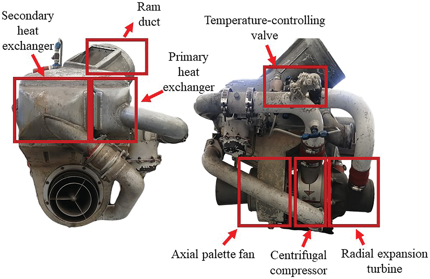
Figure 1: Sabreliner’s ECS main components
The Sabreliner’s ECS consists of an axial palette fan (a), a centrifugal compressor (b) and a radial expansion turbine (c). These three units are mounted on a common shaft, which in the bibliography it is known as ACM [21]. The heat exchanger is a single compact core unit that is divided into two sections to obtain a primary (e) and secondary heat exchanger (d). Approximately one-third of the ram air (ram air refers to the ram air generated by aircraft movement) flows through the section of the primary heat exchanger (HX1) and two-thirds through the section of the secondary heat exchanger (HX2). The heat exchangers are air to air plate-fin cross-flow with rectangular fins.
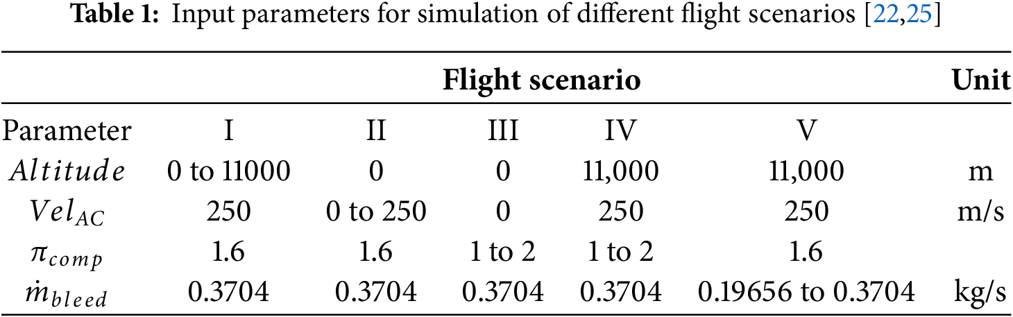
Another important system parameter is the mass flow air rate that feeds the Sabreliner ECS (bleed air), which can vary in a range of 0.19656 to 0.3704 kg/s according to the aircraft manual [22]. This is a very important parameter since it will be the work mass flow to model the ECS.
2.1.1 Description of Air Flow Distribution
In the Sabreliner’s ECS, two fluids are used: the bleed air and the ram air. The first one is the working fluid while the second one is the heat transfer fluid used to cool the ECS’s heat exchangers to reduce the temperature of bleed air. Fig. 2 shows the diagram of the system computed in this paper. Notice that Sabreliner’s ECS (see Fig. 1) takes place from 3 to 7 for bleed air and for ram air from 2 to f.
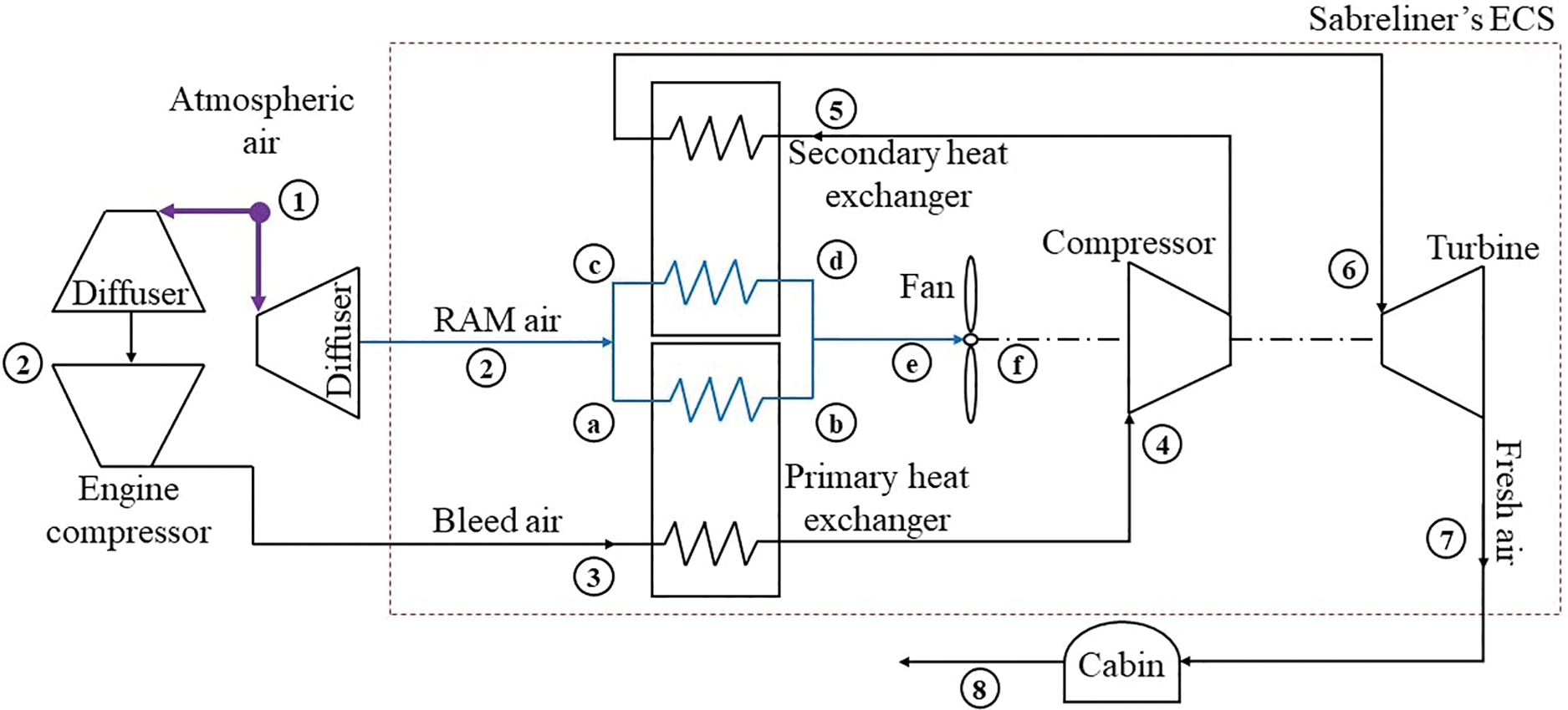
Figure 2: Diagram of the system computed
The diffuser and the compressor are the main components of the aircraft engine which behaviors influence on the ECS efficiency. The atmospheric air (state 1) enters firstly to the diffuser where kinetic energy is converted to flow energy (state 2). After that, air passes through the engine compressor stages where is supposed to achieve the bleed nominal conditions (state 3). At this state, the conditioning work begins: the bleed air passes through the HX1 (state 4) and enters to the compressor where the pressure and temperature rise (state 5). To eliminate the increment of temperature in the compressor, bleed air passes through the HX2 (state 6).
Finally, bleed air crosses an expansion process in the turbine (state 6 to 7) where the pressure and temperature of bleed air decrease drastically. Regularly, bleed air at the turbine output reaches temperatures lower than 273.15 K (state 7), which requires a temperature-controlling valve (g). This valve is responsible for mixing hot air (from HX1) with the cold air that comes from the turbine. In this manner, the output temperature of this mixture is adequate to be injected in the aircraft cabin. Nevertheless, the temperature control valve is not considered because the study focuses especially on the heat exchangers and ACM.
On the other hand, the heat transfer fluid used in the ECS comes from the atmospheric air whose properties such as temperature, pressure and humidity vary all the time. The atmospheric air enters through the diffuser where its pressure and temperature increase depending on the aircraft’s speed. The air flow produced by the aircraft speed is called ram air and also, it can be produced by the ACM fan suction effect. After the diffuser, ram air is conducted to both heat exchangers (HX1 and HX2) through the ram duct (see Fig. 1 or 2 state 2) to cool the bleed air. Upstream both heat exchangers, the ram air enters to the ACM fan and then is expulsed to the ambient.
Is important to mention that in this configuration, the heat exchangers are placed in a parallel position which means, the mass flow rate of air that passes through them is distributed but not equally.
2.1.2 Bleed Air Nominal Conditions
Bleed air is the working fluid that feeds the ECS and is extracted from the compressor engine (see Fig. 2) with constant thermodynamic conditions to ensure the proper functioning of the aircraft engine.
The bleed pressure is regulated to some 250 kPa (from 200 to 300 kPa, depending on the manufacturer); lower values may be insufficient to force the air through the two heat exchangers in the ECS, and higher values may be a waste of resources (the higher the bleed pressure, the higher the cost of fuel).
The bleed temperature is regulated to about 450 K (176.85°C). The air bled from the compressor may be very hot (e.g., at >200°C if compressed from 24 to >250 kPa). Lower temperature values (<450 K) may be insufficient for activate the anti-icing system, and higher values (>450 K) may cause damage to composite structures and plastic materials in the neighborhood of ECS ducts (the ducts are made of heat-resistant fiberglass or aluminum tubes). Notice also that the air conditioning packs are always close to fuel tanks [23,24].
Although the present study is based on a detailed numerical model, future experimental validation using a properly instrumented ECS installation would significantly enhance the reliability and scientific rigor of the results. Such an experimental setup would allow direct comparison between predicted and observed system behavior, thereby confirming the accuracy of the proposed methodology and strengthening its applicability in real-world scenarios.
The methodology used in this study involves analyzing the different phases of the flight mission of the Sabreliner aircraft: take-off, ascent, cruise flight, descent, and landing.
To simulate each flight mission phase, input variables such as bleed mass flow, bleed temperature, bleed pressure, bleed air specific humidity, aircraft speed, flight altitude, and atmospheric parameters (mass flow, temperature, pressure, and specific humidity) are needed to compute the heat exchanger efficiencies. Additionally, the ACM compression ratio and cabin exhaust temperature are required to analyze the work distribution in the ACM and the COP, respectively.
The calculation process is illustrated in Fig. 3, where input and output variables are represented by green and red boxes, respectively. The output variables are determined from the input variables through an iterative procedure based on the energy balance of the ACM system.
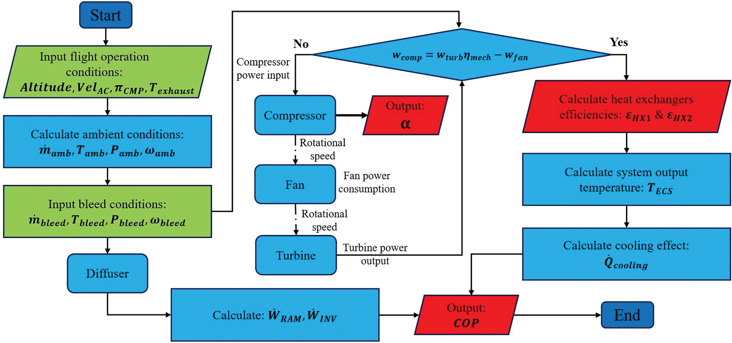
Figure 3: ECS calculation process diagram
The process begins with an initial value of the ACM compressor pressure ratio, which is used to calculate the compressor power input (
The setting of each component in the process diagram (Fig. 3) has been done to facilitate analysis according to the mathematical models developed in the next subsection. In this study, the flight mission phases are addressed by the flight scenarios. The values of altitude, aircraft speed, ACM compression ratio and bleed mass flow for each flight scenario are described in Table 1.
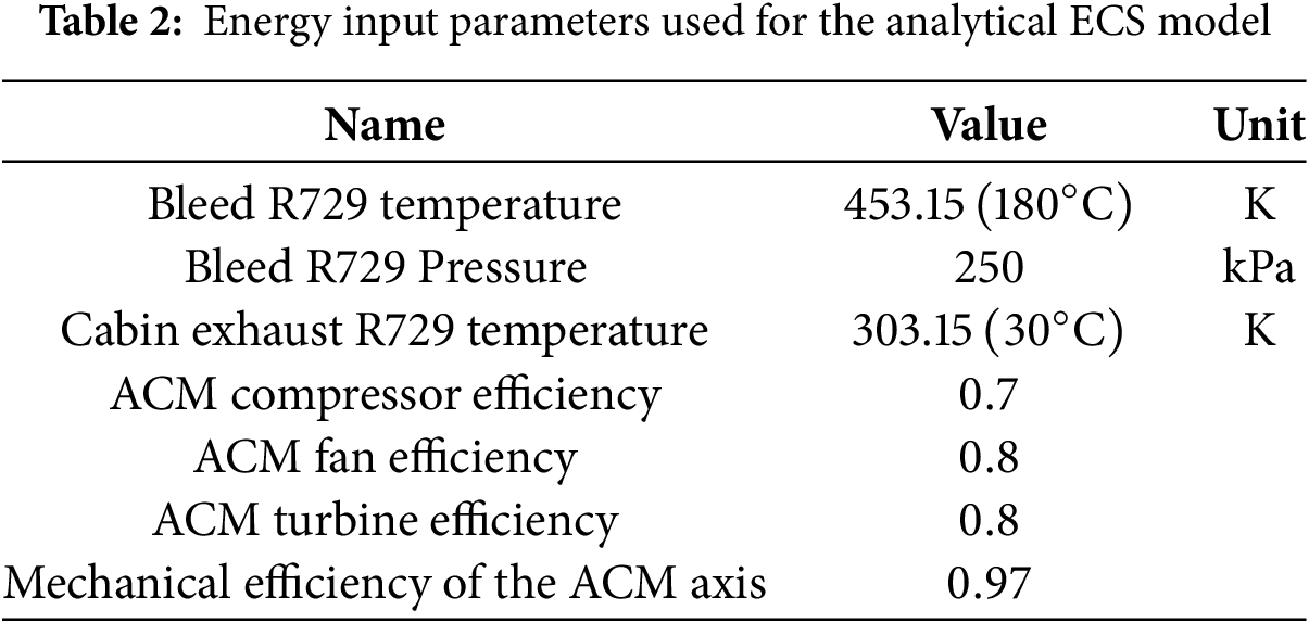
In addition to the input variables described in Table 1, other variables such as bleed air temperature, bleed air pressure, booth outlet temperature, ACM compressor efficiency, ACM turbine efficiency, ACM fan efficiency and ACM mechanical efficiency are needed to calculate the thermal behavior of each ECS component. For our study, the values of these input variables were taken from averaging some acceptable values from [11,12,16,25,26] and they are presented in the Table 2 where it was considered cabin exhaust temperature as constant with a value of 30°C for obtaining all results.
The mathematical model implemented in this study is focused on the heat exchangers, diffuser and ACM (turbine-compressor-fan).
2.3.1 Characterization of the Heat Exchangers
The heat exchanger geometry used in the Sabreliner’s ECS is shown in Fig. 4, where
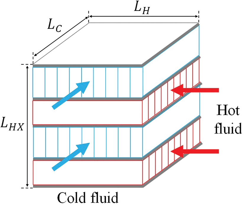
Figure 4: Cross-flow plate-fin heat exchanger structure
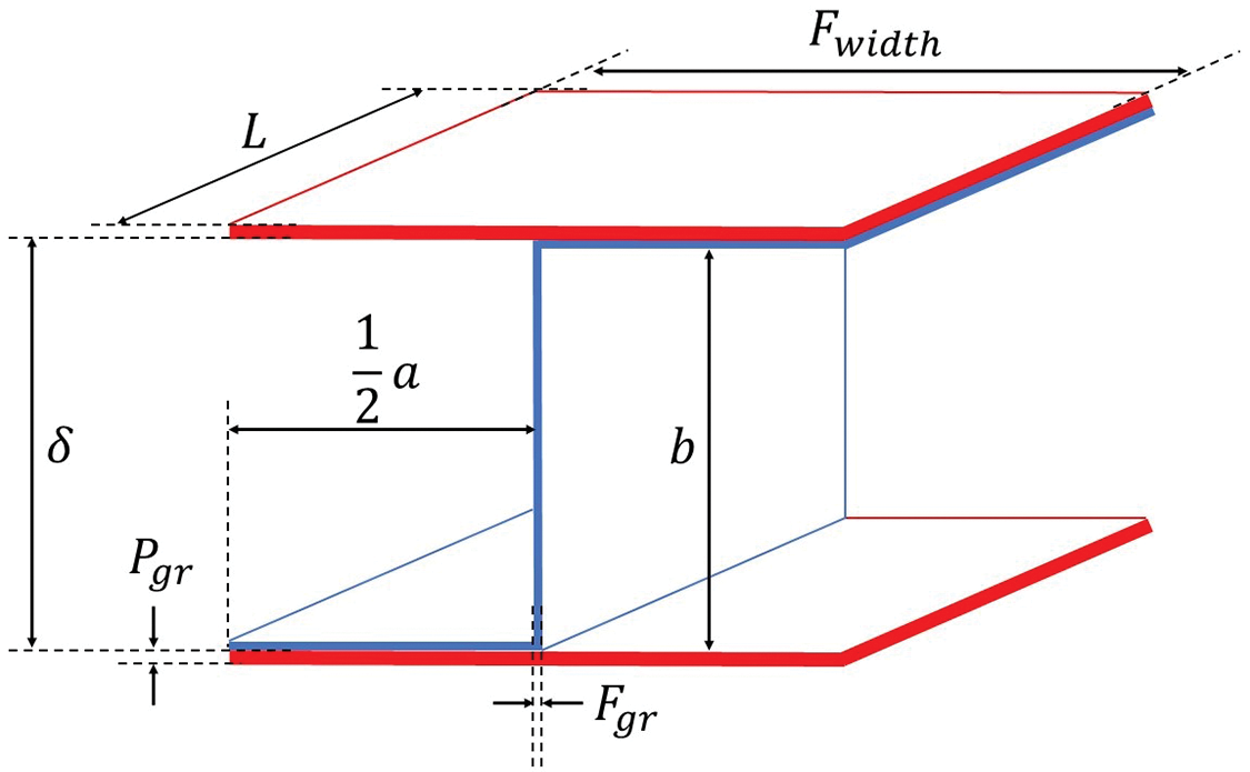
Figure 5: Geometry of rectangular fins of heat exchangers
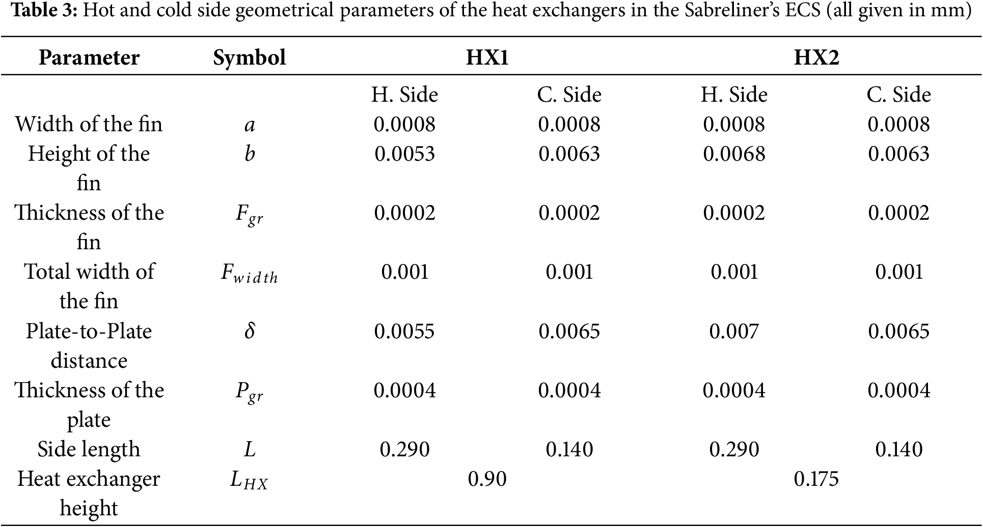
The heat exchanger fin dimensions for the cold and hot sides used in this study are described in Table 3. It is necessary to clarify that the model hereby presented belongs to one side (cold or hot) of a heat exchanger, and can be duplicated to compute the other side. Based on physical parameters described in Table 3, the free flow area and hydraulic diameter of the rectangular fin can be calculated by means of the Eqs. (1) and (2), respectively.
where
The ratio of the secondary surface area to the total surface area for rectangular fins can be calculated as:
In compact heat exchangers, the total heat transfer area per unit volume is larger compared to other technologies; this characteristic is known as areal density,
A heat exchanger channel of this type consists of a hot side plate and a cold side plate joined together (see Fig. 4), so the number of channels that the heat exchanger has is:
The number of fins in a plate on one side of the heat exchanger can be easily calculated as follows:
where
From the definition of the mass velocity it is obtained that:
Now, the Reynolds number for one fin is computed as:
Following the definition of the Prandtl number:
where
Similarly, the Colburn factor for a Reynolds number range of
On the other hand, the definition of the Colburn factor is expressed as:
where the Stanton number
Combining Eqs. (13) and (14) with (10) and solving for
The pressure drop in the heat exchanger is given by:
The total surface temperature effectiveness can be determined from:
where:
The material thermal conductivity of the fin is
where subscripts
Then the total heat transfer areas of each side are calculated as shown below:
Finally, the global heat transfer coefficient of the heat exchanger is computed by means of the following expression:
First, the heat capacities of each side are calculated:
It is necessary to determine which is the minimum
Subsequently, the number of heat exchanger transfer units is calculated:
Finally, the efficiency of the heat exchanger can be obtained [15]:
Once the heat exchanger efficiency was obtained, the actual outlet enthalpy of the heat exchanger can be calculated as:
The properties of the air without humidity can be calculated as an ideal gas. For air with humidity the thermophysical properties (
To initiate the calculation process, it is crucial to establish an atmospheric model that determines the changes in temperature, pressure, and humidity with respect to altitude. The description of this model is provided below.
It can be observed in Fig. 3 that flight altitude and aircraft speed substantially impact the performance of each ECS component. Altitude directly influences the diffuser performance and indirectly affects the heat exchanger efficiencies. Additionally, the power required to generate ram and bleed air mass flows contributes to computing the COP, meaning that atmospheric conditions are the most influential parameters governing the ECS. In this way, the model presented here is based on the ISA (International Standard Atmosphere) [28–30] which defines temperature, pressure and specific humidity as follows:
*This polynomial function was obtained from Linares [31], which is based on ISA.
The altitude (
To determine the temperature and pressure of the ram air at the heat exchangers inlet in the ECS, the diffuser which is located just before the compression stages of the aircraft engine, is analyzed.
When the aircraft is flying, the initial compression of the ambient air is due to the ram effect. The diffuser of the aircraft engine is responsible for producing that effect. Eqs. (33) and (34) describe this process.
The ram power consumption (
where:
The compression ratio in the ACM compressor directly determines ACM operation and indirectly influences the input and output parameters of the two heat exchangers (see Fig. 3). The compression ratio significantly impacts nearly all the input and output conditions of the ECS components. The compression ratio is influenced by the shaft RPMs. It is defined as the ratio between the discharge pressure and the suction pressure within the system. Then the compression ratio is defined as:
where
The actual outlet temperature and the compressor work can be expressed as follows:
The turbine in the ACM plays a vital role as it harnesses air energy from the high-pressure and high-temperature to convert it into mechanical work. This work is used to drive both the compressor and the fan, enabling the continuous circulation of air within the system. As the air expands and undergoes the energy conversion process in the turbine, a substantial drop in temperature occurs, leading to the cooling of the air.
This temperature reduction is of paramount significance as it contributes to the overall cooling and thermal management capabilities of the ACM and, in turn, the ECS. The actual outlet temperature and the turbine work can be expressed as follows:
The actual turbine work is defined as:
The fan in the ACM serves a crucial function by propelling atmospheric air flows towards the heat exchangers. The fan’s continuous operation ensures a constant supply of air, maintaining a steady flow rate through the heat exchangers, and facilitating efficient heat transfer to regulate the temperature and climate inside the aircraft cabin. The actual work consumed for the fan is:
here is important to consider the kinetic energy due to the initial speed of ram air flow (same as the aircraft speed and usually when it is greater than 100 m/s, the terms of kinetic energy should be considered). The actual outlet temperature of the fan is computed as:
where
The shaft serves as a central component that interconnects the turbine, compressor, and fan in the ACM, making them function as an integrated system. As a result, the RPMs of these components are inherently synchronized and operate at the same speed, thus:
The air expansion in the turbine generates the turbine work that is used to compress the air in the compressor and to produce the suction effect in the fan. However, the maximum turbine work that can be transmitted is usually constrained by several losses. The mechanical efficiency (
The speed, work and matching of the three-wheel ACM is achieved through an iterative process which is presented by Tu and Lin [32]. To evaluate the work distribution in the ACM a new parameter is introduced α, this parameter measures the work consumed by the compressor.
This means that the rest of the turbine work is consumed by the fan.
2.3.8 Expression for Calculating the COP
For aircraft ECS, the COP is defined as the ratio of the desired cooling or heating output to the energy input required to achieve that output. For this study, the COP is expressed as:
where
The cooling effect of Sabreliner’s ECS is directly influenced by the temperature difference between the ECS outlet and the cabin exhaust. The greater the temperature difference, the more significant the cooling effect. This direct proportionality means that as the temperature difference increases, the ECS cooling capacity increases as well, it can be easily seen in the next equation:
where
3.1 Validation of the EES Code Designed for the Present Study
The code designed in the Engineering Equation Solver (EES) software for the present study was validated based on the results obtained by Yang and Yang [12] presented in Fig. 6 of their paper published in the literature. The authors modeled five different ECS configurations which are two-wheel simple ACS (2S-ACS), two-wheel bootstrap ACS (2W-ACS), two-wheel bootstrap ACS with high-pressure water separation (2W-ACS-HPWS), three-wheel bootstrap ACS with high-pressure water separation (3W-ACS-HPWS) and four-wheel bootstrap ACS with high-pressure water separation (4WACS-HPWS). Each of these five ECS configurations was analyzed under land conditions (alt = 0 m; Mach = 0) and cruise conditions (alt = 11,000 m; Mach = 0.85) considering HOT atmosphere conditions (
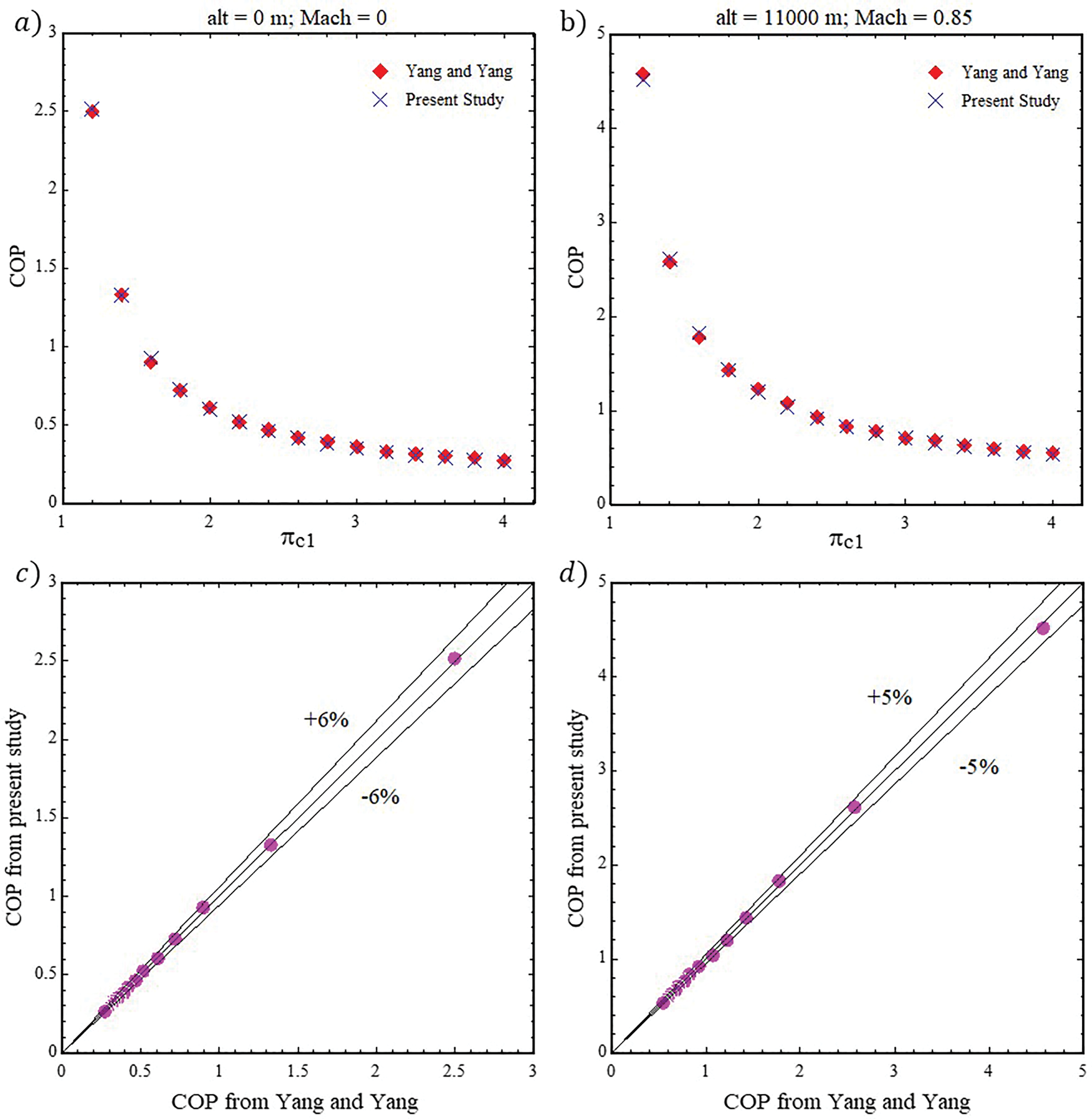
Figure 6: Comparison of results of the present study with those obtained from the work by Yang and Yang [12], (a) Variation of the COP as a function of the engine compressor pressure ratio under land conditions, (b) Variation of the COP as a function of the engine compressor pressure ratio under cruise conditions, (c) Comparison of COP variations under land conditions, (d) Comparison of COP variations under cruise conditions
Among the five ECS configurations studied by Yang and Yang [12], the 3W-ACS-HPWS is similar to the Sabreliner ECS analyzed in the present study. So, based on the results of this configuration, a comparison of results with those obtained in the present study was made as shown in Fig. 6. Fig. 6a,b compares the trends in the engine compressor pressure ratio (
3.2 Effect of Flight Altitude Variations on the ECS Component Performances
This subsection presents the results of flight scenario I (see the first column of Table 1), where the flight altitude varies from 0 to 11,000 m. This scenario allows us to understand the behavior of the heat exchangers and COP in response to variations in flight altitude during the ascent or descent of the Sabreliner.
3.2.1 Heat Exchangers Efficiencies Evaluation Based on Flight Altitude Variations
Under the operating conditions presented in the first column of Table 1, the efficiencies of both primary and secondary heat exchangers were evaluated using the mathematical models developed in Section 2.3.1. The behavior of the efficiency of the two heat exchangers when the Sabreliner faces variations in altitude from 0 to 11,000 m is depicted in Fig. 7, specifically on the right side of the graph.
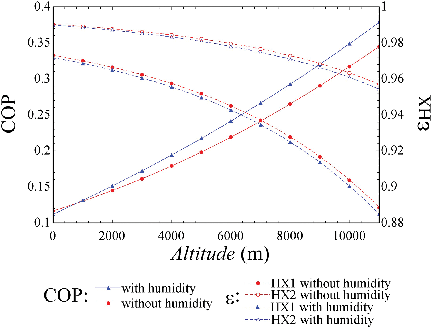
Figure 7: Variation of COP and heat exchanger efficiencies with respect to the flight altitude of the aircraft
It can be seen that the efficiencies of both heat exchangers decrease as flight altitude increases. The density of the heat transfer fluid (ram air) is the property that most affects these efficiencies because it decreases as flight altitude increases. Consequently, the mass flow of the heat transfer fluid decreases, causing a reduction in the ram air heat capacity (
Based on Eq. (28), it can be understood that the increase in
However, the first heat exchanger (HX1) is more impacted since, in the ECS, the size of HX1 is half that of the second heat exchanger (HX2), meaning that the total heat transfer areas (
3.2.2 COP Evaluation Based on Flight Altitude Variations
The behavior of the ECS COP when the Sabreliner experiences altitude variations from 0 to 11,000 m is described in Fig. 7, specifically on the left side of the graph. Generally, the COP increases as the Sabreliner’s flight altitude increases. This is a consequence of atmospheric air temperature variations, which can decrease from 288.15 to 216.8 K during takeoff as altitude increases from 0 to 11,000 m. Consequently, the heat transfer fluid temperature decreases, improving heat dissipation in the bleed air and subsequently reduces the fresh air temperature at the ECS outlet (
It is important to note that, despite this trend, a significant increase in COP is not observed despite the substantial change in the heat transfer fluid temperature, rising from 0.11 to a maximum value of 0.38 at cruising altitude. This is due to two factors involved in the COP calculation:
On the other hand, increasing altitude leads to an increase in
Regarding the impact of humidity on air, it can be observed that the curves initially differ by approximately 4.11%, reaching a final difference of 9.28% at 11,000 m between both fluids. Additionally, there is a noticeable altitude range where the COP of air with humidity is lower. This implies that there is a point of intersection between the two curves, occurring at approximately 850 m. Beyond this point, the COP of air with humidity becomes higher than that of air without humidity.
At this altitude, the humidity in the ram air does not evaporate during the cooling process of the heat exchangers, thus maintaining the humidity in a liquid state throughout the heat exchange process. Consequently, a COP increase results for the case of air with humidity, as liquid water possesses superior heat dissipation properties compared to water vapor. This is notably evident in the significant difference between the specific heat of water in its liquid and gaseous states, with the specific heat being higher in the liquid state than in the gas state.
3.3 Effect of Aircraft Speed Variations on the ECS Component Performances
This subsection describes the behavior of heat exchangers and COP when facing aircraft speed variations from 0 to 250 m/s during the taxiing of the Sabreliner aircraft as described in flight scenario II (see Table 1).
3.3.1 Heat Exchangers Efficiencies Evaluation Based on Aircraft Speed Variations
Fig. 8 shows the efficiency behavior of the ECS heat exchangers due to the variation in aircraft speed. Significant negative slopes can be observed in the efficiency of both ECS heat exchangers when the aircraft speed varies from 0 to 18 m/s for HX2 and from 0 to 35 m/s for HX1.
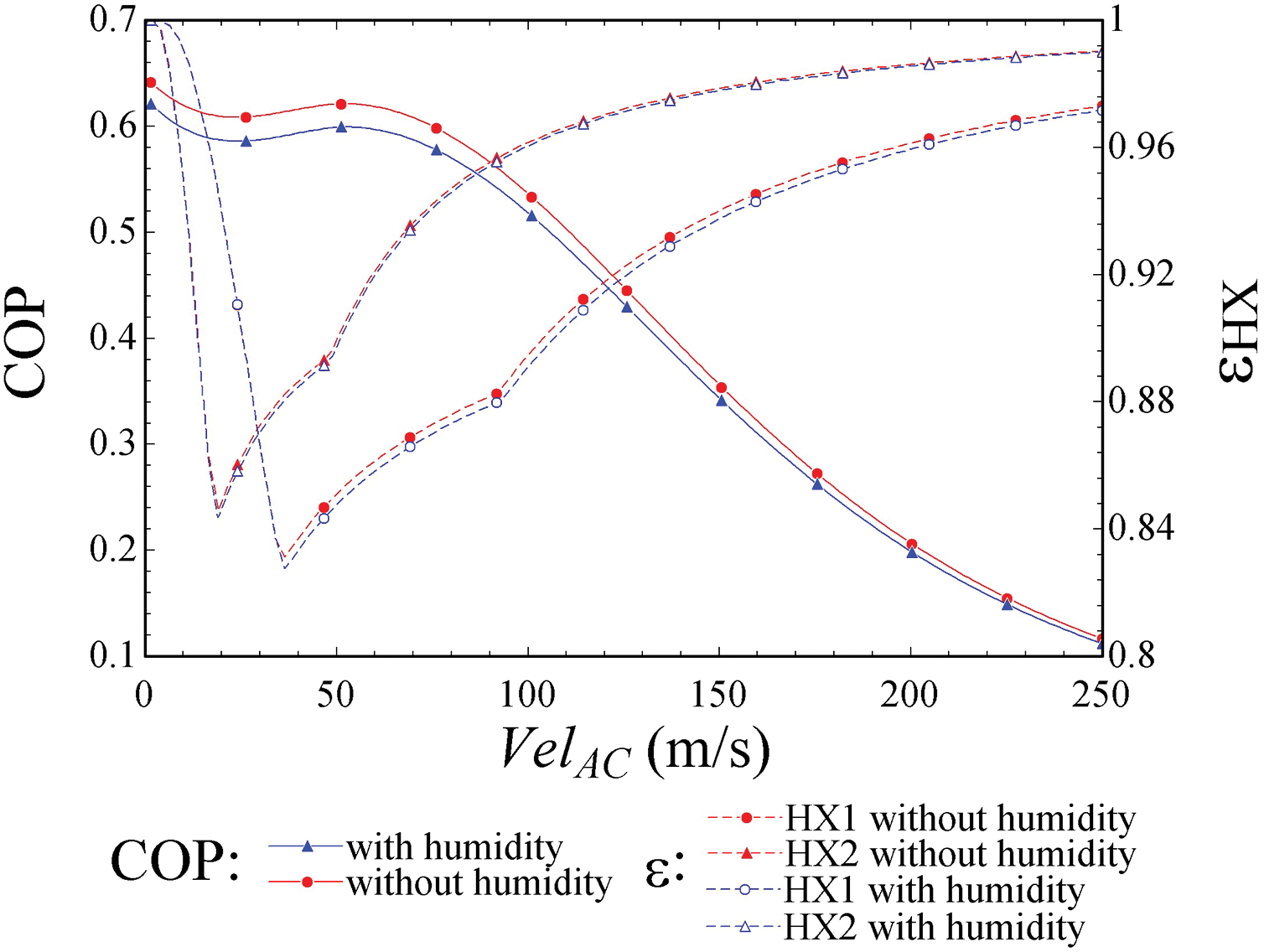
Figure 8: Variation of COP and heat exchanger efficiencies with respect to the aircraft speed on land
This behavior is due to the low ram air mass flow produced by the aircraft’s low speeds, starting from 0 m/s and increasing until 250 m/s. This causes that
This happens until the ram air mass flow reaches the constant value of the bleed air mass flow (
Moreover, it is evident that the efficiency of HX1 is significantly more influenced by the aircraft’s speed compared to that of HX2. This is because HX2 efficiency depends on the performance of HX1, with several output parameters from HX1 serving as inputs for HX2. This relationship explains the similar behavior observed in both efficiency curves.
On the other hand, it is noticeable that the negative impact of humidity is more pronounced around the inflection point of the curve, showing a difference of 0.38% and 0.26% for HX1 and HX2, respectively. Towards the higher end of the curve, this effect diminishes, reducing to minimal levels of 0.14% for HX1 and 0.04% for HX2. This phenomenon is attributed to the ram effect, which increases the temperature and pressure of humid air, thereby aligning its properties more closely with dry air, as previously mentioned.
3.3.2 COP Evaluation Based on Aircraft Speed Variations
Fig. 8 illustrates how the COP of the ECS responds to changes in aircraft speed. Initially, a slight decline in COP is observed when the speed ranges from 0 to approximately 30 m/s. This decline directly correlates with the decrease in heat exchanger efficiencies discussed in the previous subsection. As the efficiencies of the heat exchangers decrease, so does the COP. Subsequently, a small increase in COP is noted, similarly linked to the behavior of the heat exchanger efficiencies. Beyond the earlier mentioned speed range, these efficiencies begin to rise, contributing to a slight increase in COP. This relationship is captured in Eq. (52), where a decrease in the temperature at the ECS output (
However, as aircraft speed further increases, the COP decreases, consistent with findings from previous studies such as those by Conceição et al. [8] and Alvarenga et al. [11]. This decline at higher speeds is directly attributed to the power required to generate ram air mass flow and the associated drag effects, evaluated by Eq. (35). While increasing ram air mass flow can marginally improve COP, the primary impact on COP stems from the power consumption associated with moving large volumes of air through the heat exchangers.
It is noteworthy that the final COP value at a speed of 250 m/s in Fig. 8 aligns with the initial COP value corresponding to sea level altitude in Fig. 7. In another scenario, the gap between the two humidity curves diminishes from 3.26% at 0 m/s to almost negligible levels as speed increases. This convergence indicates that air with humidity approaches the behavior of dry air as its pressure and temperature rise.
3.3.3 ACM Work Distribution Evaluation Based on Aircraft Speed Variations
An important internal output parameter to analyze is the percentage of work consumed by the ACM compressor (
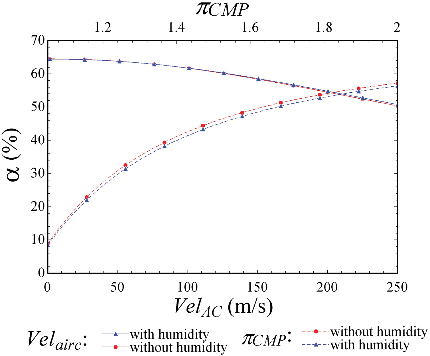
Figure 9: Behavior of the ACM work distribution facing the aircraft speed and ACM compressor ratio variation, on land
It is observed in Fig. 9 that the work consumed by the ACM compressor decreases as the aircraft speed increases, causing the α to decrease. This is because both the ACM compressor and fan are powered by the ACM gas turbine, whose power remains constant (see Eq. (48)). However, as the aircraft speed increases, the ram air mass flow rate also increases, causing a grow in the work required by the fan, and consequently, the compressor's efficiency is affected, causing a decrease in α.
Additionally, it is observed that the maximum work consumption by the compressor, approximately 64.4%, occurs when the aircraft is stationary, while the minimum, around 50%, is reached at a speed of 250 m/s. In another scenario, humidity in the air causes approximately 0.1% less work consumption by the ACM compressor in the speed range of 0 to 80 m/s. Beyond this range, dry air consumes approximately 0.81% less work.
3.4 Effect of the ACM Compression Ratio Variations on the ECS Component Performances
The ACM compression ratio (
The compression ratio is analyzed to provide a comprehensive understanding of the system’s response to variations in ACM rotational speed during real flight scenarios. Subsequent sections will evaluate ECS output parameters under both ground and cruise conditions, focusing on changes in the ACM compression ratio.
3.4.1 ACM Work Distribution Evaluation Based on ACM Compression Ratio Variations
Static Aircraft on Land
The analysis is based on the third scenario outlined in Table 1. In this scenario, there is no variation in ACM work distribution relative to the compression ratio of the ACM compressor. This is because, when the aircraft is stationary on the ground, there is no ram air mass flow (
Aircraft Flying at Altitude and Cruise Speed
This flight phase corresponds to the fourth scenario described in Table 1. Fig. 9 illustrates a parabolic trend in the percentage of work consumed by the ACM compressor under these conditions. Unlike the stationary scenario, there is variation in the work distribution along the shaft during flight. This variation can be attributed to the presence of ram air mass flow entering the fan with an initial induced speed (
3.4.2 COP Evaluation Based on ACM Compression Ratio Variations
Static Aircraft on Land
The behavior of the COP in relation to variations in the ACM compression ratio when the aircraft is stationary on land is depicted in Fig. 10. The COP increases proportionally with an increase in the ACM’s compression ratio. This relationship is directly influenced by the enthalpy drop in the ACM turbine.
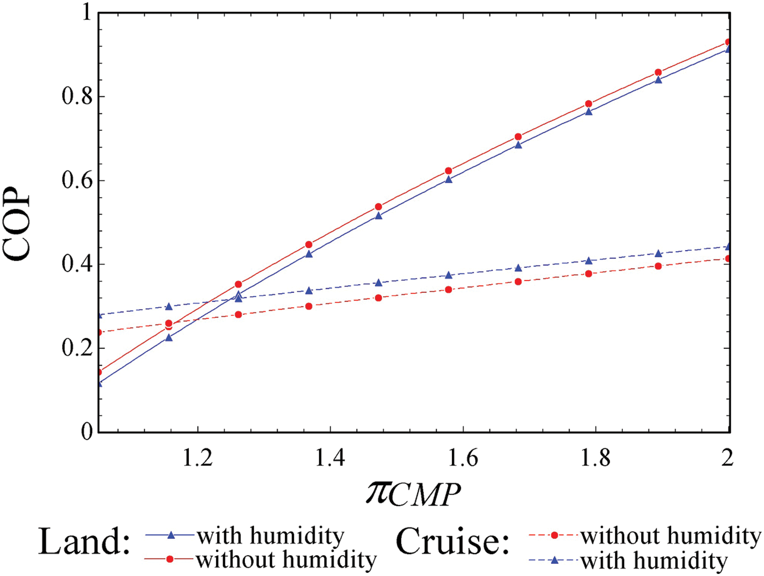
Figure 10: Variation of COP with respect to the ACM compression ratio, on land and cruise
As the compressor requires more power to compress the air, the enthalpy drop in the turbine increases, resulting in a significant decrease in the temperature at the turbine’s outlet (
The analysis shows that the highest COP value achieved is associated with an ACM compression ratio of approximately 2, yielding a COP of around 0.93. This finding is consistent with Yang and Yang [12], affirming that the ACM compression ratio is the parameter exerting the most significant influence on COP.
Regarding the impact of humidity, it is evident that dry air achieves approximately 11.21% higher COP values compared to humid conditions. This result aligns with previous studies which have consistently shown that increased humidity during the compression process reduces compression work and, consequently, lowers the COP [19,33–35].
Aircraft Flying at Altitude and Cruise Speed
Fig. 10 also depicts the COP behavior of the ECS during cruising conditions. A similar trend to that observed on land can be seen, albeit with smaller COP values. The decrease in COP during cruise flights can be primarily attributed to two main factors. Firstly, the power consumption of the aircraft engines to produce the ram air mass flow at cruise speed, along with its associated drag effect. Secondly, the energy required to compress the atmospheric air conditions (as per Eqs. (30) and (31)) to the pressure level needed by the ECS (refer to Table 2). These combined effects negatively impact the COP, resulting in its reduced scale during cruise operations.
In contrast, when the aircraft is stationary, there is no energy consumption due to drag from flowing atmospheric air. In this scenario, the ram air mass flow is solely due to the fan suction effect and is unaffected by the aircraft’s motion, thereby eliminating associated energy costs.
It is also noteworthy that despite the lower temperatures of ram air at cruise altitude, which enhances cooling efficiency compared to ground conditions, the COP is significantly affected by the energy consumed in the aforementioned factors.
An important observation in this context is that humidity has a positive impact on COP compared to ground conditions. Specifically, humid air shows an increase of approximately 10.46% in COP compared to dry conditions.
3.5 Effect of the Bleed Air Mass Flow Variations on the ECS Component Performances
The analysis is centered on the fifth scenario described in Table 1, detailing the behaviors of the heat exchanger efficiencies, ECS COP, and ACM work distribution for the Sabreliner aircraft at cruising altitude and speed, considering variations in the ACM’s bleed air mass flow.
3.5.1 Heat Exchangers Efficiencies Evaluation Based on Bleed Air Mass Flow Variations
Fig. 11 illustrates the behavior of the heat exchanger efficiencies in response to variations in the bleed air mass flow during cruising conditions. The results indicate that increasing the bleed air mass flow leads to a decrease in the efficiencies of both heat exchangers. This trend arises because a higher bleed air mass flow corresponds to a larger thermal load that needs to be dissipated, directly reducing the heat exchanger efficiencies.
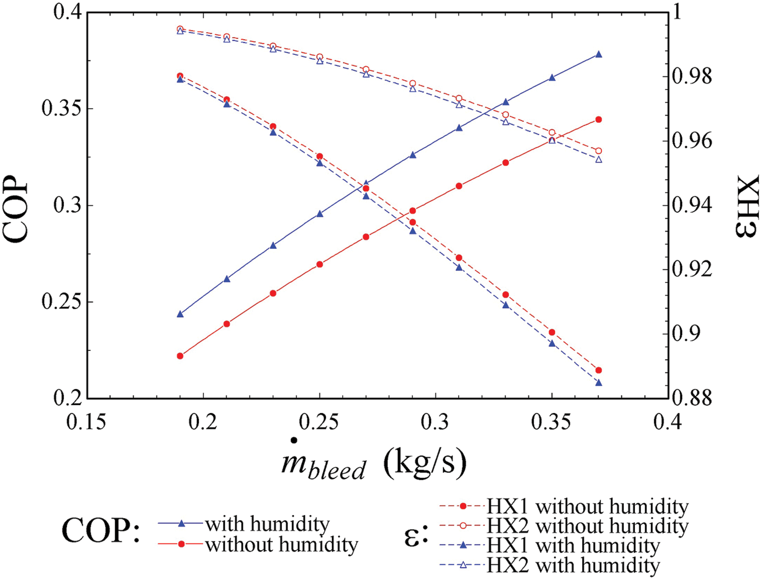
Figure 11: Behavior of COP and heat exchanger efficiencies facing the bleed air mass flow variation, on cruise
Mathematically, this effect can be understood by the increase in the effectiveness factor,
The first heat exchanger is particularly more affected because it initially receives and dissipates the greatest thermal load. In contrast, the second heat exchanger benefits from pre-cooling by the first heat exchanger and its larger size, which enhances its cooling capacity and mitigates the impact on its efficiency.
Furthermore, the observed behavior parallels as that shown in Fig. 7, where variations in flight altitude were examined. This similarity arises because the ram air flow is directly influenced by flight altitude. Similarly, in this case, varying the bleed air flow directly affects the efficiencies of the heat exchangers on the hot side.
Regarding humidity, dry air shows an efficiency increase of approximately 0.27% in HX1 and 0.28% in HX2 compared to humid conditions.
3.5.2 COP Evaluation Based on Bleed Air Mass Flow Variations
Fig. 11 depicts the COP behavior as a function of bleed air mass flow, showing a direct proportional relationship. As observed, COP increases with higher bleed air mass flow. This increase is primarily attributed to the corresponding increase in cooling effect (as per Eq. (52)), resulting in an enhancement of COP (Eq. (50)).
It is important to note, that increasing bleed air mass flow also escalates power consumption by the aircraft’s engines and decreases the efficiencies of the heat exchangers. These factors contribute to only slight positive changes in COP despite the increased cooling effect. Regarding the influence of humidity, the COP is observed to be 9.29% higher when using humid air. This finding corroborates earlier observations that water content in air reduces compression work. Furthermore, humid air contributes to a higher COP due to its higher specific heat compared to dry air. However, continuous humidity introduction into the cabin can lead to undesirable corrosion on surfaces. To mitigate this issue, aircraft cabins are maintained at very low humidity levels [24].
3.5.3 ACM Work Distribution Evaluation Based on Bleed Air Mass Flow Variations
Fig. 12 illustrates the behavior of the ACM compressor work consumption. There is minimal variation in consumption, approximately 0.02%, which is expected due to the ECS operating with separate streams—one for bleed air and another for ram air. As a result, changes in bleed air mass flow do not significantly impact fan work consumption, as it remains independent of the bleed air mass flow.
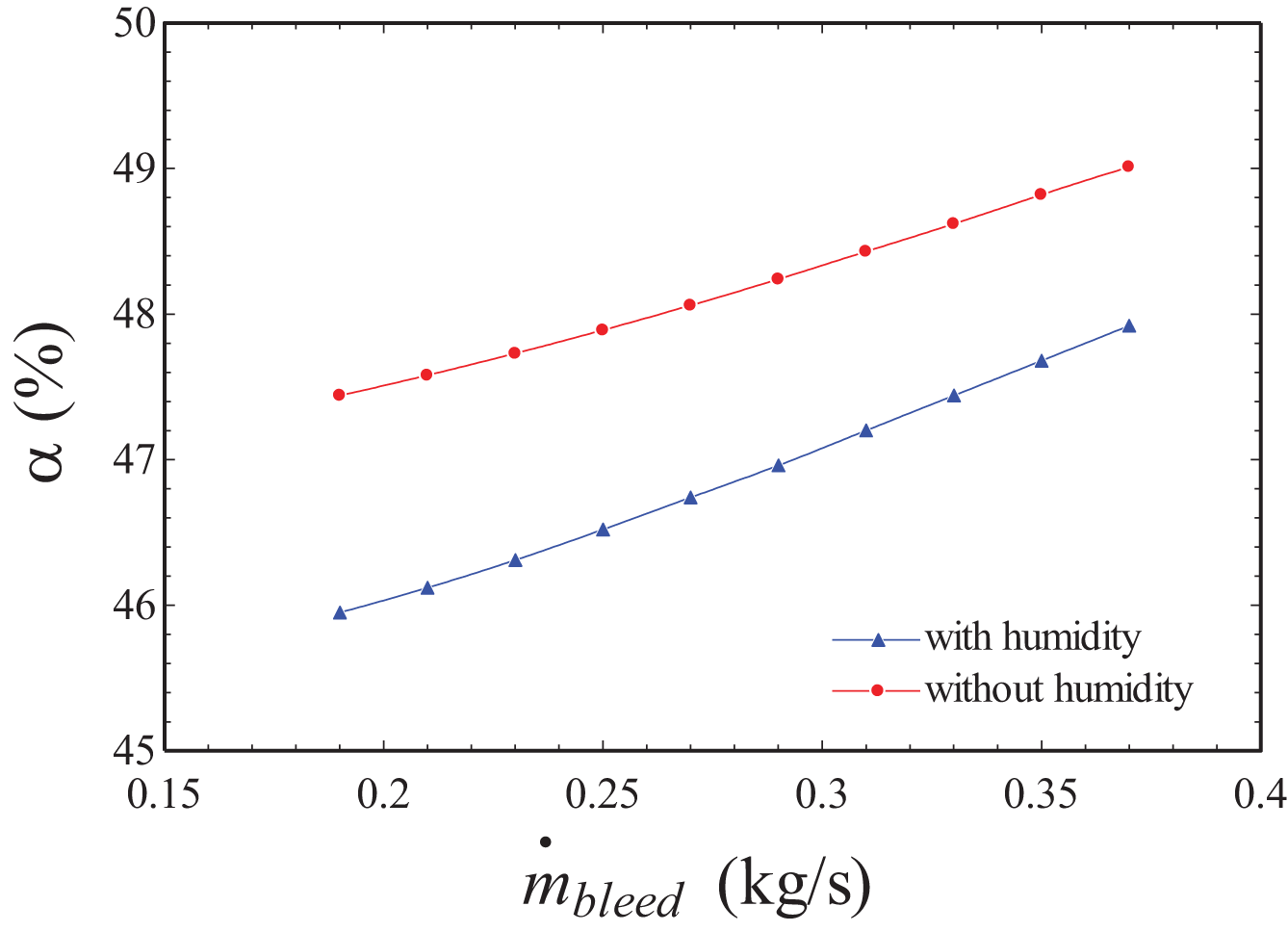
Figure 12: Behavior of the ACM work distribution facing the bleed air mass flow variation, on cruise
Regarding humidity, as anticipated, air with humidity consumes approximately 2.72% less work during the compression process, consistent with previous explanations.
This paper analyzed the effects of flight altitude, aircraft speed, ACM compression ratio, and bleed air mass flow variations on the performance of ECS components, with a particular emphasis on considering the influence of atmospheric humidity. To conduct this analysis, a methodology was developed to compute key output variables.
Heat exchanger efficiencies were computed based on the physical dimensions of the heat exchangers to better understand the parameters that influence them.
The results obtained under various flight scenarios are summarized as follows:
• The COP exhibited varying behaviors under different flight scenarios, with humidity in the air showing an average percentage difference of 7.9% compared to dry air conditions.
• The efficiency of heat exchangers showed an average percentage difference of 0.22% in behavior between humid and dry air conditions.
• In terms of ACM work distribution, humidity conditions resulted in consuming approximately 2.91% less work from the turbine compared to dry air.
The COP was found to increase with altitude, ACM compression ratio, and bleed air mass flow, while it decreased with increasing aircraft velocity. Aircraft speed was identified as the primary external factor significantly impacting COP due to the energy required to create ram air flow
Internally, the ACM compression ratio was identified as the key parameter influencing COP, with significant improvements observed under land conditions as the ACM compression ratio varied. Efficiency of heat exchangers was primarily influenced by the mass flows of both bleed air and ram air, along with the Reynolds number. Higher aircraft speeds positively impacted heat exchanger efficiencies, whereas increases in altitude and bleed air mass flow decreased efficiencies, particularly affecting the secondary heat exchanger more than the primary.
The work consumed by the ACM compressor showed a decrease with increasing aircraft velocity and an increase with higher ACM compression ratio and bleed air mass flow. Flight altitude variations did not significantly affect ACM work distribution.
So that, under both ground and cruise conditions, variations in ACM compression ratio did not affect heat exchanger efficiencies, while variations in bleed air mass flow during ground conditions did not influence the evaluated output parameters.
This work has provided a general overview of ECS performance under the various operating conditions encountered by aircraft in a typical flight mission. It serves as a tool for aeronautical engineers that easily identifies points of low ECS performance, revealing their possible causes. Various parameters were compared under varying operating conditions to determine which parameter has the greatest influence on the ECS and to uncover the causes.
This work seeks to encourage designers to propose solutions to these explored improvement points. It is also worth mentioning that this opens a field of research to find those balance points where improving the performance of one parameter does not significantly affect the impact of another parameter on system performance.
As seen, the COP of this type of system is very low due to its high energy consumption. It’s also important to note that some operating conditions in an aircraft are difficult to avoid; however, it’s possible to propose new technologies for critical ECS components that reduce high energy consumption or even change the operating paradigm and migrate it to other types of ECS proposals.
Acknowledgement: Not applicable.
Funding Statement: The authors received no specific funding for this study.
Author Contributions: The authors confirm contribution to the paper as follows: formal analysis, investigation and writing: J. E. López-Gil; original draft preparation: J. F. Ituna-Yudonago, J. E. López-Gil; project administration, software, writing—review & editing: J. F. Ituna-Yudonago, V. Pérez-García; conceptualization and validation: V. Martínez-Calzada, J. L. Rodríguez-Muñoz; resources and supervision: J. L. Rodríguez-Muñoz, J. F. Ituna-Yudonago; visualization and methodology: J. Serrano-Arellano. All authors reviewed the results and approved the final version of the manuscript.
Availability of Data and Materials: Not applicable.
Ethics Approval: Not applicable.
Conflicts of Interest: The authors declare no conflicts of interest to report regarding the present study.
Glossary
Nomenclature
| Width of the fin | ||
| Area | ||
| Altitude | ||
| Total heat transfer area | ||
| Free flow area of the fin | ||
| Height of the fin | ||
| Sound velocity | ||
| Heat capacity | ||
| Specific heat at constant pressure | ||
| Ratio of heat capacities | – | |
| Diameter | ||
| Hydraulic diameter | ||
| Friction factor | – | |
| Total width of the fin | ||
| Thickness of the fin | ||
| Ratio of the secondary surface area to the total surface area | – | |
| Mass velocity | ||
| Convective heat transfer coefficient | ||
| h | Enthalpy | |
| Colburn factor | – | |
| Thermal conductivity | ||
| Length | ||
| Mach number | – | |
| Mass flow | ||
| Number of channels | – | |
| Total number of fins on one side | – | |
| Number of heat exchanger transfer unit | – | |
| Pressure | ||
| Prandtl number | – | |
| Thickness of the plate | ||
| Wetted perimeter | ||
| Cooling Effect | ||
| Universal gas constant | ||
| Reynolds number | – | |
| Stanton number | – | |
| Temperature | ||
| Environmental control system output temperature | ||
| Cabin exhaust temperature | ||
| Rotacional speed | ||
| Global heat transfer coefficient | ||
| Velocity | ||
| Total volume of the unit | ||
| Specific work | ||
| Power used to produce mass flow of bleed air | ||
| Power used to produce mass flow of ram air | ||
| Abbreviations | ||
| ACM | Air Cycle Machine | |
| ACS | Air Cycle System | |
| CMP | Centrifugal compressor | |
| COP | Coefficient of Performance | |
| DIF | Diffuser | |
| ECS | Environmental Control System | |
| FAN | Axial palette fan | |
| HPWS | High-Pressure Water Separation | |
| HX | Heat Exchanger | |
| ISA | International Standard Atmosphere | |
| PID | Proportional-Integral-Derivative | |
| ram | Airflow created by a moving object | |
| RPMs | Revolutions per minute | |
| TRB | Radial expansion turbine | |
| VCM | Vapor Cycle Machine | |
| Greek Symbols | ||
| Percentage of turbine work consumed by the compressor: | % | |
| Area density | ||
| Plate-to-Plate distance | ||
| Pressure drop | ||
| Heat exchanger efficiency | – | |
| Efficiency | – | |
| Total surface temperature effectiveness | – | |
| Compression ratio | – | |
| Engine compression ratio | – | |
| Ratio of the surface area of one side to the total volume of the unit | ||
| Density | ||
| Viscosity | ||
| Ratio of specific heats | – | |
| Specific humidity | ||
| Subscripts | ||
| Atmospheric air | ||
| Aircraft | ||
| Bleed air | ||
| Cold side | ||
| Compressor | ||
| Fan | ||
| Rectangular fin | ||
| Hot side | ||
| Primary heat exchanger | ||
| Secondary heat exchanger | ||
| Maximum | ||
| Mechanical | ||
| Minimum | ||
| Input parameter | ||
| Output parameter | ||
| After ram effect | ||
| Turbine | ||
References
1. MIL-STD-210. The US department of defense non-standard atmospheres [Internet]. Washington, DC, USA: U.S Department of Defense; 2021 [cited 2025 Aug 1]. Available from: https://www.pdas.com/milstd210.html. [Google Scholar]
2. Dechow M, Nurcombe C. Aircraft environmental control systems. In: Air quality in airplane cabins and similar enclosed spaces. Berlin/Heidelberg, Germany: Springer; 2005. p. 3–24. doi:10.1007/b107234. [Google Scholar] [CrossRef]
3. SAE ARP147D. Environmental control systems terminology. Warrendale, PA, USA: SAE; 2001. doi:10.4271/arp147d. [Google Scholar] [CrossRef]
4. Yang H, Yang C, Zhang X, Yuan X. Influences of different architectures on the thermodynamic performance and network structure of aircraft environmental control system. Entropy. 2021;23(7):855. doi:10.3390/e23070855. [Google Scholar] [PubMed] [CrossRef]
5. SAE AIR 1168/3. Aerothermodynamic systems engineering and design. Warrendale, PA, USA: SAE; 2004. doi:10.4271/air1168/3. [Google Scholar] [CrossRef]
6. Santos APP, Andrade CR, Zaparoli EL. A thermodynamic study of air cycle machine for aeronautical applications. Int J Thermo. 2014;17(3):117. doi:10.5541/ijot.538. [Google Scholar] [CrossRef]
7. Garrett DF. Aircraft systems and components. Englewood, CO, USA: Jeppesen Sanderson; 1992. [Google Scholar]
8. Conceição ST, Zaparoli EL, Turcio WHL. Thermodynamic study of aircraft air conditioning air cycle machine: 3-wheel × 4-wheel. Warrendale, PA, USA: SAE International; 2007. Report No.: 2007-01-2579. doi:10.4271/2007-01-2579. [Google Scholar] [CrossRef]
9. Yang H, Yang C. Thermodynamic characteristics and order degree of air cycle system. Int J Refrig. 2020;118(4):61–71. doi:10.1016/j.ijrefrig.2020.03.027. [Google Scholar] [CrossRef]
10. Jennions I, Ali F, Miguez ME, Escobar IC. Simulation of an aircraft environmental control system. Appl Therm Eng. 2020;172(6):114925. doi:10.1016/j.applthermaleng.2020.114925. [Google Scholar] [CrossRef]
11. Alvarenga MA, Andrade CR, Zaparoli EL. A thermodynamic analysis of three and four-wheel air cycle machines for aeronautical applications. Int Rev Mech Eng IREME. 2015;9(2):190. doi:10.15866/ireme.v9i2.5543. [Google Scholar] [CrossRef]
12. Yang H, Yang C. Derivation and comparison of thermodynamic characteristics of endoreversible aircraft environmental control systems. Appl Therm Eng. 2020;180(4):115811. doi:10.1016/j.applthermaleng.2020.115811. [Google Scholar] [CrossRef]
13. Yang H, Yang C. Application of scaling-endoreversible thermodynamic analysis model to aircraft environmental control system-methodology development. Int J Refrig. 2020;112(4):90–9. doi:10.1016/j.ijrefrig.2019.12.006. [Google Scholar] [CrossRef]
14. Zhao H, Hou Y, Zhu Y, Chen L, Chen S. Experimental study on the performance of an aircraft environmental control system. Appl Therm Eng. 2009;29(16):3284–8. doi:10.1016/j.applthermaleng.2009.05.002. [Google Scholar] [CrossRef]
15. Liu Q, Zhuang L, Wen J, Dong B, Liu Z. Thermodynamic optimization of aircraft environmental control system using modified genetic algorithm. Processes. 2022;10(4):721. doi:10.3390/pr10040721. [Google Scholar] [CrossRef]
16. Yang H, Zhang X, Wang C, Yang C. Experimental and theoretical study on a novel energy-saving ECS for commercial airliners. Appl Therm Eng. 2017;127:1372–81. doi:10.1016/j.applthermaleng.2017.08.043. [Google Scholar] [CrossRef]
17. Che L, Zhang XJ, Yang C. A new concept environmental control system with energy recovery considerations for commercial aircraft. In: Proceedings of the 44th International Conference on Environmental Systems; 2014 Jul 13–17; Tucson, AZ, USA. [Google Scholar]
18. Negi VPS, Ranganayakulu C. Thermal performance of three-wheel and split-wheel air cycle systems for a civil aircraft environmental control system (ECS). Int J Refrig. 2024;166:196–211. doi:10.1016/j.ijrefrig.2024.06.021. [Google Scholar] [CrossRef]
19. Chen L, Zhang X, Wang C, Yang C. A novel environmental control system facilitating humidification for commercial aircraft. Build Environ. 2017;126(12):34–41. doi:10.1016/j.buildenv.2017.09.013. [Google Scholar] [CrossRef]
20. Childs TG, Jones AB, Chen R, Murray A. A study into refrigeration cycle working fluids using an air cycle machine environmental control system. In: 54th AIAA Aerospace Sciences Meeting; 2016 Jan 4–8. San Diego, CA, USA. 2190 p. doi:10.2514/6.2016-2190. [Google Scholar] [CrossRef]
21. Merzvinskas M, Bringhenti C, Tomita JT, de Andrade CR. Air conditioning systems for aeronautical applications: a review. Aeronaut J. 2020;124(1274):499–532. doi:10.1017/aer.2019.159. [Google Scholar] [CrossRef]
22. Sabreliner Initial Study Guide (265–65) [Internet]. Columbus, OH, USA: Flight Safety International; 1982 [cited 2025 Aug 1]. Available from: https://www.google.com.mx/books/edition/Sabreliner_Initial_Study_Guide_265_65/DBtnGwAACAAJ?hl=es. [Google Scholar]
23. Shao L, Tan J, Liu W, Yang J, Hei B, Qu J. System performance comparison of oxygen consumption and air separation for aircraft fuel tank inerting. Case Stud Therm Eng. 2024;60:104749. doi:10.1016/j.csite.2024.104749. [Google Scholar] [CrossRef]
24. Martinez I. Aircraft environmental control (1995–2013) [Internet]. [cited 2025 Aug 1]. Available from: http://imartinez.etsiae.upm.es/tc3/Aircraft%20ECS.pdf. [Google Scholar]
25. Meng F, Sun J, Zhou Y, Gao Z, Cheng D. Modeling and validating of air cycle machine in aircraft environmental control system. Huagong Xuebao/CIESC J. 2020;71:328–34. doi:10.11949/0438-1157.20191125. [Google Scholar] [CrossRef]
26. Li X, Chen Q, Hao JH, Chen X, He KL. Heat current method for analysis and optimization of a refrigeration system for aircraft environmental control system. Int J Refrig. 2019;106:163–80. doi:10.1016/j.ijrefrig.2019.06.004. [Google Scholar] [CrossRef]
27. García-Castillo J, Picón-Núñez M. Physical dimensions as a design objective in heat transfer equipment: the case of plate and fin heat exchangers. Energies. 2021;14(8):2318. doi:10.3390/en14082318. [Google Scholar] [CrossRef]
28. Pollock RD, Hodkinson PD. The earth’s atmosphere: ernsting’s aviation and space medicine. Boca Raton, FL, USA: CRC Press; 2025. p. 3–13. [Google Scholar]
29. Kurzke J, Halliwell I, Hill R. Gas properties and standard atmosphere. In: Propulsion and power. Cham, Switzerland: Springer Nature; 2025. p. 775–80. doi:10.1007/978-3-031-65026-0_20. [Google Scholar] [CrossRef]
30. Movahedian A, Marinaro G, Frosina E. A fast-time MATLAB model of an aeronautical low-temperature PEM fuel cell for sustainable propulsion and compressor behavior at varying altitudes. Sustainability. 2025;17(13):5817. doi:10.3390/su17135817. [Google Scholar] [CrossRef]
31. Linares DP. Modeling and simulation of an aircraft environmental control system. Montréal, QC, Canada: Ecole Polytechnique, Montreal; 2016. [Google Scholar]
32. Tu Y, Lin G. Dynamic simulation of humid air environmental control system. In: 40th International Conference on Environmental Systems; 2010 Jul 11–15; Barcelona, Spain. 6305 p. doi:10.2514/6.2010-6305. [Google Scholar] [CrossRef]
33. Sun J, Zuo Z, Liang Q, Zhou X, Guo W, Chen H. Theoretical and experimental study on effects of humidity on centrifugal compressor performance. Appl Therm Eng. 2020;174(2):115300. doi:10.1016/j.applthermaleng.2020.115300. [Google Scholar] [CrossRef]
34. White AJ, Meacock AJ. An evaluation of the effects of water injection on compressor performance. J Eng Gas Turbines Power. 2004;126(4):748–54. doi:10.1115/1.1765125. [Google Scholar] [CrossRef]
35. Negi VPS, Ranganayakulu C. Thermodynamic performance of three-wheel bleed and bleedless air cycle refrigeration systems for a commercial airliner environmental control system (ECS). Int Commun Heat Mass Transf. 2024;159(3):108235. doi:10.1016/j.icheatmasstransfer.2024.108235. [Google Scholar] [CrossRef]
Cite This Article
 Copyright © 2025 The Author(s). Published by Tech Science Press.
This work is licensed under a Creative Commons Attribution 4.0 International License , which permits unrestricted use, distribution, and reproduction in any medium, provided the original work is properly cited.
 Downloads
 Citation Tools