
 Submit a Paper
 Propose a Special lssue
 Open Access
ARTICLE

Estimation of a Line Heat Source Using an Adjoint Free Gradient Based Inverse Analysis
Department of Mechanical Engineering, The University of Canterbury, Christchurch, 8140, New Zealand
* Corresponding Author: Farzad Mohebbi. Email:
Frontiers in Heat and Mass Transfer 2025, 23(5), 1417-1441. https://doi.org/10.32604/fhmt.2025.069024
Received 12 June 2025; Accepted 25 July 2025; Issue published 31 October 2025
 View Full Text
 Download PDF
Abstract
An inverse analysis is presented to estimate line heat source in two-dimensional steady-state and transient heat transfer problems. A constant heat source is considered in the steady-state heat transfer problem (a parameter estimation problem) and a time-varying heat source is considered in the transient heat transfer problem (a function estimation problem). Since a general irregular 2D heat conducting body is considered, a body-fitted grid generation is used to mesh the domain. Then governing equations and associated boundary and initial conditions are transformed from the physical domain to the computational domain and finite difference method is used to solve the governing equations to obtain the temperature distribution in the body. Using an efficient, accurate, and very easy to implement sensitivity analysis incorporated in a gradient based minimization method (here, steepest descent method), the unknown heat source is estimated accurately. In the function estimation part, it is assumed that there is no prior information on the functional form of the heat source and the estimation process can be performed with a reasonable initial guess for the heat source. The main advantage of the proposed inverse analysis is that the sensitivity matrix (and hence, the objective function gradient with respect to the unknown variables) can be computed during the direct heat transfer solution through new yet simple explicit expressions with no need to solve extra equations such as the sensitivity and adjoint problems and impose additional computational costs comparable to the direct problem solution ones. Some test cases are presented to investigate the accuracy, efficiency, and effect of measurement error on the estimated parameter and function for the line heat source.Keywords
Due to the ever increasing power and capacity of computers as well as the development of different numerical methods over the past decades, inverse heat transfer problems have been subject of intensive research. These problems are mathematically classified as ill-posed as their solutions are unstable and very sensitive to the errors in the measurements used in the analysis [1]. Among the numerical methods to overcome the instabilities present in these problems are iterative regularization techniques which are based on the improving the inverse problem solution sequentially through an iterative minimization method such as steepest descent and conjugate gradient method and then stopping the inverse analysis process when a stable solution is obtained [2]. The determination of the functional form of an unknown quantity (such as heat flux, heat transfer coefficient, and heat source) in the inverse heat transfer problems is a difficult task as the problem falls into the category of function estimation approach [3,4]. In the inverse heat transfer problems with no a priori information on the functional form, the function estimation approach is usually concerned with the solution of two additional problems, namely, sensitivity and adjoint problems. The solution of these two problems requires additional mathematical manipulation and imposes the computational cost comparable to direct problem solution one on the inverse analysis [1].
The estimation of the heat source using an inverse analysis has received considerable attention over past decades [5–7]. It has many practical applications in various engineering fields such as welding processes [8,9]. In [10], the unknown functional form of a timewise varying strength of a line heat source is estimated using the conjugate gradient method. The heat source is placed at the specific location in a regular 2D physical domain with insulated boundaries. In [11], the time-varying strength of a heat source in a two-dimensional heat conduction problem is estimated using a method based on the Karhunen-Loeve Galerkin procedure and the conjugate gradient method. In [12], based on the finite element method and the conjugate gradient, both the location and the time-varying strength of point heat sources within a body are estimated from temperature boundary measurements. In [13], a genetic algorithm is used to estimate plane heat source in an one-dimensional domain with insulated boundaries. In [8], a multiple model adaptive inverse method is used to estimate a moving heat source. In [14], a meshless numerical scheme is presented for recovering the time-dependent heat source in general three-dimensional heat conduction problems. The second-order Crank–Nicolson scheme is employed for discretization in time-domain. In [15], a meshless numerical scheme is presented for solving the inverse heat source problem using the fundamental solution of the heat equation as a basis function. A regularized solution is obtained by employing the Tikhonov regularization method. In [16], the inverse problem of determination of the time-dependent heat source under a non-classical dynamic boundary condition has been considered. The numerical solution of the inverse problem includes the boundary element method combined with the second-order Tikhonov regularization. In [17], the time-varying heat source in one-dimensional heat conduction is estimated using conjugate gradient method combined with the adjoint problem for three types of source variations including constant, linearly increasing, and linearly decreasing ones. In [18], unknown parameters of a time-varying plane heat source in a one-dimensional inverse heat conduction problem are estimated using Repulsive Particle Swarm Optimization (RPSO) method. Then the results are compared with those of the Levenberg-Marquardt Method, a widely used minimization method in the inverse heat conduction problems. In [19], unknown heat source strength in three-dimensional inverse heat conduction problems is studied. The direct problem is solved by applying the Green’s function method. The Tikhonov and truncated singular value decomposition regularization methods are developed to identify the unknown source strength.
In the literature, however, there are still some limitations on the methods used to identify the variables involved in the inverse heat transfer problems such as the heat source. For example, most of the heated body shapes considered are regular (rectangular or circular) or most of the boundary conditions considered include a constant temperature (Dirichlet boundary condition) or insulated case. Thus a methodology considering a general irregular 2D domain with a variety of boundary conditions is required.
The numerical method proposed in this study deals with 2D irregular physical domains and a variety of boundary conditions. It can also be extended to 3D problems and other heat source types such as point and plane heat sources. In this method, the irregular physical domain and all associated boundary conditions are transformed from the physical domain to the computational one so that the finite difference method can be used to solve the heat conduction equation for the irregular body shapes. A very easy to implement sensitivity analysis is proposed based on chain rule and direct differentiation which enables us to calculate all elements of the sensitivity matrix during the direct problem solution (at each iteration) without dealing with the sensitivity and adjoint problems to calculate the gradient of defined least squares objective function. After computation of the sensitivity matrix, the gradient of the objective function and search step size can be computed easily through explicit expressions. The steepest descent method, an iterative gradient based minimization method, is used to minimize the objective function. In this study, both the steady-state (for a constant heat source, a parameter estimation problem) and transient (for a time-varying heat source, a function estimation problem) heat conduction problems are considered. In the function estimation part, it is assumed that there is no prior information on the functional form of the heat source and the estimation process can be performed with a reasonable initial guess for the heat source.
Consider an irregular heat-conducting body of thermal conductivity
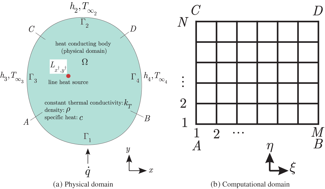
Figure 1: Irregular heat-conducting body (physical domain) subjected to a heat flux
The line heat source of time-varying strength
where
where
with the boundary and initial conditions
First the heat-conducting body is mapped from the irregular
where
where
The boundary and initial conditions can be transformed as
Using the finite difference method to discretize the derivatives in the resulting equations in the computational domain, we obtain (assuming
where
where
2.2 Steady-State Heat Conduction
With the same explanations for transforming the transient heat condition equation, we can obtain the transformed relations for the steady-state heat conduction equation. Then by substituting the finite difference expressions given in Eq. (16) into the obtained steady-state equation, and then solving for
where from Eq. (16),
3.1 Objective Function for Transient Heat Conduction
As in this study, two separate inverse heat transfer problems are considered (the transient and steady-state cases), the objective function expressions are defined separately for each case. For the transient heat transfer problem, the inverse analysis is concerned with the estimation of the time-varying line heat source strength
where
Sensitivity Analysis for Transient Heat Conduction
In this study, a gradient based minimization method (steepest descent method) is used to minimize the objective function value for both the transient and steady-state problems. Thus the gradient of the objective function with respect to the unknown variables is required. In the transient inverse problem, the gradient of the objective function
This is a function estimation problem and there is no prior information on the functional form of the unknown variable (here the line heat source strength
This implies that two variables at two different times
In Eq. (23),
thus
And Eq. (26) becomes
Now all the sensitivity coefficients
At any time
3.2 Objective Function for Steady-State Heat Conduction
For the steady-state case, the sensors are placed at the boundary
where
where the
Again, the sensitivity coefficients can be calculated using the chain rule as
The term
The term
Thus the sensitivity coefficients for the steady-state heat conduction case will be as
Sensitivity Analysis for Steady-State Heat Conduction
In this case, the sensitivity matrix Ja can be explicitly written as
3.3 Minimization: Steepest Descent Method
The steepest descent minimization method used in this study is expressed as
where
where the gradient direction
Minimization Algorithm
The inverse analysis steps proposed in this study to estimate the constant and time-varying line heat source strengths can be summarized as below:
1. The temperature measurements are taken at the sensor place
2. The direct problem is solved to obtain the temperature values at the sensor place and the time
3. The objective function (
4. The specified stopping criterion is examined for stopping or continuation of the minimization process.
5. The gradient direction
6.
The minimization process to estimate the unknown variables can be stopped when the objective function is minimized sufficiently and stable and satisfactory results are obtained. In this study the minimization process is terminated when the objective function value
where
The measured temperatures containing random errors
where
For each of the inverse transient and steady-state heat conduction problems, two test cases are presented. The data used in the test cases are so that they can reflect the accuracy, efficiency, and robustness of the proposed inverse analysis. At each test case, initially the direct heat conduction problem is solved with prescribed values of the line heat source strength to compute the temperature value at the sensor place. Then the computed temperatures are used as simulated measured ones to recover the prescribed values of the line heat source strength. For the function estimation problems (transient case), two different forms of timewise variation for the heat source are considered.
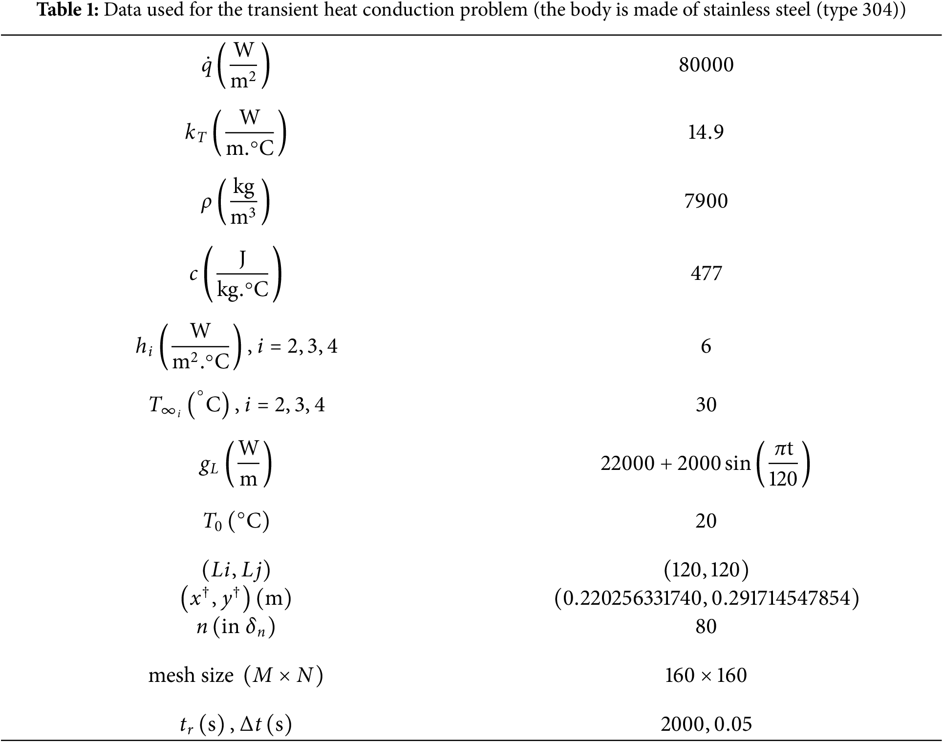
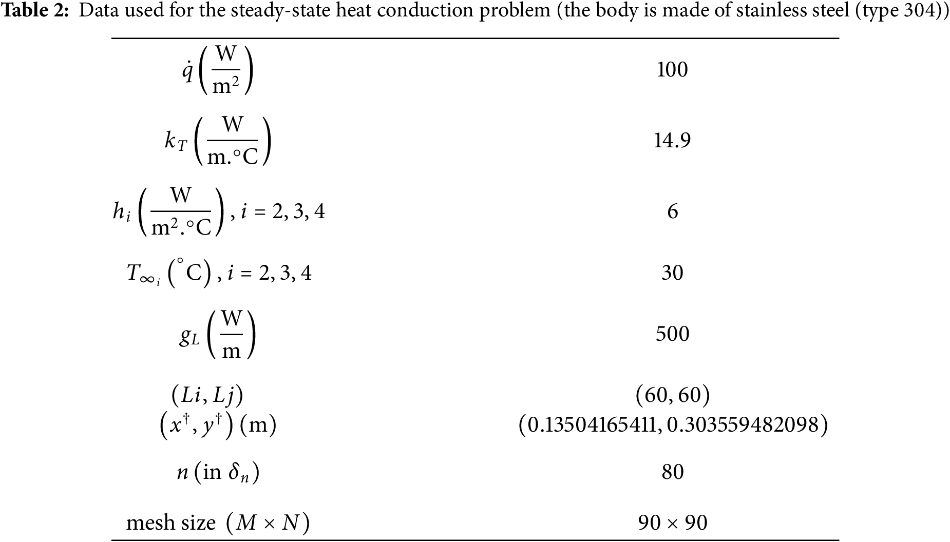
Before proceeding further, the steady-state and transient heat conduction equations are validated with the results from the commercial finite element software COMSOL. We assume that the heat conducting body is made of stainless steel (type 304) and the data used in the transient and steady-state test cases are listed in Tables 1 and 2, respectively. It should be added that all computations in this study are carried out using a Fortran compiler.
The temperature distribution in the irregular heat conducting body for the transient heat transfer problem using the explicit code used in this study and the software COMSOL is shown in Fig. 2. Moreover, the temperature distribution along a radial line passing over the heat source computed by our code and COMSOL (Fig. 3) are compared (Fig. 4). And the temperature distribution in the irregular heat conducting body for the steady-state heat transfer problem using the explicit code and COMSOL is shown in Fig. 5. It can be seen that the there is a good agreement between the results obtained from our code and the ones obtained from the software COMSOL confirming the accuracy of our code. Furthermore, the shape and the location of the function
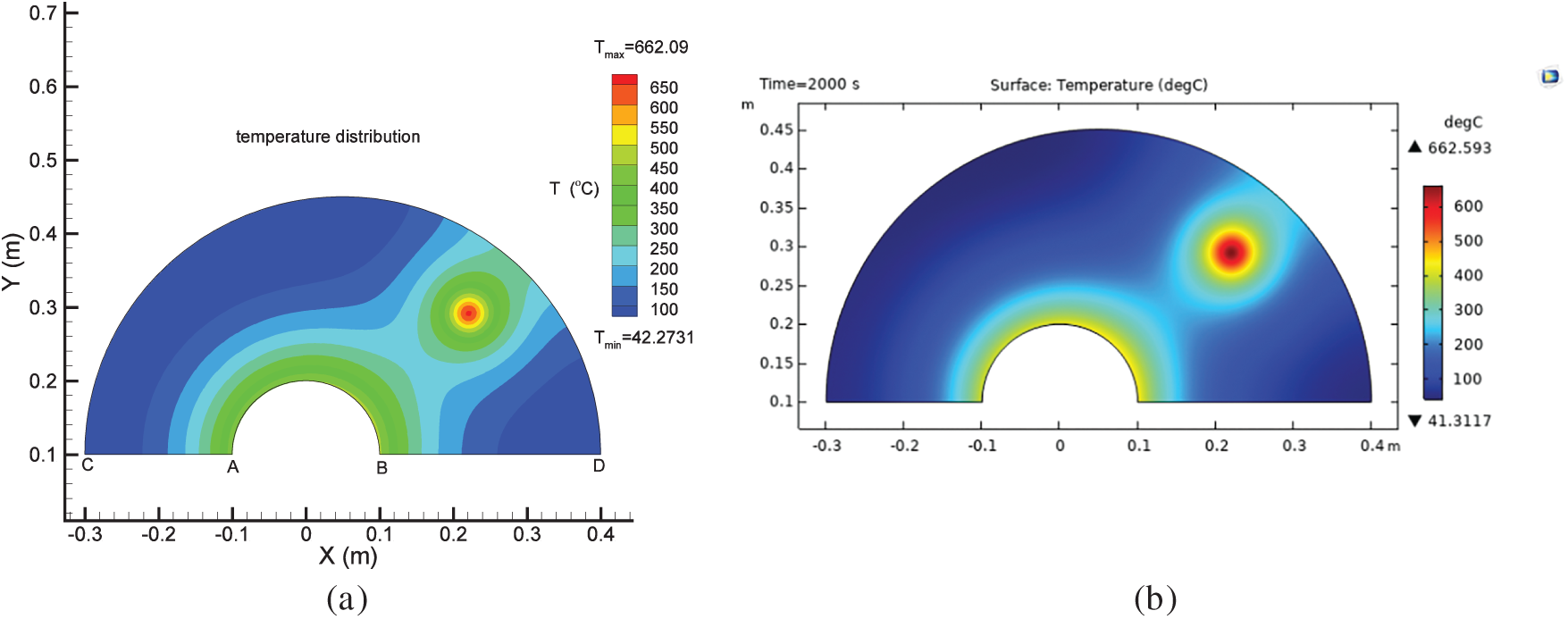
Figure 2: Validation of the transient heat conduction solver using the finite element software COMSOL. The result obtained by using our code (a) and the result obtained by using COMSOL (b)
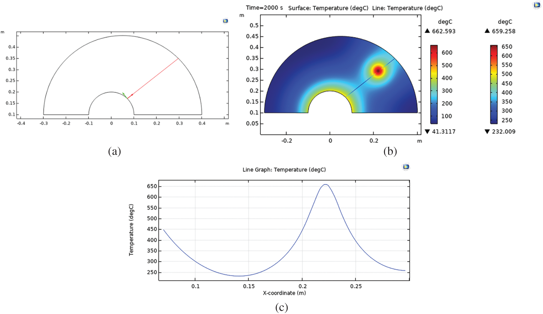
Figure 3: Temperature along a radial line passing over heat source obtained by software COMSOL. (a) the place of line (b,c) the temperature distribution

Figure 4: Comparison of temperature distribution along a radial line passing over heat source obtained by our code and software COMSOL

Figure 5: Validation of the steady-state heat conduction solver using the finite element software COMSOL. The result obtained by using our code (a) and the result obtained by using COMSOL (b)
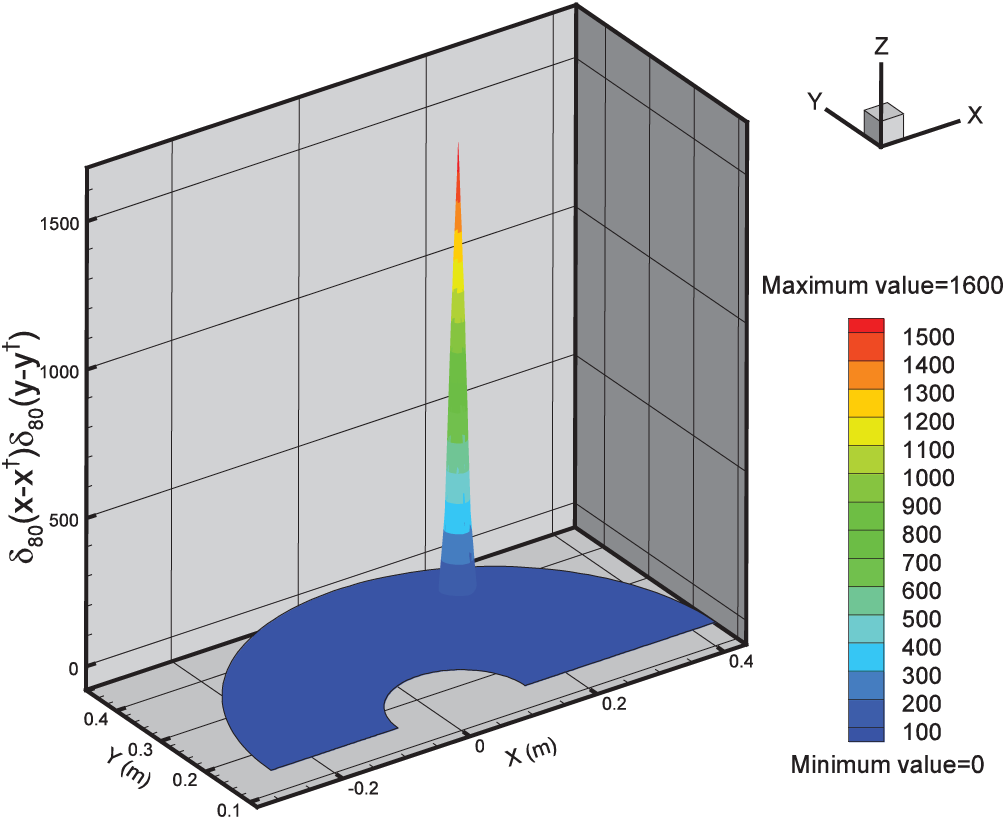
Figure 6: The shape and location of the function
4.1 Test Cases 1 & 2 (Transient)
As mentioned previously, initially the direct transient heat conduction problem is solved using prescribed values of the line heat source strength (
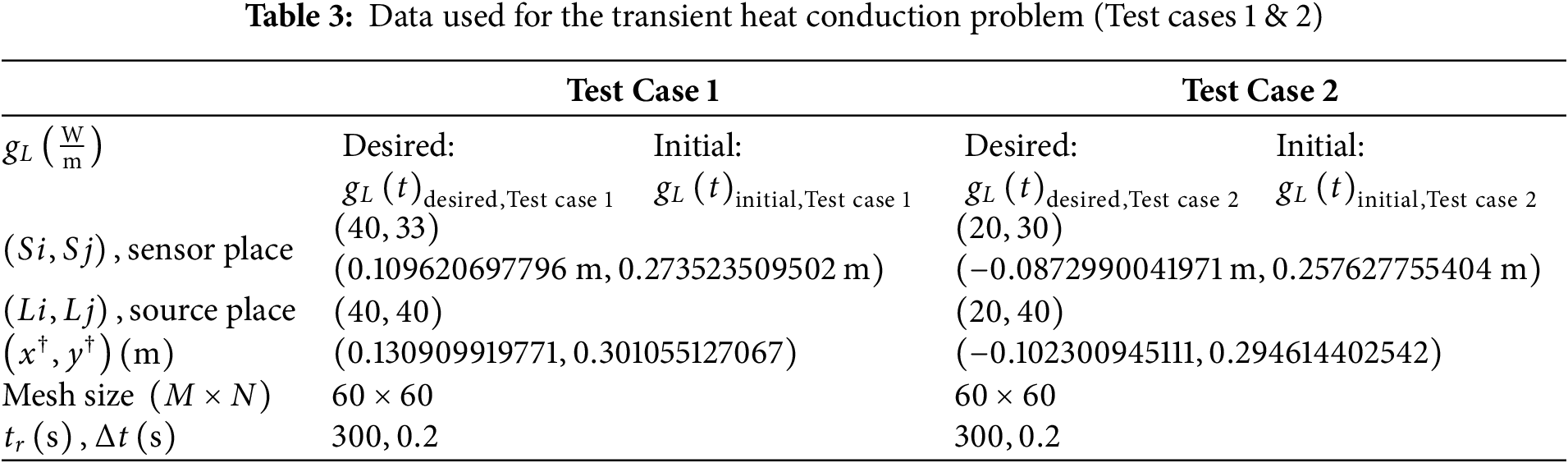
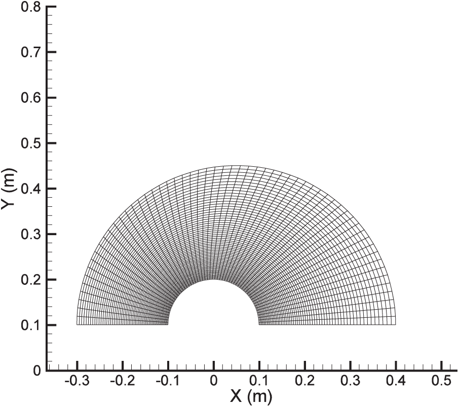
Figure 7: The physical domain and the grid size of
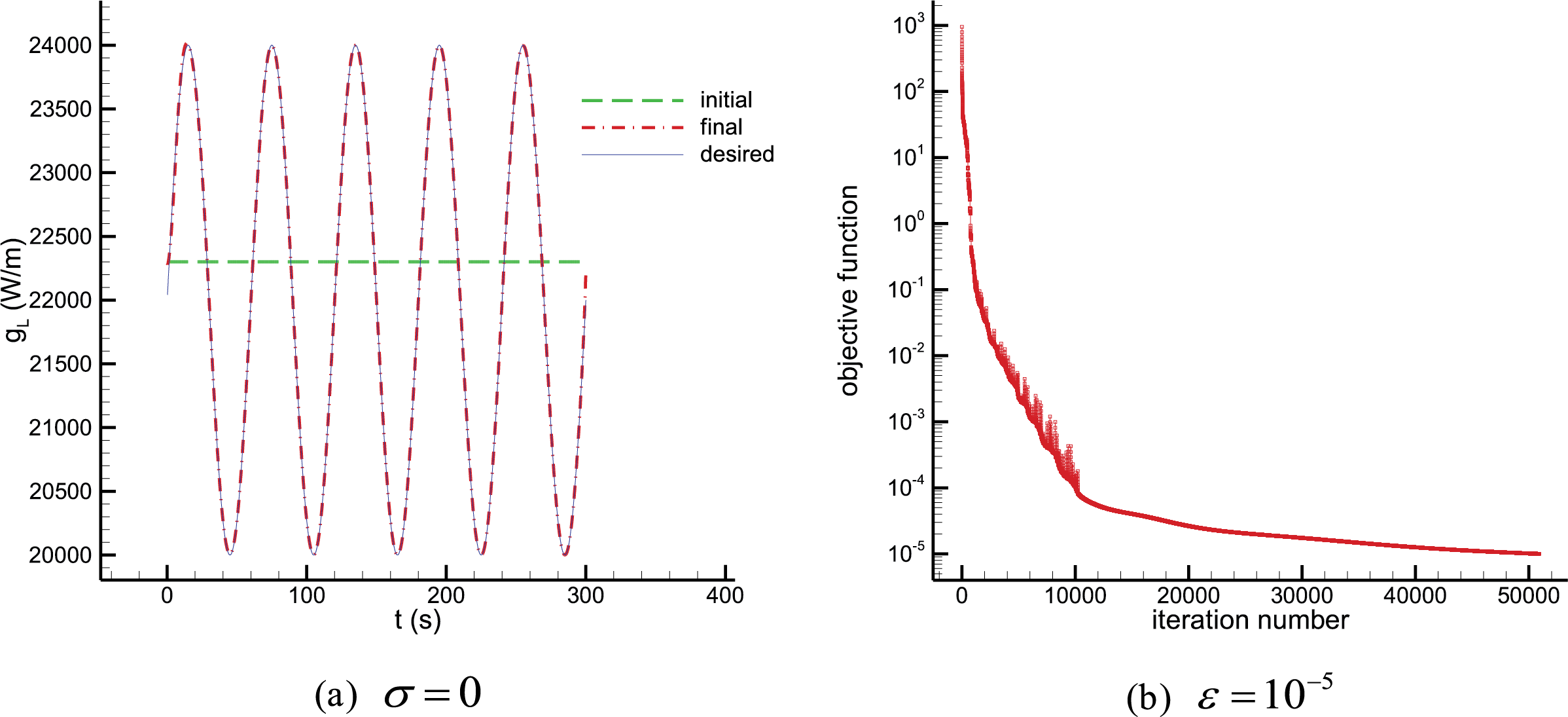
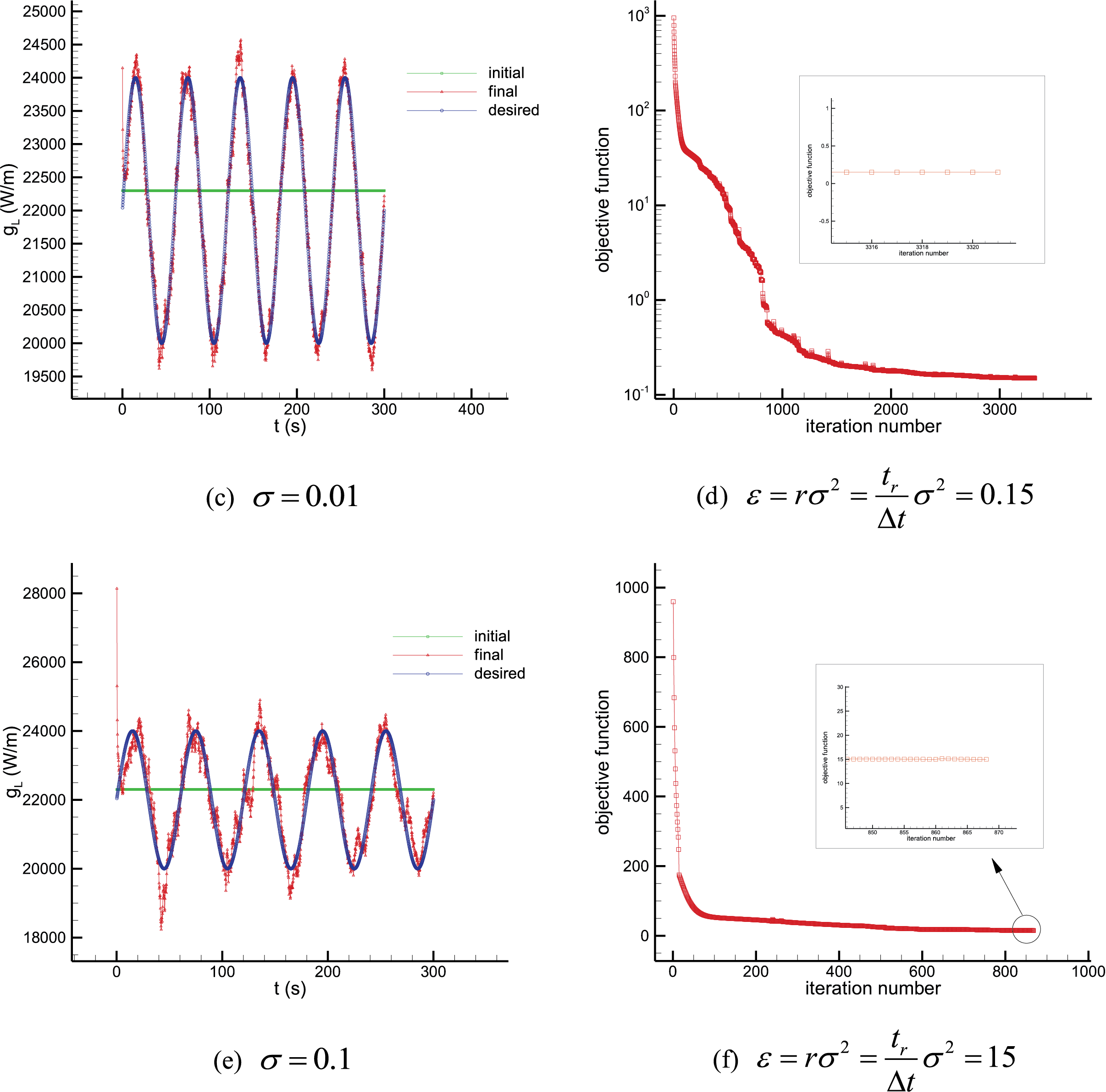
Figure 8: Test case 1 results. Estimation of the time-varying line heat source strength
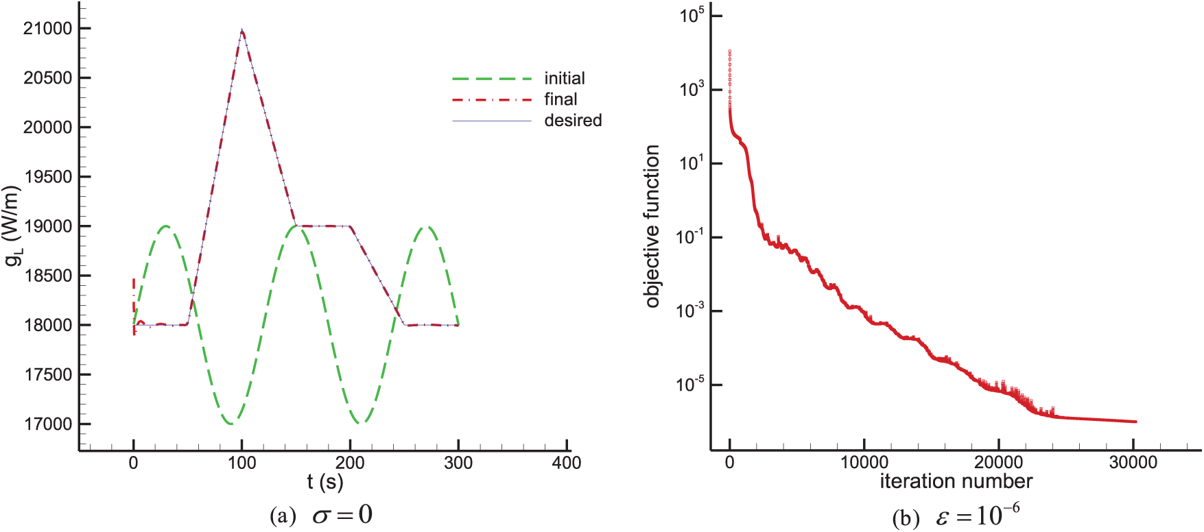
Figure 9: Test case 2 results. Estimation of the time-varying line heat source strength
From the results we can see that at the very early times
From Eq. (22),
which is a very small number. Substituting a very small value for
Now in order to further investigate the effect of the initial guess on the minimization process and the estimated variable, a different initial guess is considered which is far from the desired heat source value. Once again Test case 2 is considered with the following constant line heat source strength as an initial guess:
The result shown in Fig. 10 indicates the two points mentioned previously. Again, some deviations can be seen at very initial times as well as the final times. However, as it can be seen, the number of the deviated components of the estimated heat source is negligible compared to the total number of the components (which is
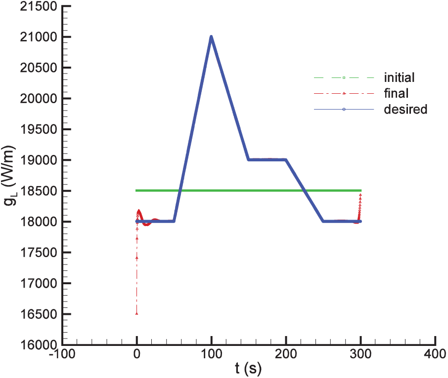
Figure 10: Test case 2 result. Estimation of the time-varying line heat source strength
4.2 Test Case 3 & 4 (Steady-State)
In Test cases 3 & 4, the objective is to recover the constant line heat source strength
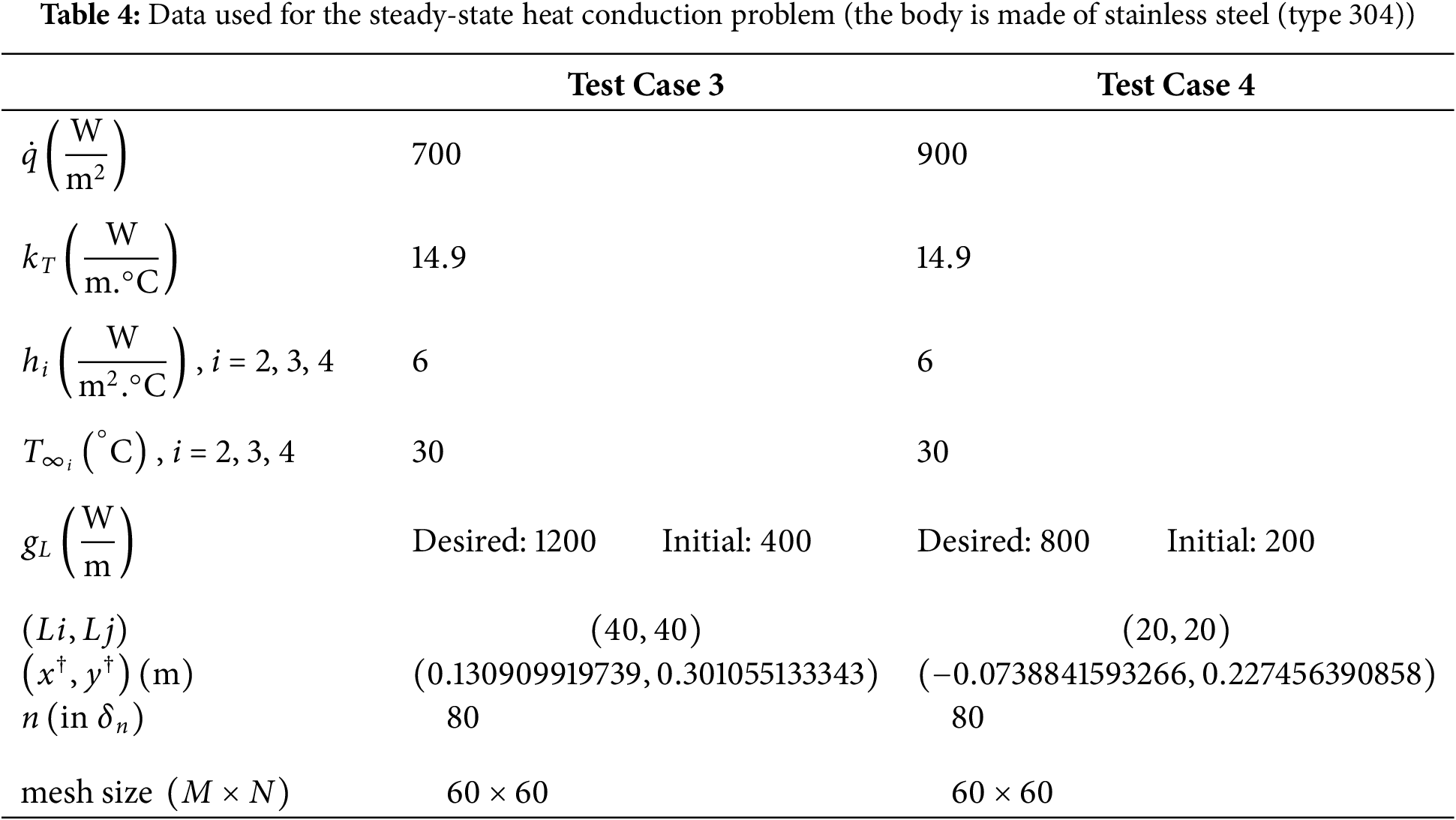
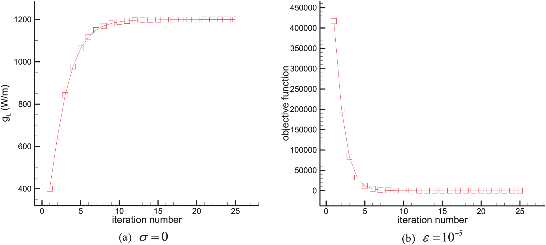
Figure 11: Test case 3 results. Estimation of the constant line heat source strength
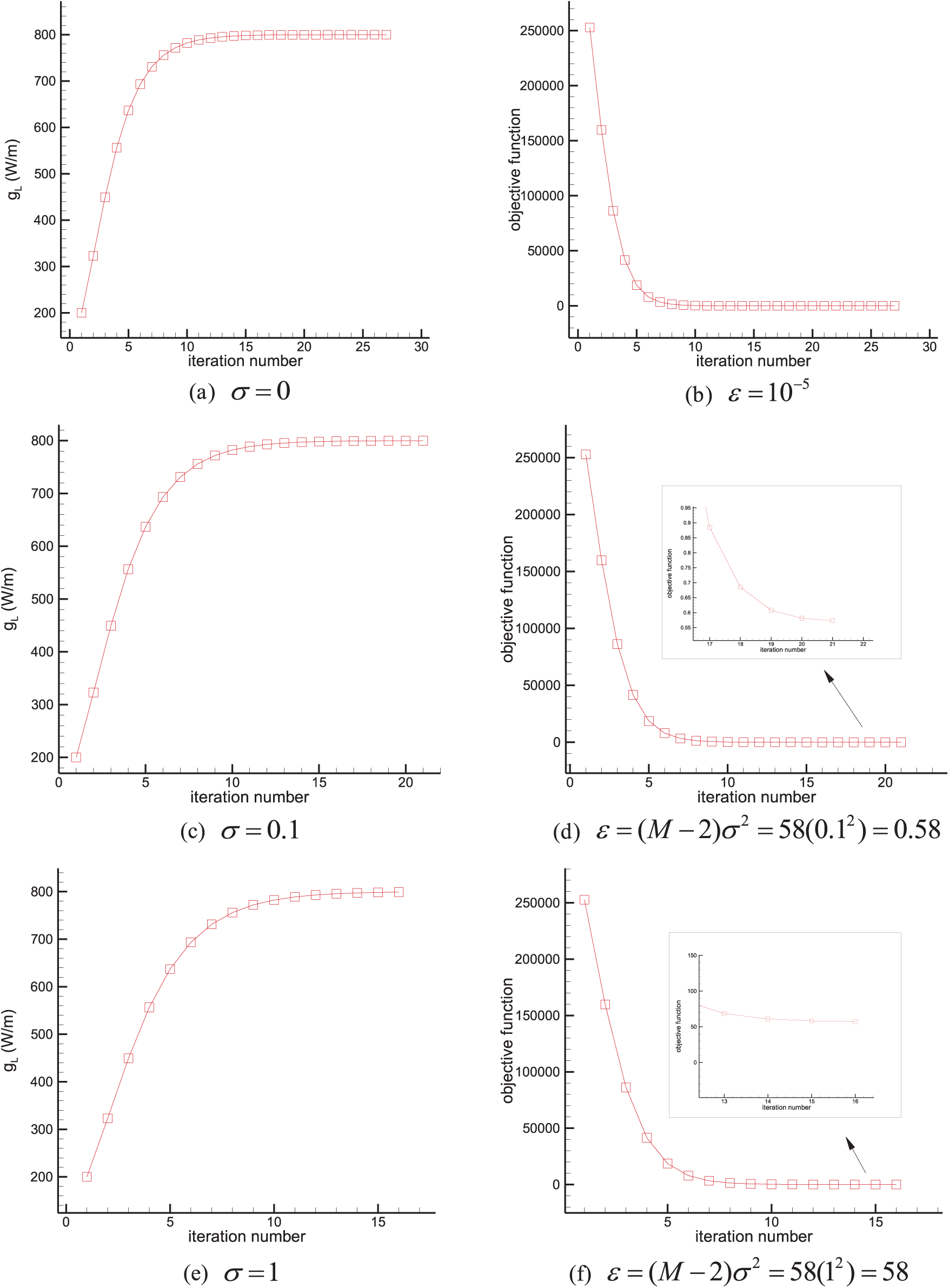
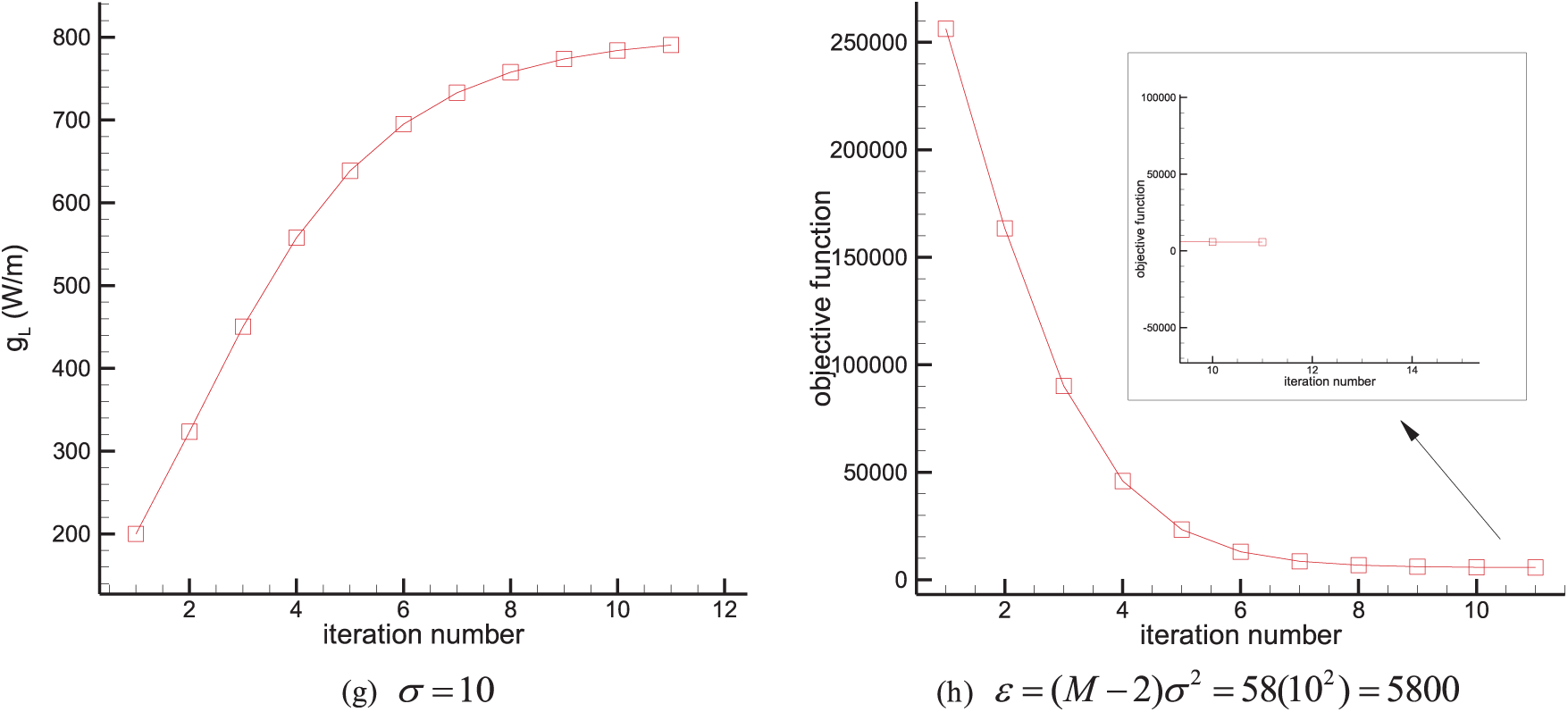
Figure 12: Test case 4 results. Estimation of the constant line heat source strength
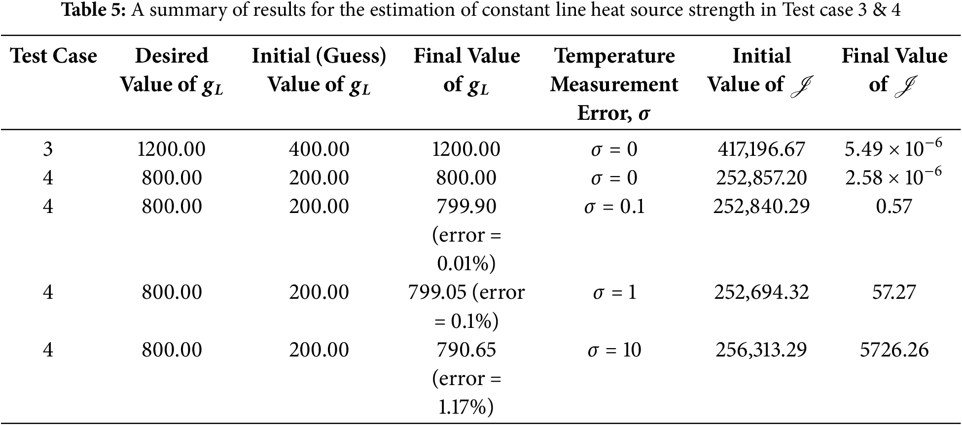
Inverse crime. To avoid committing an inverse crime, a different mesh is also used to recover the desired heat source in Test case 4 with the largest measurement error of
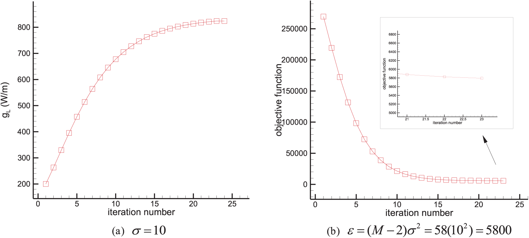
Figure 13: Test case 4 (different mesh size to avoid inverse crime) results. Estimation of the constant line heat source strength

and for the mesh of size
This study presented an adjoint free gradient based inverse analysis to estimate a line heat source strength in the transient (function estimation) and steady-state (parameter estimation) inverse heat conduction problems over general 2D heat conducting bodies with the Neumann and Robin boundary conditions. Since the domain shape was irregular, a body-fitted grid generation method was used to mesh the domain. Then the heat conduction equations and the associated boundary conditions were transformed from the irregular physical domain to the regular computational domain to be able to use the finite difference method to discretize the equations. In the inverse analysis, an objective function is defined based on the least squares norm. Then using the chain rule and direct differentiation, an efficient, accurate, and very easy to implement sensitivity analysis was developed which enabled us to compute all the sensitivity coefficients during the direct heat transfer solution using the explicit expressions without the need to solve the sensitivity and adjoint problems to obtain the gradient of the objective function with respect to the unknown variables thereby reducing the computational cost of the inverse analysis significantly. The steepest descent method was used to minimize the objective function. By considering some levels of the measurement error, a few test cases were presented to reveal the accuracy of the method. The results from the test cases showed that the proposed inverse analysis is very accurate, efficient, and robust. In the steady-state cases, the analysis was not affected significantly by the measurement error. However, there was a relatively large error in the estimated function in the transient test cases when the measurement error was large as well.
Acknowledgement: Not applicable.
Funding Statement: The author received no specific funding for this study.
Availability of Data and Materials: The data that supports the findings of this study are available from the author upon reasonable request.
Ethics Approval: Not applicable.
Conflicts of Interest: The author declares no conflicts of interest to report regarding the present study.
References
1. Özışık MN, Orlande HR. Inverse heat transfer: fundamentals and applications. Oxfordshire, UK: Taylor & Francis; 2000. [Google Scholar]
2. Alifanov OM. Inverse heat transfer problems. Berlin/Heidelberg, Germany: Springer Science & Business Media; 2012. [Google Scholar]
3. Mohebbi F. Function estimation in inverse heat transfer problems based on parameter estimation approach. Energies. 2020;13(17):4410. doi:10.3390/en13174410. [Google Scholar] [CrossRef]
4. Mohebbi F, Sellier M. Estimation of functional form of time-dependent heat transfer coefficient using an accurate and robust parameter estimation approach: an inverse analysis. Energies. 2021;14(16):5073. doi:10.3390/en14165073. [Google Scholar] [CrossRef]
5. Lu ZR, Pan T, Wang L. A sparse regularization approach to inverse heat source identification. Int J Heat Mass Transf. 2019;142(12):118430. doi:10.1016/j.ijheatmasstransfer.2019.07.080. [Google Scholar] [CrossRef]
6. Safari F, Duan Y. A novel meshless method in conjunction with a regularization technique for solving the transient heat source with additive noise. Int Commun Heat Mass Transf. 2024;158(25–26):107949. doi:10.1016/j.icheatmasstransfer.2024.107949. [Google Scholar] [CrossRef]
7. Wei X, Huang A, Sun L. Singular boundary method for 2D and 3D heat source reconstruction. Appl Math Lett. 2020;102:106103. doi:10.1016/j.aml.2019.106103. [Google Scholar] [CrossRef]
8. Lv C, Wang G, Chen H, Wan S. Estimation of the moving heat source intensity using the multiple model adaptive inverse method. Int J Therm Sci. 2019;138(3):576–85. doi:10.1016/j.ijthermalsci.2019.01.018. [Google Scholar] [CrossRef]
9. Karkhin VA. Thermal processes in welding. Berlin/Heidelberg, Germany: Springer; 2019. [Google Scholar]
10. Silva Neto AJ, Özişik MN. Two-dimensional inverse heat conduction problem of estimating the time-varying strength of a line heat source. J Appl Phys. 1992;71(11):5357–62. doi:10.1063/1.350554. [Google Scholar] [CrossRef]
11. Park HM, Chung OY, Lee JH. On the solution of inverse heat transfer problem using the Karhunen-Loève Galerkin method. Int J Heat Mass Transf. 1999;42(1):127–42. doi:10.1016/s0017-9310(98)00136-7. [Google Scholar] [CrossRef]
12. Jarny Y. Determination of heat sources and heat transfer coefficient for two-dimensional heat flow—numerical and experimental study. Int J Heat Mass Transf. 2001;44(7):1309–22. doi:10.1016/s0017-9310(00)00186-1. [Google Scholar] [CrossRef]
13. Liu FB. A modified genetic algorithm for solving the inverse heat transfer problem of estimating plan heat source. Int J Heat Mass Transf. 2008;51(15–16):3745–52. doi:10.1016/j.ijheatmasstransfer.2008.01.002. [Google Scholar] [CrossRef]
14. Gu Y, Lei J, Fan CM, He XQ. The generalized finite difference method for an inverse time-dependent source problem associated with three-dimensional heat equation. Eng Anal Bound Elem. 2018;91(1):73–81. doi:10.1016/j.enganabound.2018.03.013. [Google Scholar] [CrossRef]
15. Yan L, Fu CL, Yang FL. The method of fundamental solutions for the inverse heat source problem. Eng Anal Bound Elem. 2008;32(3):216–22. doi:10.1016/j.enganabound.2007.08.002. [Google Scholar] [CrossRef]
16. Hazanee A, Lesnic D, Ismailov MI, Kerimov NB. An inverse time-dependent source problem for the heat equation with a non-classical boundary condition. Appl Math Model. 2015;39(20):6258–72. doi:10.1016/j.apm.2015.01.058. [Google Scholar] [CrossRef]
17. Shah S, Parwani AK. Estimation of time-varying heat source for one-dimensional heat conduction by conjugate gradient method. In: Innovations in infrastructure. Singapore: Springer; 2018. p. 329–39. doi:10.1007/978-981-13-1966-2_29. [Google Scholar] [CrossRef]
18. Lee KH. Application of repulsive particle swarm optimization for inverse heat conduction problem—parameter estimations of unknown plane heat source. Int J Heat Mass Transf. 2019;137:268–79. doi:10.1016/j.ijheatmasstransfer.2019.03.092. [Google Scholar] [CrossRef]
19. Min T, Zang S, Chen S. Source strength identification problem for the three-dimensional inverse heat conduction equations. Inverse Probl Sci Eng. 2020;28(6):827–38. doi:10.1080/17415977.2019.1665663. [Google Scholar] [CrossRef]
20. Necati OM. Heat conduction. Hoboken, NJ, USA: John Wiley & Sons; 1993. [Google Scholar]
21. Ozisik MN. Finite difference methods in heat transfer. Boca Raton, FL, USA: CRC Press; 1994. [Google Scholar]
22. Mohebbi F, Sellier M. Viscosity and effusion rate identification from free surface data. Int J Thermofluids. 2022;15:100184. doi:10.1016/j.ijft.2022.100184. [Google Scholar] [CrossRef]
Cite This Article
 Copyright © 2025 The Author(s). Published by Tech Science Press.
This work is licensed under a Creative Commons Attribution 4.0 International License , which permits unrestricted use, distribution, and reproduction in any medium, provided the original work is properly cited.
 Downloads
 Citation Tools