Temperature Prediction of the Clamp-Conductor Coupling Zone in Transmission Lines

1  Introduction

As global power demand continues to rise, some power grids have driven transient line ampacity to their design limits in order to maximize capacity [1]. However, current ampacity standards—based on limiting bulk conductor temperature to below 70°C (or 120°C under special conditions) [2]—do not account for operational thermal non-uniformity. Localized overheating at clamp-conductor interfaces is frequently observed and is attributed to anomalies in contact resistance [3]. These thermal hotspots initiate feedback loops of accelerated metal oxidation and interfacial micro-deformation, increasing contact resistance and precipitating sustained arcing damage—key failure mechanisms in power lines [4]. Empirical studies report thermal gradients of 15°C–30°C between dynamically overloaded clamps and adjacent conductor segments [5]. Such temperature differentials lead to cascading effects: up to 40% reduction in clamping force, a 3–5-fold increase in creep-rupture probability, and substantial Joule heating losses [6]. In transmission assets older than 25 years, the combined effects of interfacial oxide accumulation and stress relaxation render clamp zones the primary constraints on ampacity and service life [7]. Therefore, comprehensive characterization of interfaces is essential for ensuring grid reliability and developing robust dynamic capacity enhancement strategies [8].

Over the past decade, research on clamp temperature behavior has focused on two principal areas: spatial temperature distribution and transient temperature rise. The first area investigates the spatial temperature distribution and steady-state thermal behavior of various clamp designs. Lin et al. employed both experiments and simulations to map cross-sectional temperature profiles of clamps under diverse environmental conditions, highlighting pronounced non-uniformity in temperature fields [9]. Angadi et al. examined temperature rise in electrical connectors, incorporating contact resistance variations as a function of contact pressure [10]. Zhang developed a 1:1 multiphysics simulation of the 2756/SJ1503 insulating jumper clamp—coupling electrical, thermal, and mechanical phenomena—and validated the model experimentally by varying contact pressure, ambient temperature, light intensity, wind speed, and load current [11]. He et al. proposed a coupled mechanical–thermal–electrical framework for parallel-groove clamps, analyzing temperature rise under both steady and impulse high-current conditions [12]. Jian performed temperature-rise and thermal-cycling experiments on strain clamps and tension joints, correlating resistance fluctuations with cycle count to elucidate degradation mechanisms [13]. Mo-hung, W et al. investigated corrosion-induced temperature rise in load-bearing clamp hardware exposed to acidic and alkaline salt-ion fog, identifying key environmental factors that exacerbate heating [14]. Liao et al. studied clamp surface temperature increase under varying corrosive solution pH and concentration across different current loads, providing insights into environmental and electrical coupling effects.

Previous studies have largely focused on individual clamps, overlooking heat transfer between clamps and conductors [15]. The second research area examines the temperature-rise behavior of overhead conductors equipped with clamps. Tan et al. analyzed the circular current-density distribution in the clamp contact zone, finding that the resulting ring-shaped heat source induces thermal-stress concentrations at the periphery, which can initiate cracking and fracture [16]. Bühlmann et al. characterized temperature profiles of conductors around tension clamps and adjacent spans, and further simulated AAAC axial temperature distribution in the vicinity of wedge-shaped clamps [17,18]. Dong examined the effect of bolt torque on clamp resistance and thermal distribution, reporting that elevated clamp temperatures raise conductor temperatures and may limit transmission capability [19]. Using ANSYS, Beloufa assessed the impact of cable cross-sectional area on connector temperature rise, showing that an optimal area minimizes contact resistance and thermal elevation, thereby prolonging connector life [20]. Considering the higher operating temperatures of HTLS conductors, Soppe et al. developed a computational framework to reassess mechanical accessory standards, enabling simulations of steady-state temperature profiles under realistic loading conditions [21]. Jin et al. identified thermal-imaging signatures of inadequate conductor-clamp contact that precede melting failures in overhead systems [22]. Yang et al. proposed an intelligent diagnostic system for detecting overheating faults, specifically targeting thermal anomalies between tension clamps and conductors [23]. Wang et al. analyzed the physical process of ice melting on conductor structures from a heat transfer perspective, established a simplified mathematical model for conductor ice melting under gravity free conditions, and derived analytical expressions for the temperature distribution across various parts of the conductor when it reaches a steady state of ice melting [24]. Zhou et al., based on the internal structural characteristics of overhead conductors, analyzed the radial temperature of conductors under natural convection, laminar flow, and turbulent flow conditions, and obtained a more accurate calculation method for the core temperature of conductors [25]. While previous studies have examined the temperature-rise characteristics of clamps or conductors equipped with clamps, a precise analysis of temperature behavior in the clamp-conductor coupling region and its surroundings is still lacking. Although thermal performance near clamps is less critical for short-term sag and rated capacity calculations, it is crucial for predicting conductor lifespan [26]. Therefore, this work adopts a conventional thermal modeling approach for overhead lines to develop an axial micro-element thermal-circuit model specific to the clamp-conductor coupling zone. The Whale Optimization Algorithm (WOA) is employed to identify unknown parameters within the thermal-circuit model, thereby improving parameter estimation accuracy. Simulated temperature-rise profiles are then compared with experimental measurements to validate model accuracy. By characterizing temperature distribution in the clamp-conductor coupling region, this study enables early detection of potential overheating issues. Furthermore, when assessing capacity upgrades for aged conductors, the model accurately predicts temperatures in critical zones, providing essential data to evaluate and maximize dynamic capacity enhancement potential.

Establishing a thermal model to predict temperature distribution in the clamp-conductor interface involves three principal stages, as depicted in Fig. 1.

•   The governing equations of the thermal model are derived from a detailed heat-transfer analysis of both the clamp and the conductor.

•   Thermal parameters—such as heat capacity and axial thermal resistance of the clamp and conductor—are determined experimentally under natural convection conditions and constant illumination to ensure high accuracy.

•   The WOA algorithm is then applied to identify remaining unknown parameters from experimental data, and the validated model is employed to compute temperature distribution in the clamp-conductor interface, thereby assessing the accuracy of the parameter identification.

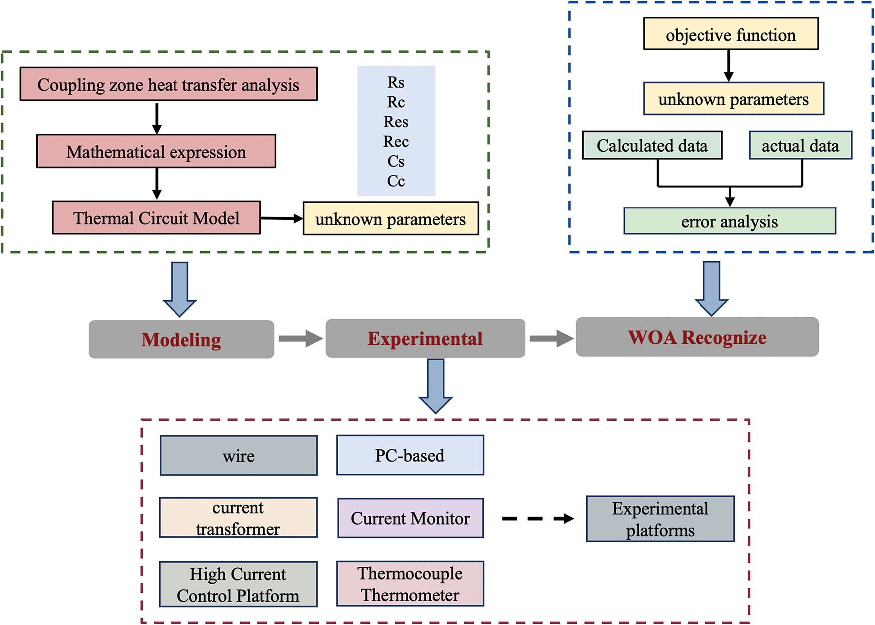
Figure 1: Research logic flow chart

This study completes the first two essential steps, which are prerequisites for the final validation phase. A thermal model for the clamp-conductor interface has been developed to predict temperature distribution at their contact region. In laboratory experiments conducted under natural convection and constant illumination, the WOA parameter-identification technique was applied to calibrate the model’s thermal parameters. Experimental results under these controlled conditions validate both the WOA-based parameter calibration and the accuracy of the thermal model. This work establishes a robust foundation for accurately predicting temperature distributions in clamp-conductor interfaces under realistic meteorological conditions and for supporting dynamic capacity enhancement of overhead conductors.

2  Equivalent Thermal Network for Clamp-Conductor Coupling

2.1 Conventional Thermal Mode

Overhead conductors’ temperature is governed by wind speed and direction, ambient air temperature, solar irradiance, and the magnitude of electrical current. According to IEEE Standard 738, conductor thermal behavior is modeled by a first-order differential equation [27] that balances absorbed and dissipated heat:

CcdTcdt=𝒬Jc+𝒬sc−𝒬rc−𝒬cc.(1)

Heat removal from the clamp occurs through conduction, convection, and radiation [28]. Accordingly, the clamp’s thermal response is modeled by a first-order differential equation:

CsdTsdt=𝒬Js+𝒬ss−𝒬rs−𝒬cs.(2)

In this context, Tc and Ts denote the conductor and ambient temperature (°C) respectively. Cc and Cs represent the thermal capacitances of the conductor and clamp, respectively (J/m·°C). QJc and QJs correspond to Joule heating in the conductor and clamp (W/m), while Qsc and Qss denote solar heat gains for the conductor and clamp (W/m). Convective (Qcc, Qcs) and radiative (Qrc, Qrs) losses for the conductor and clamp are represented in W/m.

2.2 Development of Equivalent Thermal Network

To model axial temperature distribution in the clamp-conductor interface, an equivalent thermal-network approach is adopted to represent thermal equilibrium between the clamp and the conductor. Compared to conventional methods such as finite-element, finite-volume, and finite-difference analyses, the equivalent thermal-network approach offers reduced computational complexity and simpler implementation [29].

Fig. 2 outlines the two step process for constructing an equivalent thermal-network model for the clamp–conductor interface:

Figure 2: Equivalent thermal network

First, the clamp and conductor in the interface region are divided into axial micro-elements of uniform length based on thermal equilibrium and anticipated temperature gradients.

Because the conductor diameter is negligible relative to its length, radial temperature gradients within the conductor are neglected. Thus, the micro-elements length determines spatial resolution and should be selected according to engineering requirements. Fig. 2 also presents a schematic of axial micro-element heat transfer in the clamp-conductor interface. Here, i indexes each micro-element. Specifically, Qcc, Qrc, QJc, Qsc, and Qds denote heat flows in conductor micro-elements, whereas QJs, Qrs, Qss, Qcs correspond to clamp micro-elements.

Based on the principle of thermal equilibrium, each micro-element shown in Fig. 3 exchanges heat both with its environment and with adjacent micro-elements [30]. Consequently, the thermal-balance equation for micro-element i can be expressed as follows:

ρCidTc,idt=𝒬Js,i+𝒬ss,i+𝒬dc,i+1−𝒬rs,i−𝒬cs,i−𝒬ds,i.(3)

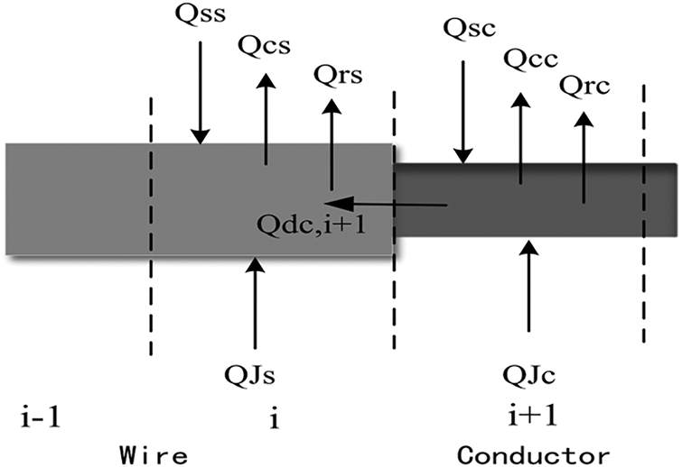
Figure 3: Axial heat transfer model

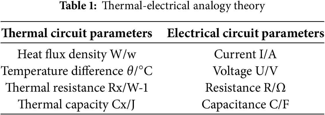
In this context, ρ denotes density; Tc,i is the temperature at the center of micro-element i (°C), and Ci represents its equivalent thermal capacitance (J/°C). Qdc,i+1 denotes conductive heat flow from element i + 1 into element i, while Qds,i denotes conductive heat flow from element i into i − 1. QJs,i and Qss,i correspond to Joule heating and solar heat gain of element i, respectively; Qcs,i and Qrs,i represent its convective and radiative losses. After constructing the equivalent thermal network, the thermal-balance equations are solved using the thermoelectric-analogy framework, which maps thermal quantities to electrical analogues, as detailed in Table 1.

Building on this framework, the heat flows Qdc,i+1, Qds,i, Qcs,i, and Qcc,i+1 in Eq. (3) are represented using Ohm’s law, as expressed in Eq. (4).

{𝒬dc,i+1=Ts,i+1 − Ts,iRc𝒬ds,i=Ts,i − Ts,i−1Rs𝒬cs,i=Ts,i − Te,iRes𝒬cc,i+1=Tc,i+1 − Te,i+1Rec.(4)

In this context, Rc and Rs denote the equivalent conductive thermal resistances between adjacent micro-elements (°C/W), while Res and Rec represent the equivalent convective resistances between micro-elements and the ambient environment (°C/W). Additionally, Te,i and Te,i+1 denote the ambient temperatures at micro-elements i and i + 1, respectively (°C).

Consequently, the thermal-balance equation for micro-element i can be reformulated as follows [31]: The analysis utilizes differential elements comprising the clamp element at position i, the conductor segment at position i–1, and the conductor segment at position i + 1:

ρCsdTs,idt=𝒬Js,i+𝒬ss,i+Tc,i+1−Ts,iRc−𝒬rs,i−Ts,i−Te,iRes−Ts,i−Ts,i−1Rs.(5)

Similarly, the thermal-balance equation for micro-element i + 1 can be expressed as: the differential elements used consist of the clamp element at position i, and the conductor elements at positions i + 1 and i + 2:

ρCcdTc,i+1dt=𝒬Jc,i+1+𝒬sc,i+1−Tc,i+1−Ts,iRc−𝒬rc,i+1−Tc,i+1−Te,i+1Rec−Tc,i+1−Tc,i+2Rc.(6)

By assembling the thermal-balance equations for each micro-element, an equivalent thermal-network model of the clamp-conductor interface region is constructed, as shown in Fig. 4.

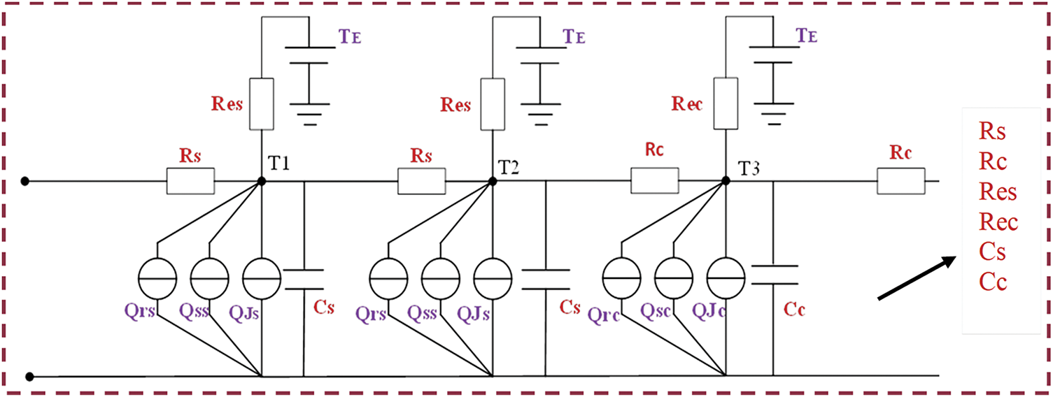
Figure 4: Equivalent thermal network

3  Determination of Thermal Parameters

Before implementing the equivalent thermal network model for the clamp-conductor interface, it is necessary to identify the relevant thermal parameters: QJ, Qs, Qr, Res, Rec, Rs, Rc, Cs, and Cc. Parameters QJ, Rs, Rc, Cs, and Cc are intrinsic to the materials and geometry and thus are independent of weather conditions.

In contrast, Qs, Qr, Res, and Rec depend on environmental variables such as solar irradiance, ambient temperature, wind speed, and wind direction. Within the thermal-network framework, micro-element heat flows QJs,i, QJc,i+1, Qss,i, and Qrs,i are calculated using Eq. (7). Similarly, Qsc,i+1 and Qrc,i+1 are obtained by the same procedure:

{𝒬Jc=I2R(T)=I2ζIτR20[1+α(T−20)]QJs=I2ρLS𝒬s=δ𝒬sesin(θ)A′𝒬r=σFijεiA′(Tw4−Te4).(7)

Here, 𝒬Jc is the Joule heat of the conductor, 𝒬Js is the Joule heat of the clamp, Qs is the solar heat gain, and Qr is the radiation loss. In the equation, I is the current flowing through, in amperes (A); R(T) is the AC resistance of the conductor at temperature T. ζ and τ are constants related to the standard cross-section of the conductor, and α is the temperature coefficient of the clamp resistance, in °C−1. According to the parameter table of LGJ-type steel-cored aluminum stranded wire, the DC resistance of the overhead conductor at 20°C is 0.1181 Ω/km, ζ = 0.8957, α = 0.01912, and R20 is the DC resistance of the conductor at 20°C, with a value of 0.1152 Ω/km. From the above formula, the heating power 𝒬Jc of the conductor can be calculated.

ρ is the AC resistivity of the clamp element, with a value of 2.82 × 10−8 Ω·m; L is the calculated length of the clamp, in meters; S is the radial cross-sectional area of the element, in square meters. Through measurement, the effective length L of the current passing through the clamp is 0.32 m, and the cross-sectional area S is 1.451 × 10−3 m2. δ is the solar absorptance, ranging from 0.23 to 0.91; 𝒬se and A′ are the solar heat power (W/m2) and the surface area of the object (m2), respectively. σ is the Stefan-Boltzmann constant, Fij is the shape factor; εi is the emissivity; Tw is the temperature of the heat source; Te is the ambient temperature, typically set at 25°C.

Although non-weather-dependent parameters Rs, Rc, Cs, and Cc can in theory be derived from their physical definitions, practical determination in engineering practice is challenging. This difficulty stems from the conductor’s construction—typically cylindrical aluminum and steel strands with inter-strand gaps and contact thermal resistances—which complicate axial heat transfer and thus precise computation of thermal capacitance and resistance. In contrast, the environmental thermal resistance Re depends dynamically on the temperature gradient between the conductor and the ambient surroundings and varies with meteorological conditions. Since exponential functions can capture both linear and nonlinear parameter variations, Re as a function of time step k is expressed as:

Re(k)=a(T(k)−Te(k))b.(8)

The coefficient a is a proportionality factor determined by conductor material properties, geometric dimensions, and air density, whereas b is an exponential factor typically set to −0.25. To accurately determine Res,a, Rec,a, Rs, Rc, Cs, and Cc, a WOA-based parameter-identification method is proposed to estimate these unknowns with high precision.

4  Parameter Identification of WOA

Due to the complexity of the proposed thermal circuit model—which involves numerous parameters and constitutes a nonlinear optimization problem—this study adopts the WOA [32] to optimize the objective function effectively. Fig. 5 illustrates the detailed flowchart of the WOA-based parameter identification process.

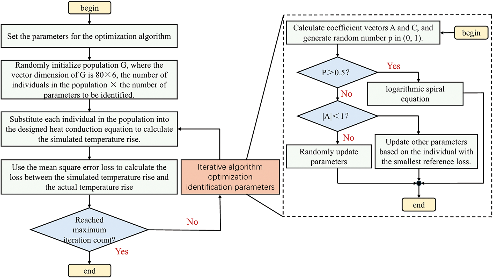
Figure 5: Parameter identification logical flowchart

First, the candidate solution set G is defined as:

G={⋃i=1nPi|Pi∈R6,n∈N,∀1≤i≤n}.(9)

Here, N denotes the number of candidate solutions, which is set to 80 in this study. The search space R6 comprises the six parameters to be identified: Res,a, Rec,a, Rs, Rc, Cs, and Cc. Each member of the solution set represents a potential parameter vector subject to iterative optimization.

In the first iteration, all individuals in population G are randomly initialized, i.e., G[i, 0:6] (0 ≤ I < 80) is randomly initialized, and the vector dimension of G is 80 × 6. Subsequently, G is entered into the temperature rise model to obtain the simulated temperature rise data for each individual. The specific process is as follows:

The temperature of the clamp and conductor at time K + 1 is equal to the temperature at time K plus the temperature rise. The initial value of the simulated temperature (at K = 0) is assigned as the initial value of the experimental temperature. Subsequently, the 6 initialized identification parameters and the initial simulated temperature are respectively substituted into Eqs. (5) and (6) to obtain the temperature rise. Through calculation step by step at each time interval, the final simulated temperature rise curves of the clamp and conductor are obtained.

The calculation formulas for the simulated clamp temperature and simulated conductor temperature at each time step are as follows:

Ts(k+1)=Ts(k)+dTs,idt,(10)

Tc(k+1)=Tc(k)+dTc,i+1dt.(11)

Once the simulated temperature rise curve is obtained, the mean square error between it and the specific experimental data is calculated, with the formula as follows:

Loss=∑k=060⁡[0.6∗||T~s(k+1)−Ts(k+1)||+0.4∗||T~c(k+1)−Tc(k+1||)].(12)

In this equation, T~s(k+1) and T~c(k+1) denote the experimentally measured temperatures of the splice clamp and conductor, respectively, at time step k + 1. Ts(k+1) and Tc(k+1) denote the experimentally simulated temperature of the splice clamp and conductor, respectively, at time step k + 1. To minimize the impact of environmental variability, all data were obtained under controlled indoor conditions—no solar radiation, no forced airflow, and constant ambient temperature—ensuring natural-convection heat transfer. Using the WOA algorithm, the loss function is iteratively optimized until convergence, yielding the identified parameters and finalizing the thermal-circuit model for the axial coupling region between the splice clamp and the conductor.

The loss obtained from Formula (12) is taken as the population fitness of each whale. Fitness values are then ranked, and the solution with the minimum loss is selected as the leader (local optimum) for the current iteration. Subsequently, each solution’s position is updated based on the WOA (Formula (13)) update rules, yielding the updated solution swarm after one iteration. Through successive iterations, the global optimum is eventually identified.

WiN={|W0N−1−WiN−1|⋅ebl⋅cos⁡(2πl)+W0N−1,P≥0.5W0N−1−A⋅|C⋅W0N−1−WrN−1|,P<0.5,(13)

here, W0N denotes the best solution (local optimum) from the previous iteration, while WiN and WrN are two candidate solutions, with the selection of WrN determined by the coefficient A. When p ≥ 0.5, each solution is updated along a logarithmic spiral path, where b controls the spiral tightness and r is a random variable uniformly distributed in [−1, 1]. If p < 0.5, all candidates move incrementally toward the current best (local optimum), using it as the reference point. The coefficient A governs the selection of the reference candidate WrN in Eq. (13): when A ≥ 1, r within WrN may be any member of the population; when A < 1, WrN = WiN, r is drawn from non-optimal candidates.

Through the optimization of the above-mentioned whale algorithm, a new set of identification parameters is obtained. These identification parameters are re-substituted into the temperature rise model to generate a new simulated temperature rise curve. The loss between this simulated temperature rise curve and the experimental data is calculated to guide the next iteration of the whale algorithm. After several iterations, the 6 identification parameters gradually converge, and the simulated temperature rise curve gradually fits the experimental data.

5  Equations and Mathematical Expressions

5.1 Experimental Platform

This study developed an experimental platform to validate the proposed thermal model and identify its thermal parameters. Fig. 6 shows the schematic and field-assembly diagrams of the platform.

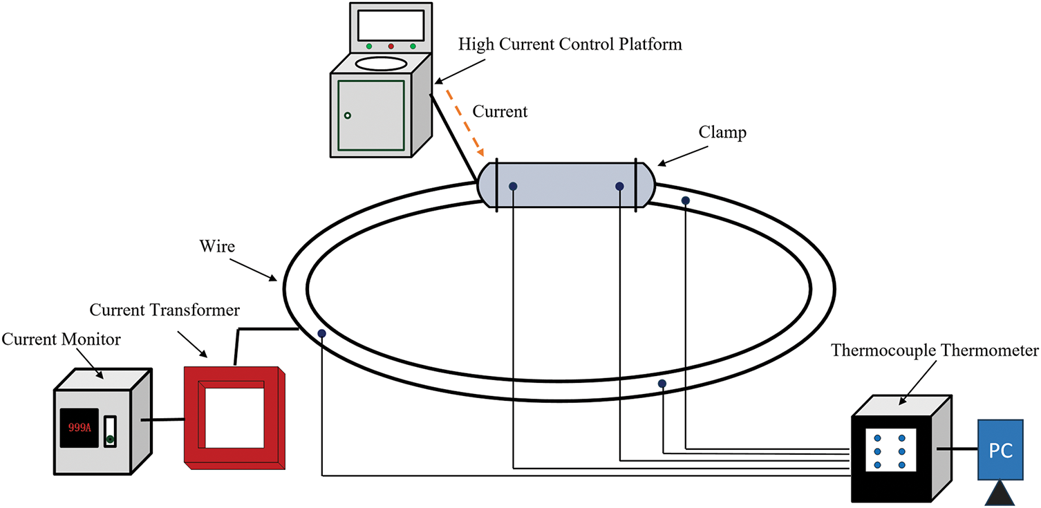
Figure 6: Experimental platform structure diagram

The setup was housed in a 5 m × 4 m × 3 m laboratory chamber where air velocity was maintained below 0.1 m/s to ensure natural-convection conditions. Ambient temperature and relative humidity were maintained at 25°C ± 0.5°C and 60% ± 1%, respectively. Radiative heat transfer was considered negligible under these indoor conditions due to minimal wind and no solar irradiance [33].

As shown in Fig. 7, the platform comprises a single-phase induction voltage regulator, a single-phase transformer, a 12-channel temperature data logger, a zero-sequence current transformer (class 10P), and the test conductors. Among them, the model of the 12-channel temperature tester is VX5112R/C2/U, and the power supply is 220VAC/50HZ. The model number of the temperature sensor is Temperature Range −73°C~705°C, Core diameter 2 ∗ 0.5 mm, Outer diameter 1.4 ∗ 2.4 mm. As shown in Fig. 8, it is a detailed diagram of the clips and wires used in the experiment.

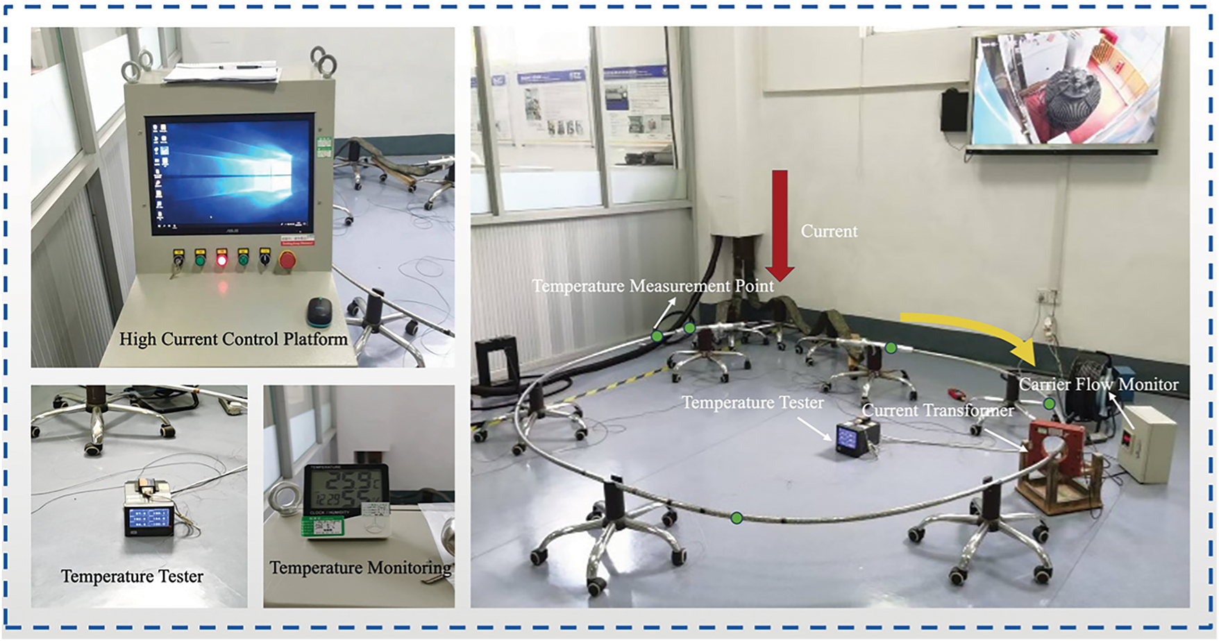
Figure 7: Field construction diagram of experimental platform

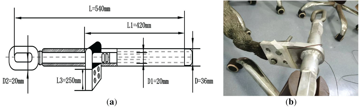
Figure 8: Experimental Apparatus. (a) structural schematic diagram; (b) experimental connection diagram

As summarized in Table 2, the test conductor is an aluminum-clad, steel-reinforced, heat-resistant aluminum alloy wire. To accommodate laboratory constraints, the conductor length was limited to 5 m. Both conductor ends were crimped and secured in accordance with GB/T 32505-2016 (“General Specifications for Wire and Cable Crimping Tools”). The strain clamp was attached to a bus bar, and the aluminum-based crimp tube increased the mass, heat capacity, and heat dissipation area at the connection, inducing axial temperature gradients near the crimp. Five thermocouples were affixed tightly to the conductor and clamp surfaces at points T0–T4 (Fig. 9) to record temperature. Two thermocouples were placed on the clamp surface and three on the conductor surface.

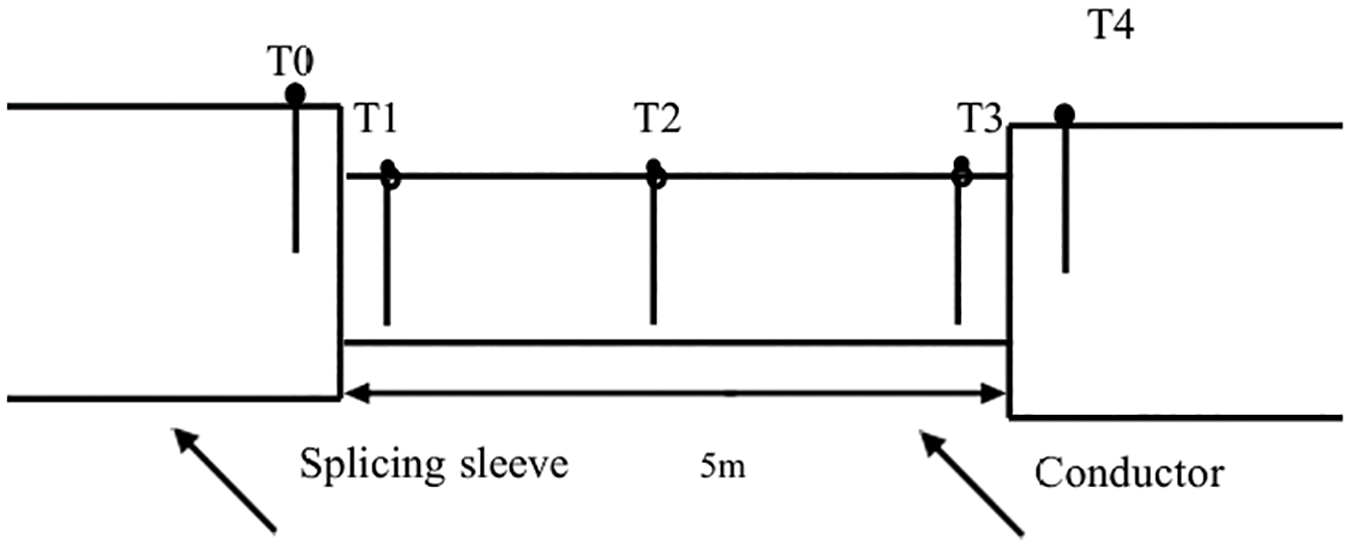
Figure 9: Schematic diagram of temperature measurement points

5.2 Experimental Procedure

To characterize temperature-rise behavior in the clamp-conductor interface, a series of steady-state experiments were performed. Conductor currents of 400, 500, 700, 800, and 1000 A were applied in separate trials. Surface temperatures at the clamp and along the conductor were measured every 5 min until thermal equilibrium, and stabilization times were recorded. Ambient chamber temperature was held at 25°C throughout the tests. The detailed experimental procedure is as follows:

A continuous current of 400 A was applied to the conductor, and the temperatures at designated measurement points were recorded at 5-min intervals over a duration of 75 min, until a thermal steady state was reached. It was observed that the temperature of the splice clamp stabilized at approximately 28.9°C after around 30 min, which is well below the maximum allowable operating temperature of 70°C for the clamp. This indicates that under a 400 A load, the conductor generates only minimal heat and exhibits considerable dynamic overload capacity, suggesting that the current can be moderately increased without driving the temperature to hazardous levels.

Subsequently, a continuous current of 500 A was applied under identical conditions, with temperatures recorded every 5 min for 75 min. The clamp temperature stabilized at 31.2°C after approximately 30 min. The rate of temperature rise was only marginally higher than at 400 A, and the steady-state temperature remained far below the maximum allowable threshold of 70°C. This further confirms that the conductor retains significant dynamic thermal margin at 500 A, allowing for safe current increases under controlled conditions.

With a continuous current of 700 A, temperature measurements were again recorded at 5-min intervals for 75 min. The clamp temperature stabilized at 45.0°C after approximately 70 min. Compared to the 400 A condition, the temperature rise was noticeably faster, indicating a reduction in dynamic overload capacity. Nevertheless, a moderate short-term current increase remains feasible, provided that real-time temperature remains below the clamp’s rated thermal limit.

Finally, at a sustained current of 800 A, the conductor was monitored under the same procedure. The temperature reached a steady value of 53.9°C after approximately 70 min. At this level, the temperature rises more rapidly than at lower current levels, signifying a further decline in dynamic overload tolerance. In practical engineering applications, any additional increase in current beyond 800 A should be approached with caution, and more frequent or continuous temperature monitoring is recommended to ensure operational safety.

At 1000 A—the conductor’s maximum load capacity—there is virtually no margin for dynamic over-load. Any increase beyond this level must be limited to brief emergency adjustments.

Table 3 summarizes the temperature differences between measurement points on the splice clamp and the conductor. It is evident that the maximum temperature difference increases as the load current rises. For example, at 400 A, the maximum axial temperature difference between the splice clamp and the conductor is 33°C. When the current exceeds the conductor’s rated capacity—for instance, at 1000 A—the maximum temperature difference exceeds 70°C. This indicates that the axial temperature gradient at the splice clamp-conductor interface is non-negligible and should be considered in thermal analysis.

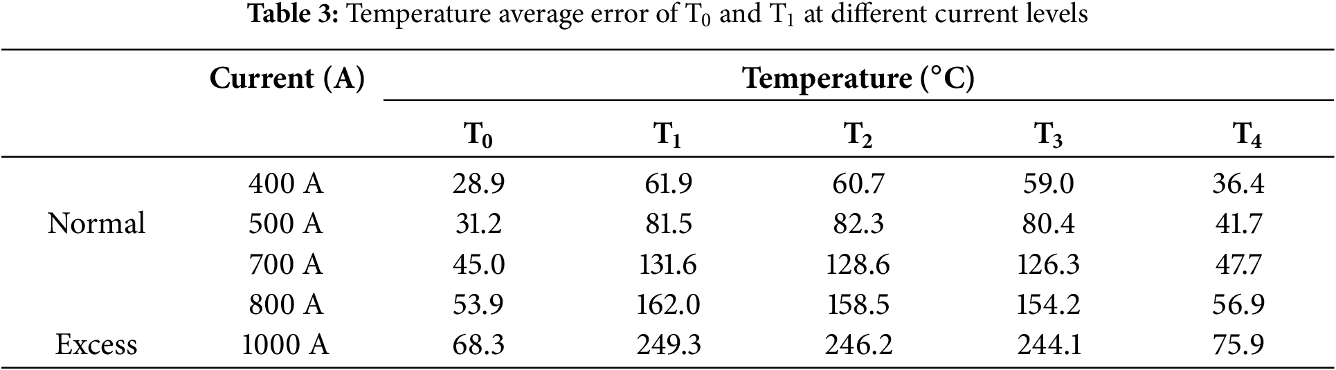
Fig. 10a shows the measured temperature distribution of the splice clamp and conductor under a 400 A load current. The temperature at each measurement point gradually increases and eventually stabilizes at a steady-state value. Notably, the temperature rise of the splice clamp occurs at a relatively slower rate. A similar temperature distribution pattern was observed at other load current levels. Fig. 10b illustrates the simulated temperature evolution at measurement point T0 in the splice clamp–conductor interface under various current loads. If the temperature at the weakest point remains within a safe range after increasing the current load, it indicates that the conductor possesses a certain degree of overload tolerance.

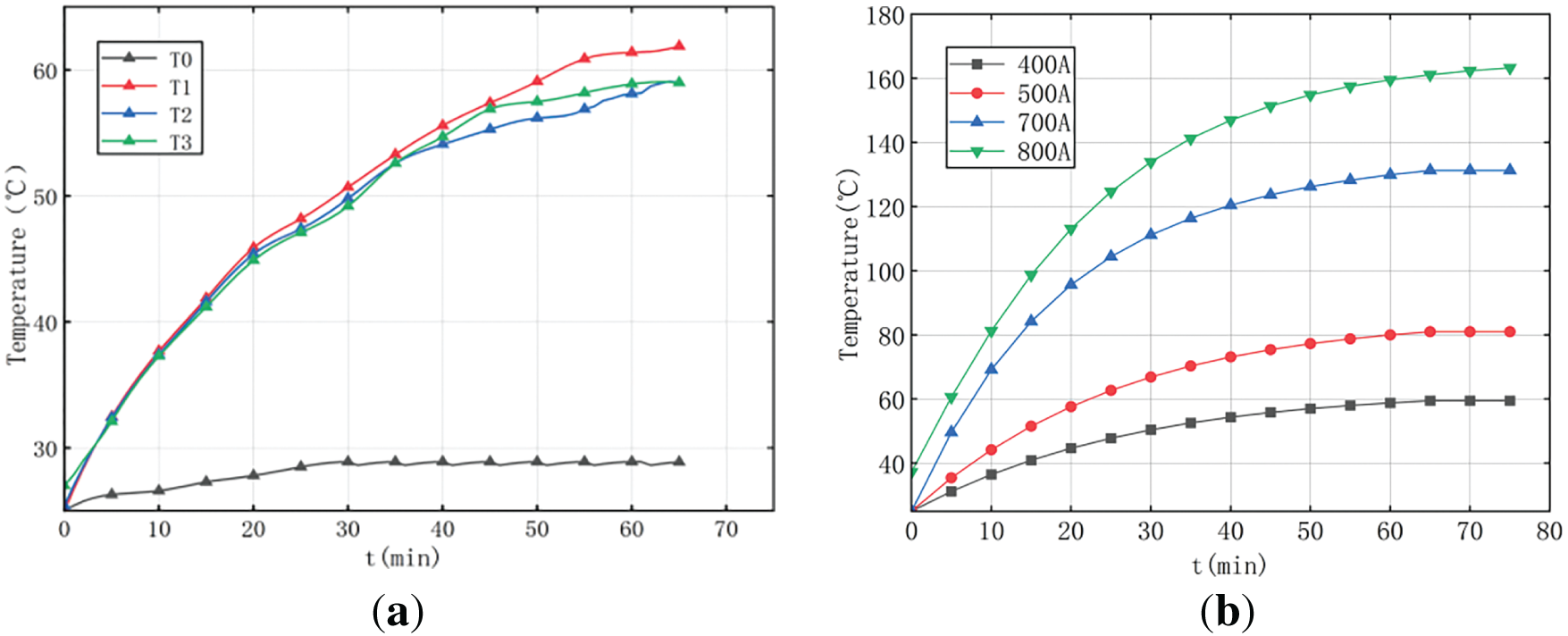
Figure 10: Measured temperature distribution of the conductor with a current of 400 A. (a) 400 A temperature measurement points. (b) T0 measurement point at different current

In addition, a current gradient test was conducted. The conductor was initially allowed to rest in a zero-current state, during which forced convection cooling was applied using a fan to ensure that the initial temperature was consistent with the ambient temperature. Subsequently, a stepwise current-loading protocol was implemented. The conductor was first subjected to an initial current of 850 A, which was held constant for approximately 30 min until thermal stabilization occurred. The current was then increased in increments of 50 A, with the system allowed to reach thermal equilibrium at each current level before proceeding to the next step, until a maximum current of 1000 A was reached. Once the current reached 1000 A, it was maintained until the temperature again reached a stable state. The steady-state temperature distribution under each current gradient is shown in Table 4, The final steady-state temperature achieved under this gradual current ramping process was compared with the steady-state temperature obtained under direct application of 1000 A, in order to assess the thermal response characteristics and potential hysteresis effects of the conductor system.

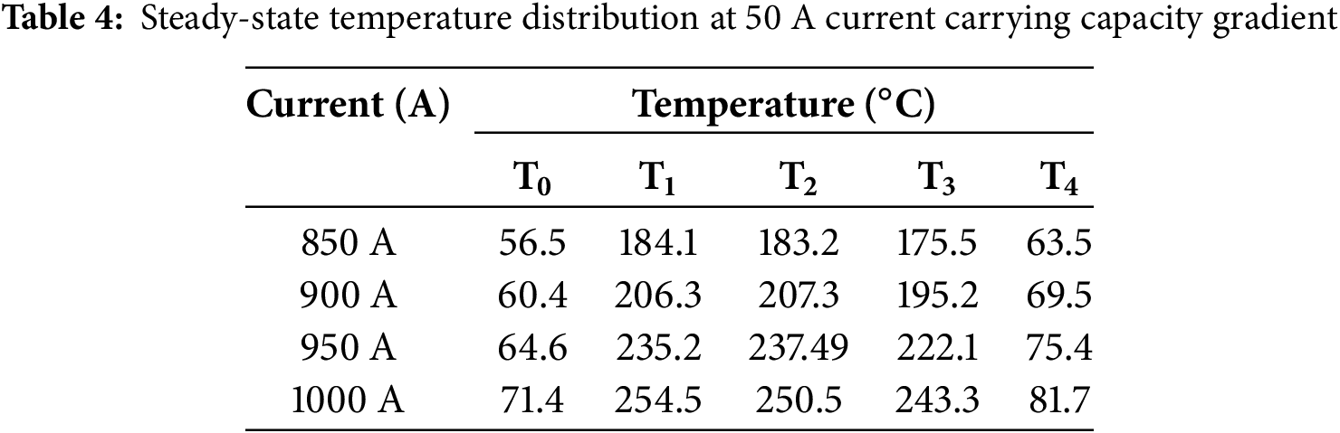
The experimental results show that the time required to reach the steady-state temperature is longer with a 50 A gradient loading compared to directly loading to 1000 A, and the steady-state temperature is higher when gradient loading to 1000 A. The reason may be that the gradient heating causes the wire to preheat, resulting in increased resistance and more heat generation.

5.3 Parameter Identification Validation

The model parameters were identified using the measured temperatures of the splice clamp and conductor. The identified parameters are listed in Table 5. Figs. 11–14 show the trend of the identification parameters under current carrying capacities of 400, 500, 700, and 800 A, respectively.

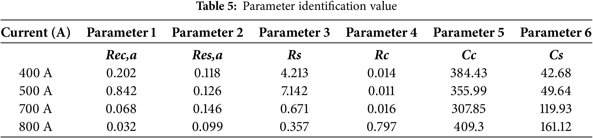
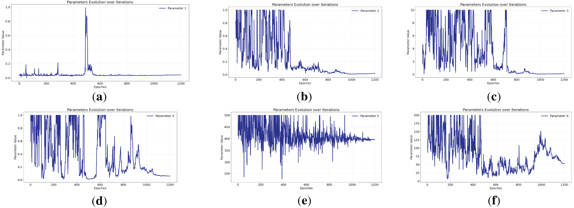
Figure 11: 400 A Parameter Identification Trend Chart. (a) 400 Parameter 1—a in the formula for thermal resistance between conductor and environment; (b) 400 Parameter 2—a in the formula for thermal resistance between conductor and environment; (c) 400 Parameter 3—conductive thermal resistance between clamp microelements; (d) 400 Parameter 4—conductive thermal resistance between wire elements; (e) 400 Parameter 5—conductor thermal capacity; (f) 400 Parameter 6—clamp thermal capacity

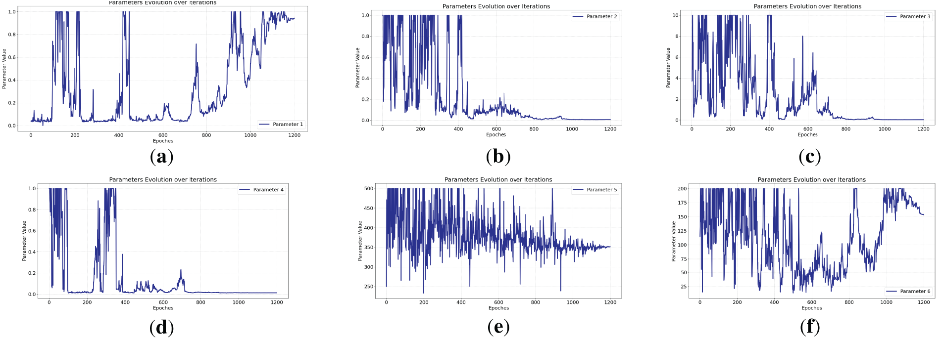
Figure 12: 500 A Parameter Identification Trend Chart. (a) 500 Parameter 1—a in the formula for thermal resistance between conductor and environment; (b) 500 Parameter 2—a in the formula for thermal resistance between conductor and environment; (c) 500 Parameter 3—conductive thermal resistance between clamp microelements; (d) 500 Parameter 4—conductive thermal resistance between wire elements; (e) 500 Parameter 5—conductor thermal capacity; (f) 500 Parameter 6—clamp thermal capacity

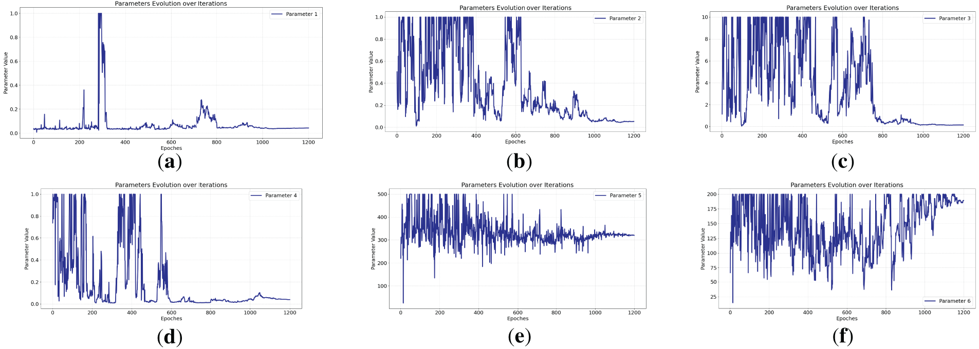
Figure 13: 700 A Parameter Identification Trend Chart. (a) 700 Parameter 1—a in the formula for thermal resistance between conductor and environment; (b) 700 Parameter 2—a in the formula for thermal resistance between conductor and environment; (c) 700 Parameter 3—conductive thermal resistance between clamp microelements; (d) 700 Parameter 4—conductive thermal resistance between wire elements; (e) 700 Parameter 5—conductor thermal capacity; (f) 700 Parameter 6—clamp thermal capacity

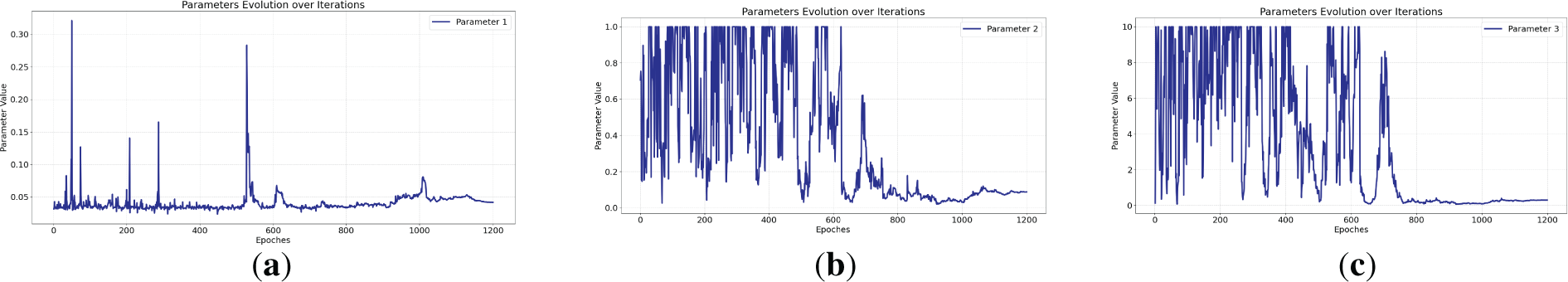
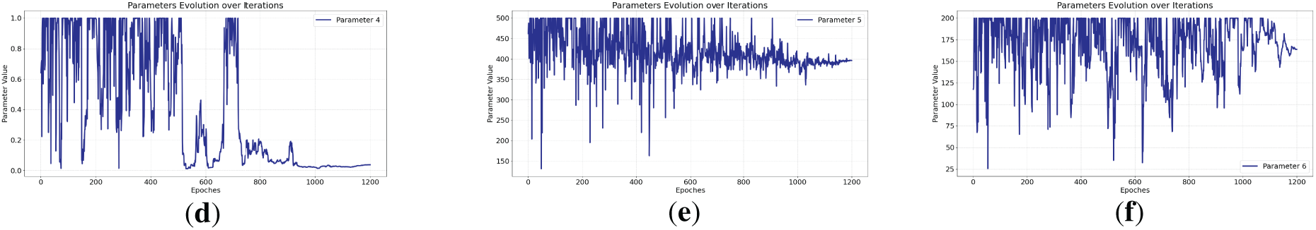
Figure 14: 800 A Parameter Identification Trend Chart. (a) 800 Parameter 1—a in the formula for thermal resistance between conductor and environment; (b) 800 Parameter 2—a in the formula for thermal resistance between conductor and environment; (c) 800 Parameter 3—conductive thermal resistance between clamp microelements; (d) 800 Parameter 4—conductive thermal resistance between wire elements; (e) 800 Parameter 5—conductor thermal capacity; (f) 800 Parameter 6—clamp thermal capacity

Experimental procedures and parameter set Based on prior knowledge and a series of test experiments, all experiments in this paper were conducted with a population size of 80 and 1200 iterations. This ensures more accurate experimental results while also demonstrating the versatility and fairness of the experimental parameters. In the experimental procedure, we conducted two experiments for each set of data. In the first experiment, we first assigned broad upper and lower threshold values to the six parameters to be identified, with the thresholds being (0, 50), (0, 50), (0, 10), (0, 10), (0, 500), and (0, 200). These thresholds were referenced from a large number of articles in the field and are highly persuasive. In the second experiment, based on the parameter identification results from the first experiment, the upper and lower limits of the parameters were further narrowed.

Figs. 11–14 show the trend diagrams of the identified parameters under current ratings of 400, 500, 700, and 800 A, respectively. It can be observed that after the initial random initialization of all parameters, subsequent iterations resulted in varying degrees of fluctuation in the parameters. However, after controlling their upper and lower limits and undergoing algorithmic iterations, the parameters eventually stabilized. As shown in Table 5, the six identification parameters across the four experiments are largely within the same range with minimal differences, further validating the effectiveness and broad applicability of the proposed temperature rise model equation.

Table 6 summarizes average computational errors for conductor temperatures at various load currents, with the maximum mean error not exceeding 1.4%. These findings demonstrate the model’s high accuracy in capturing the temperature rise dynamics of conductors equipped with splice clamps.

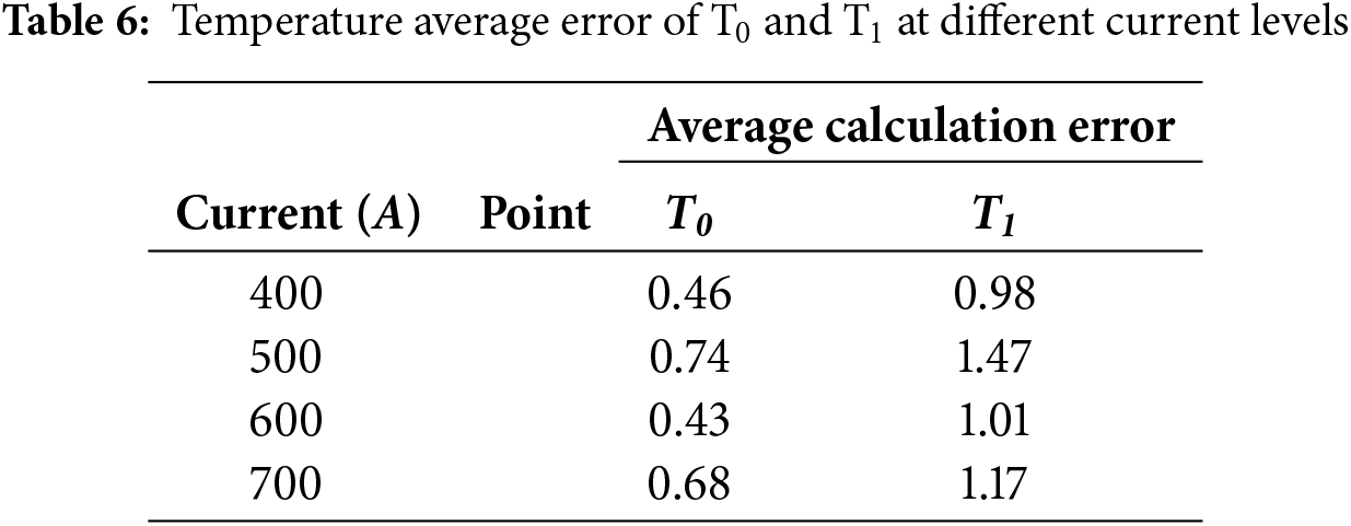
Fig. 15 shows the simulated temperature rise curves and actual measurement curves of the line clamp conductors under 400, 500, 700, and 800 A. It can be seen that the fitting results are good. For the smooth experimental data curves, the simulated curves basically coincide with them, proving the validity of the proposed temperature rise model formula. The temperature rise curves for conductors at 400 and 800 A exhibit significant fluctuations and are not smooth, but the simulated curves still demonstrate strong fitting capability overall.

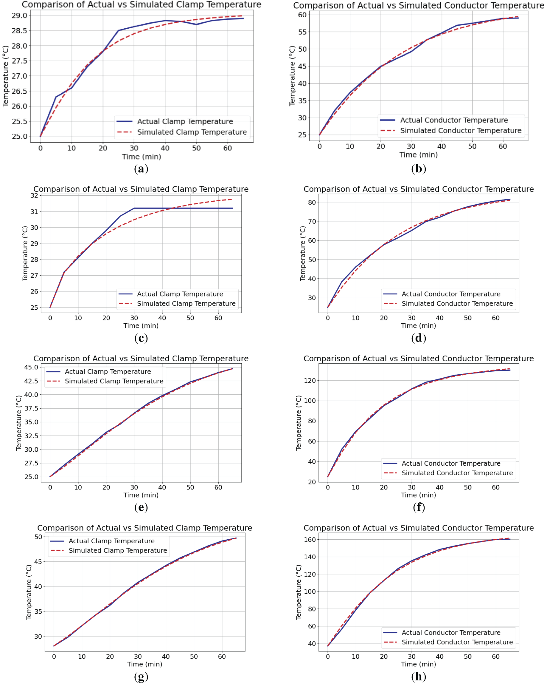
Figure 15: Actual vs Simulated clamp and conductor at different current. (a) T0 temperature Comparison of 400 A; (b) T1 temperature Comparison of 400 A; (c) T0 temperature Comparison of 500 A; (d) T1 temperature Comparison of 500 A; (e) T0 temperature Comparison of 700 A; (f) T1 temperature Comparison of 700 A; (g) T0 temperature Comparison of 800 A; (h) T1 temperature Comparison of 800 A

Fig. 16 shows computed temperatures at points T0 and T1 under various load currents. Fig. 17 shows the calculation errors of conductors and clamps at different current levels. It can be seen that under different current carrying capacities, the maximum temperature difference error of the clamps reaches 2.79%, and the maximum temperature difference error of the conductors reaches 2.01%.

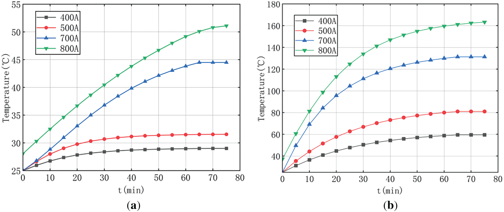
Figure 16: Calculated temperature of conductor and clamp at different current levels. (a) T0 Calculated temperature. (b) T1 Calculated temperature

Figure 17: Calculation error of the conductor and clamp at different current levels. (a) T0 Calculation error. (b) T1 Calculation error

6  Conclusions

This paper builds upon existing research, moving from a single consideration of clamp temperature rise or conductor temperature rise to proposing an axial heat transfer model for clamps and conductors. It employs the WOA parameter identification method to predict temperature rise in the conductor-clamp coupling zone. Experimental verification demonstrates that the WOA parameter identification method achieves good accuracy,the six identification parameters across the four experiments are largely within the same range with minimal differences. The identified parameters were entered into the temperature rise model for calculation, and it was found that the model could accurately predict the temperature distribution at the interface between the clamp conductor and the adjacent conductor segment under natural convection conditions, with a maximum error of only 2.79%. This demonstrates that the model is effective in predicting the temperature in the clamp-conductor coupling zone.

Moreover, this work establishes a robust foundation for accurate temperature prediction in clamp-conductor interfaces under real world meteorological conditions and supports dynamic capacity enhancement of overhead conductors. Future efforts will focus on algorithm enhancement, as well as considering the impact of various coupling factors on conductor temperature rise.

Key conclusions:

(1)   The method based on WOA parameter identification can accurately identify thermal parameters and solve the problem of determining model parameters. According to the experimental results, under different load currents, the maximum temperature difference of the line clamp reached 2.79%, the maximum temperature difference of the conductor reached 2.01%, and the maximum average error did not exceed 1.4%, effectively verifying the feasibility of the WOA parameter identification method.

(2)   This paper draws clear conclusions regarding the modeling of temperature distribution in the clamp-conductor coupling zone. The thermal model established, which takes into account axial heat transfer between the clamp and conductor, is effective in predicting the temperature at the clamp-conductor interface.

Acknowledgement: Not applicable.

Funding Statement: (1) This work was supported by the Technology Innovation Leading Program of Shaanxi (2024QCY-KXJ-009) and the Research Plan of the Education Department of Shaanxi Province (23JC028). (2) This work was supported by the National Key Laboratory of Metal Forming Technology and Heavy Equipment B2408100.W14. (3) Key Research and Development Program of Shaanxi (2025CY-YBXM-489).

Author Contributions: The authors confirm contribution to the paper as follows: Conceptualization, Long Zhao; methodology, Long Zhao; validation, Long Zhao, Qi Zhao and Siyuan Zhou; formal analysis, Qi Zhao; investigation, Siyuan Zhou; resources, Long Zhao; data curation, Chao Ji; writing—original draft preparation, Long Zhao; writing—review and editing, Long Zhao and Qi Zhao; visualization, Siyuan Zhou; review, edit and visualize, Chenyang Fan; supervision, Chao Ji; project administration, Long Zhao; funding acquisition, Long Zhao. All authors reviewed the results and approved the final version of the manuscript.

Availability of Data and Materials: Not applicable.

Ethics Approval: Not applicable.

Conflicts of Interest: The authors declare no conflicts of interest to report regarding the present study.

Abbreviation

References

1. Cecchi V, Knudson M, Miu K. System impacts of temperature-dependent transmission line models. IEEE Trans Power Deliv. 2013;28(4):2300–8. doi:10.1109/TPWRD.2013.2276757. [Google Scholar] [CrossRef]

2. Conseil International des Grands Réseaux Électriques. Comité d′études B2. Guide for qualifying high temperature conductors for use on overhead transmission lines. In: Proceedings of the CIGR; 2010 Jun 13–17; Québec City, QC, Canada. [Google Scholar]

3. Foss SD, Lin SH, Fernandes RA. Dynamic thermal line ratings part I dynamic ampacity rating algorithm. IEEE Trans Power Apparatus Syst. 1983;PAS-102(6):1858–64. doi:10.1109/TPAS.1983.317795. [Google Scholar] [CrossRef]

4. Craven GT, Nitzan A. Electrothermal transistor effect and cyclic electronic currents in multithermal charge transfer networks. Phys Rev Lett. 2017;118(20):207201. doi:10.1103/PhysRevLett.118.207201. [Google Scholar] [PubMed] [CrossRef]

5. Sun WQ, Zhang Y, Wang CM, Song P. Flexible load shedding strategy considering real-time dynamic thermal line rating. IET Gener Transm Distrib. 2013;7(2):130–7. doi:10.1049/iet-gtd.2012.0117. [Google Scholar] [CrossRef]

6. Matsushita T, Belov I, Johansson A, Jarfors AEW. Influence of contact pressure on the thermal contact conductance of layered metallic sheets. High Temp High Press. 2022;51(1):63–82. doi:10.32908/hthp.v51.1107. [Google Scholar] [CrossRef]

7. Azevedo CRF, Cescon T. Failure analysis of aluminum cable steel reinforced (ACSR) conductor of the transmission line crossing the Paraná River. Eng Fail Anal. 2002;9(6):645–64. doi:10.1016/S1350-6307(02)00021-3. [Google Scholar] [CrossRef]

8. Dong XC, Qu FR, Li YF, Wang YQ. Simulation analysis and verification on three-dimensional temperature field of strain clamps for overhead lines. J Southwest Jiaotong Univ. 2019;54(5):997–1004. doi:10.3969/j.issn.0258-2724.20180610. [Google Scholar] [CrossRef]

9. Lin J, Liu G, Zhang H, Sun J. Research of temperature distribution of overhead lines parallel groove clamp. Power Syst Prot Control. 2013;41(24):88–94. (In Chinese). [Google Scholar]

10. Angadi SV, Jackson RL, Pujar V, Tushar MR. A comprehensive review of the finite element modeling of electrical connectors including their contacts. IEEE Trans Compon Packag Manuf Technol. 2020;10(5):836–44. doi:10.1109/TCPMT.2020.2982207. [Google Scholar] [CrossRef]

11. Zhang J, Yang B, Sun H, Zhou Y, Liu M, Ding J, et al. Aquaporin-4 deficiency diminishes the differential degeneration of midbrain dopaminergic neurons in experimental Parkinson’s disease. Neurosci Lett. 2016;614(Pt 5):7–15. doi:10.1016/j.neulet.2015.12.057. [Google Scholar] [PubMed] [CrossRef]

12. He W, Feng Y, Wu S, Wang W. Mechanical-thermal–electrical coupling modeling and temperature rise characteristic of a parallel groove clamp with improved representation of contact interactions. IEEE Trans Compon Packag Manuf Technol. 2023;13(3):356–64. doi:10.1109/TCPMT.2023.3263471. [Google Scholar] [CrossRef]

13. Zhang J, Zhang Z, Si J, Liu P. Research on temperature rise characteristics and resistance changes of typical contact fittings. In: 2023 IEEE International Conference on Sensors, Electronics and Computer Engineering (ICSECE); 2023 Aug 18–20; Jinzhou, China. p. 1638–43. doi:10.1109/ICSECE58870.2023.10263312. [Google Scholar] [CrossRef]

14. Huang W. Temperature rise characteristics and life prediction of corroded parallel groove wire clamps [master’s thesis]. Chongqing, China: Chongqing University; 2023. (In Chinese). [Google Scholar]

15. Liao Y, Jiang XL, Zhao JC, Zhang ZJ, Huang WH. Study on temperature rise characteristics and feature quantity of galvanized clamps for atmospheric corrosion. Trans China Electrotech Soc. 2024;39(23):7592–604. (In Chinese). doi:10.19595/j.cnki.1000-6753.tces.231464. [Google Scholar] [CrossRef]

16. Tan Z, Chen S, Guan W, Guo J. Thermal-electric-structure coupling finite element analysis and experimental study of AgNi10 contact material under the closed contact stage. Rare Met Mater Eng. 2012;41(2):276–80. [Google Scholar]

17. Bühlmann P, Meier M, Vifian M, Mazza E, Franck C. Temperature profile along an overhead line conductor in and near the tension clamp. In: Proceedings of the CIGRE Session; 2016 Aug 21–26; Paris, France. [Google Scholar]

18. Bühlmann P, Franck C. Temperature profiles of all-aluminum-alloy conductors near wedge tension clamps. CIGRE Sci Eng. 2018;10:66–76. [Google Scholar]

19. Dong X, Qu F, Li Y, Fang B, Wang Y, Liu G. Experimental analysis of temperature distribution in high-voltage strain clamp. In: 2018 12th International Conference on the Properties and Applications of Dielectric Materials (ICPADM); 2018 May 20–24; Xi’an, China. p. 829–32. doi:10.1109/ICPADM.2018.8401157. [Google Scholar] [CrossRef]

20. Beloufa A. The effect of cable section on the variation of power automotive connector temperature. IEEE Trans Compon Packag Manuf Technol. 2019;9(6):1020–8. doi:10.1109/TCPMT.2019.2914894. [Google Scholar] [CrossRef]

21. Soppe B, Frehn T, Puffer R, Krispin HJ, Dansachmueller M, Zemke S. Thermal modelling of fittings for high temperature low sag conductors. In: Proceedings of the VDE High Voltage Technology 2020, ETG-Symposium; 2020 Nov 9–11; Online. p. 1–17. [Google Scholar]

22. Jin Y, Quan M, Yan S, Yan Y, Cui M, Liu Y. Analysis of overhead transmission lines fusing failure due to poor contact between conductors and clamps. Eng Fail Anal. 2020;118:104858. doi:10.1016/j.engfailanal.2020.104858. [Google Scholar] [CrossRef]

23. Yang X, Tu Y, Yuan Z, Zheng Z, Chen G, Wang C, et al. Intelligent overheating fault diagnosis for overhead transmission line using semantic segmentation. High Volt. 2024;9(2):309–18. doi:10.1049/hve2.12403. [Google Scholar] [CrossRef]

24. Wang Y, Miao H, Mo ST, Zha YF, Li RJ. Analysis of heat transfer of ice-melted steel core aluminum insulated wire. Electr Meas Instrum. 2024;61(1):59–63. (In Chinese). doi:10.19753/j.issn1001-1390.2024.01.009. [Google Scholar] [CrossRef]

25. Zhou Y, Hao S, Qi W. Radial temperature field analysis of long-span transmission wires considering turbulent flow. Environ Technol. 2024;42:29–35. (In Chinese). [Google Scholar]

26. Black WZ, Collins SS, Hall JF. Theoretical model for temperature gradients within bare overhead conductors. IEEE Trans Power Deliv. 1988;3(2):707–15. doi:10.1109/61.4309. [Google Scholar] [CrossRef]

27. Hou Y, Wang W, Wei Z, Deng X, Ji Q, Wang T, et al. Research and application of dynamic line rating technology. Energy Rep. 2020;6(2):716–30. doi:10.1016/j.egyr.2020.11.140. [Google Scholar] [CrossRef]

28. Dai YJ, Ren XJ, Wang YG, Xiao Q, Tao WQ. Effect of thermal expansion on thermal contact resistance prediction based on the dual-iterative thermal-mechanical coupling method. Int J Heat Mass Transf. 2021;173(2):121243. doi:10.1016/j.ijheatmasstransfer.2021.121243. [Google Scholar] [CrossRef]

29. Kweon D, Koo K, Woo J, Kim Y. Hot spot temperature for 154 kV transformer filled with mineral oil and natural ester fluid. IEEE Trans Dielectr Electr Insul. 2012;19(3):1013–20. doi:10.1109/TDEI.2012.6215107. [Google Scholar] [CrossRef]

30. Zhang X, Ying Z, Chen Y, Chen X. A thermal model for calculating axial temperature distribution of overhead conductor under laboratory conditions. Electr Power Syst Res. 2019;166(2):223–31. doi:10.1016/j.epsr.2018.10.008. [Google Scholar] [CrossRef]

31. Hu J, Xiong XF, Wang J. Radial and circumferential temperature calculation method of overhead transmission lines based on thermal network model. Trans China Electrotech Soc. 2019;34(1):139–52. (In Chinese). doi:10.19595/j.cnki.1000-6753.tces.180398. [Google Scholar] [CrossRef]

32. Luo D, Wang T, Han J, Niu D. Study of three-dimensional distribution of chloride in coral aggregate concrete: a CNN-BiGRU-attention data-intelligence model driven by Beluga whale optimization algorithm. Constr Build Mater. 2025;458(4):139740. doi:10.1016/j.conbuildmat.2024.139740. [Google Scholar] [CrossRef]

33. He W, Feng Y, Wu S, Wu K, Wang W. Effect of elastoplastic thermal softening on thermal contact resistance based on the dual-load transfer coupling method. Int J Therm Sci. 2023;183(6):107835. doi:10.1016/j.ijthermalsci.2022.107835. [Google Scholar] [CrossRef]