
 Submit a Paper
 Propose a Special lssue
 Open Access
ARTICLE

Methods of Selecting Adaptive Artificial Viscosity in Completely Conservative Difference Schemes for Gas Dynamics Equations in Euler Variables
1 Keldysh Institute of Applied Mathematics of Russian Academy of Sciences, Moscow, 125047, Russia
2 Department of Mathematical Modeling and Applied Mathematics, Phystech School of Applied Mathematics and Computer Science, Moscow Institute of Physics and Technology (National Research University), Dolgoprudny, 141701, Russia
* Corresponding Author: Viktoriia Podryga. Email:
(This article belongs to the Special Issue: Heat and Mass Transfer in Energy Equipment)
Frontiers in Heat and Mass Transfer 2025, 23(6), 1789-1809. https://doi.org/10.32604/fhmt.2025.066953
Received 21 April 2025; Accepted 30 July 2025; Issue published 31 December 2025
 View Full Text
 Download PDF
Abstract
The work presents new methods for selecting adaptive artificial viscosity (AAV) in iterative algorithms of completely conservative difference schemes (CCDS) used to solve gas dynamics equations in Euler variables. These methods allow to effectively suppress oscillations, including in velocity profiles, as well as computational instabilities in modeling gas-dynamic processes described by hyperbolic equations. The methods can be applied both in explicit and implicit (method of separate sweeps) iterative processes in numerical modeling of gas dynamics in the presence of heat and mass transfer, as well as in solving problems of magnetohydrodynamics and computational astrophysics. In order to avoid loss of solution accuracy on spatially non-uniform grids, in this work an algorithm of grid embeddings is developed, which is applied near transition points between cells of different sizes. The developed algorithms of CCDS using the methods for AAV selection and the algorithm of grid embeddings are implemented for various iterative processes. Calculations are performed for the classical problem of decay of an arbitrary discontinuity (Sod’s problem) and the problem of propagation of two symmetric rarefaction waves in opposite directions (Einfeldt’s problem). In the case of using different methods for selecting the AAV, a comparison of the solutions of the Sod’s problem on uniform and non-uniform grids and a comparison of the solutions of the Einfeldt’s problem on a uniform grid are performed. As a result of the comparative analysis, the applicability of these methods is shown in the spatially one-dimensional case (explicit and implicit iterative processes). The obtained results are compared with the data from the literature. The results coincide with analytical solutions with high accuracy, where the relative error does not exceed 0.1%, which demonstrates the effectiveness of the developed algorithms and methods.Keywords
The gas dynamics equations are the expressions of the basic conservation laws (mass, momentum, and energy) in a continuous medium. Therefore, it is natural to construct a discrete model of the medium under study in such a way that the discrete analogues for these laws are also fulfilled in it. Practice shows that the application of such difference schemes is especially effective for solving the problems in which solution profiles change sharply in time and space. Further developing the integral consistency principles for the mass, momentum, and various types of energies led to the completely conservative difference schemes (CCDS) [1], which discretely conserve also the internal and kinetic energies of the system and are used in Lagrangian and Eulerian methods of describing the continuous medium [2–4]. Introducing the adaptive artificial viscosity (AAV) [5] into the CCDS allows to suppress the oscillations arising in the numerical solution locally. It is made by controlling the spatial approximation of the discrete model without changing its properties of conservative consistencies by the various types of energy, mass transfer and momentum components. In this case, a qualitative physical solution of the problem is obtained. The solution of the nonlinear algebraic equations system corresponding to the implicit CCDS is realized by some iterative process. Note also that the different iterative processes used in this work affect the choice of the AAV type in the difference scheme and thus determine the dynamically generated local approximation of this difference scheme.
In the last years, the introduction of the AAV is a widely used method for suppressing the computational instabilities arising in discrete modelling of transport processes in the mathematical physics problems [6–18]. In work [6], a method of the global AAV by space for the conservative laws was developed, but it was required to refine the AAV coefficient on a coarse grid, then perform the calculation on a fine grid. In work [7], a new method for constructing the adaptive artificial viscosity in the context of one-dimensional, staggered-grid Lagrangian hydrodynamics, was proposed to accurately model the non-viscous flow with the shock wave. In work [8], a wave number based on the AAV addition method for quintic spline reconstruction scheme was studied for flows with discontinuities and a broad range of scales, e.g., shock-turbulence interactions. In work [9], the AAV model depending on the smoothness indicator was considered. In work [10], the difference schemes with Lax-Wendroff corrections and the AAV were proposed. In work [11], the corrective mechanism with an entropy-based adaptive artificial viscosity was investigated. In work [12], an entropy-stable artificial viscosity with the production of coefficients for the first-order Graph Viscosity and high-order Graph Viscosity (entropy viscosity) methods was also used for the Euler equations system. In work [13], a provably entropy stable shock capturing approach for the high order entropy stable discontinuous Galerkin spectral element method based on a hybrid blending with a subcell low order variant was studied. The AAV was also used for solving the shallow water flows problem [14], reducing grid orientation effect in numerical modelling for steam thermal recovery [15], modelling the two-phase flow in porous media [16] and modelling the atmosphere dynamics process [17]. This work presents the methods for selecting the local AAV that is automatically tuned in the iterative processes.
The present study is a continuation of the work [19]. In work [19], a calculation of artificial viscosity coefficients was an internal iterative process at each iteration of the sweep algorithm. In the present work, some realisations of the CCDS with the AAV using the different iterative processes are proposed. We present the method of the explicit iterations, the method of the sweep algorithm with a one-time change of the artificial viscosity coefficients at one iteration and the improved method of the explicit iterations, which are used to solve the problem of arbitrary discontinuity decay (Sod’s problem [20]) and the problem of two symmetric rarefaction waves propagation in the opposite directions (Einfeldt’s problem [21]). A simple implementation of the developed methods is shown. To solve the Sod’s problem and the Einfeldt’s problem, the methods are implemented using the same algorithms with the same parameters of the AAV selection algorithms. This study also presents the method to incorporating the AAV to effectively suppress the oscillations in the velocity and pressure profiles. A comparative analysis of the developed iterative methods and approaches to the AAV selection is carried out, and their efficiency compared to the works of other authors [6–9,22–24] is shown. This work also proposes the grid embedding method to solve the problem on spatially irregular grids.
Due to the impossibility of applying the sweep method in the spatially multidimensional case on the irregular grids, the improved method of explicit iterations developed in this work can be effectively used to solve such problems.
The Section 2 presents the initial formulation of the gas dynamics problem in Euler variables, a two-layer time-dependent fully conservative difference scheme for its solution and approximation operators for the system of equations in Euler variables. The Section 3 describes the methods and approaches developed and used in this work, which are the method of explicit iterations, the method of joint iterations, the improved method of explicit iterations, the velocity viscosity approach and the grid embedding method. Section 4 demonstrates the computational results obtained by the different methods and gives their comparative analyses.
2 Formulation of the Gas Dynamics Problem in Eulerian Variables
Consider a spatially one-dimensional flow of a compressible gas in Euler variables in the Cartesian coordinate system:
Here
Fig. 1 corresponds to the difference scheme Eqs. (5)–(8). Here
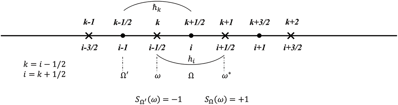
Figure 1: Difference grid. Scheme of grid’s nodes (
Obviously:
where
For the system of Eqs. (1)–(4) we write out the two-layer time completely conservative difference scheme in Euler variables:
where
Quantities from a set of artificial viscosities
On the explicit and implicit time layers
The difference analogues of the vector analysis operations used in Eqs. (5)–(8) and the range and codomain of the corresponding operation analogue are defined as follows:
where
3 Methods for Computing Completely Conservative Difference Schemes
In this work, the improved method of explicit iterations (Section 3.3) based on the method of explicit iterations (Section 3.1) and the method of joint iterations (Section 3.2) are used to realise the nonlinear implicit CCDS. In addition, the velocity viscosity method is used to approximate the velocity (Section 3.4), and the grid embedding method is developed for the problem on a non-uniform grid (Section 3.5).
Hereinafter, all quantities are defined at the nodes except the CFL number and the viscosities (viscous filling
3.1 Method of Explicit Iterations
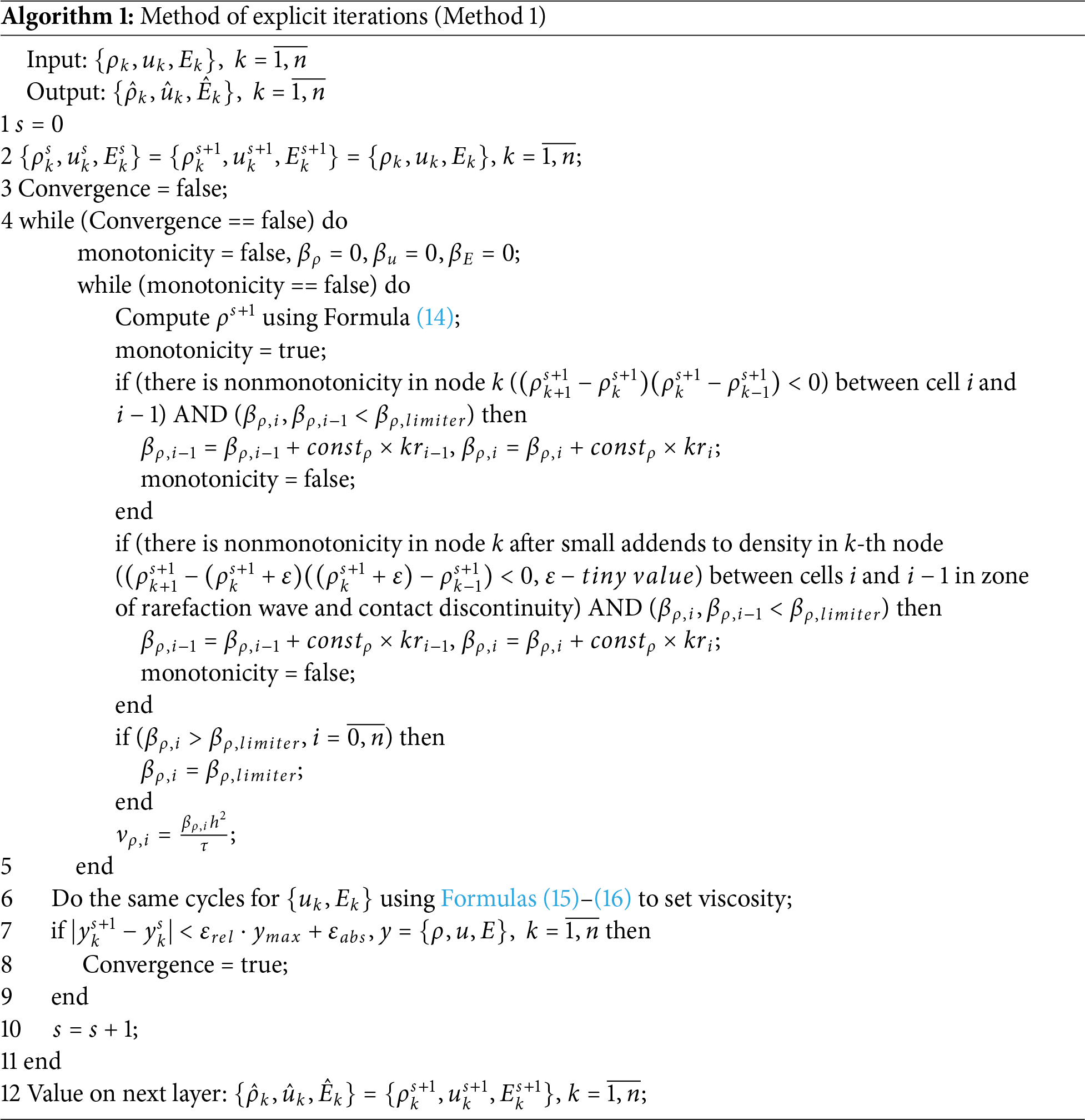
This work presents the explicit iteration method (hereafter Method 1), which also uses additional optimization criteria for the AAV selection in rarefaction wave, shock wave and contact rupture structures, which were tested on solving the Sod’s problem [20]. In the following Sections 3.2 and 3.3, such optimization is not required. Using this method, the satisfactory results are obtained, but the processor time spent on the iterative processes is significant.
In Method 1, an explicit iterative process is performed to calculate the quantities in the next time step. The formulas of this iterative process for the Eqs. (5)–(7) are as follows:
When determining the viscosity in the flux
The algorithm of Method 1 is shown in Algorithm 1.
3.2 Method of Joint Iterations
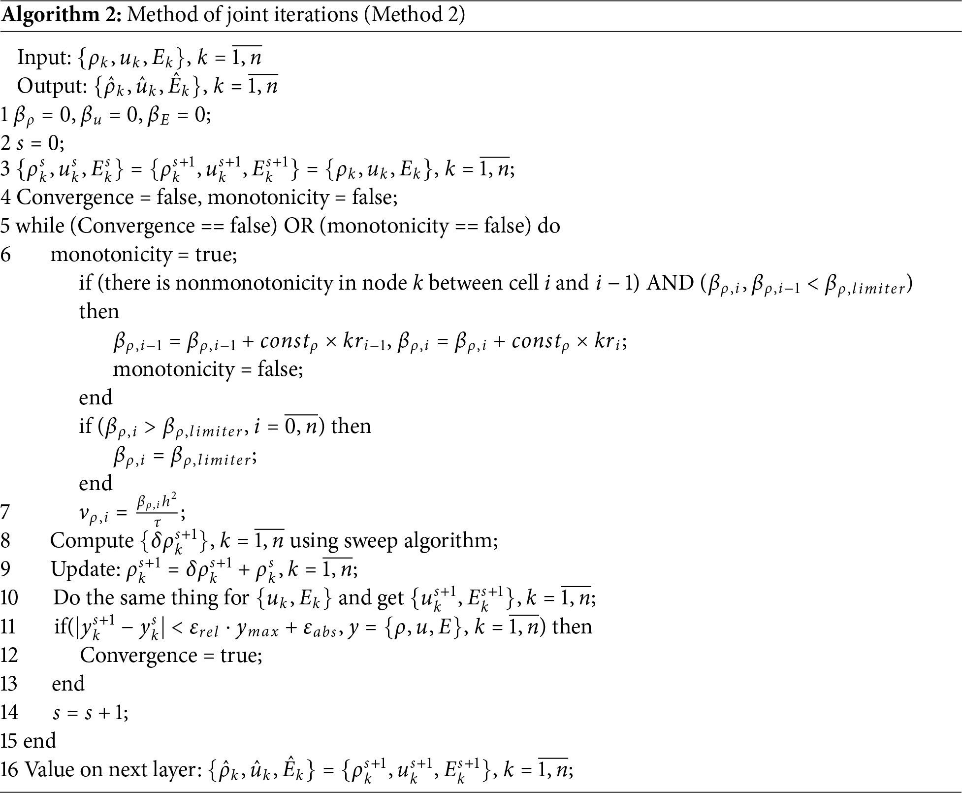
In the current work, in order to optimize the computational process of the CCDS implementation and the AAV selection, we propose the method of joint iterations (hereinafter referred to as Method 2), which simultaneously refines the iterative difference solution and corrects the AAV. Along with Method 1, Method 2 uses the sweep algorithm for the difference balances Eqs. (5)–(7), in which the increments are calculated from the s-th iteration to the
This method is implemented as follows. If oscillations occurred during the computation of
At the beginning of each time step before the iterations begin, all viscosities are assumed to be 0, the values at the first iteration are equal to those at the explicit layer
where
The algorithm of Method 2 is shown in Algorithm 2.
3.3 Improved Method of Explicit Iterations
The efficiency of Method 2, which gives good accuracy in test problems and low processor time, led to a modification of Method 1, increasing its implicit margin (Method 1 is realized by a explicit scheme and explicit iterations). Such an algorithm (hereinafter Method 3) is represented as follows below in the form Algorithm 3, where in the following values are held:
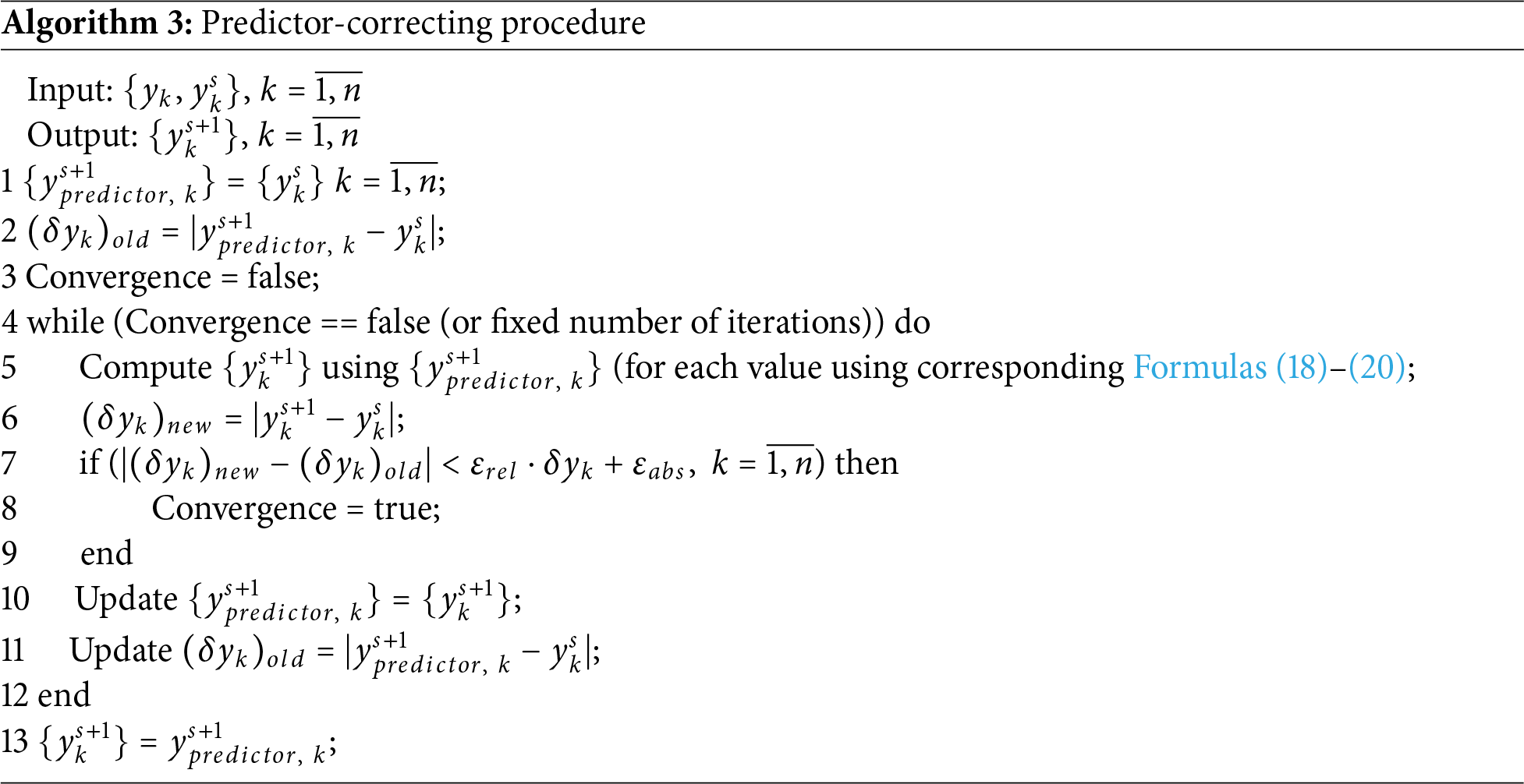
At the
When determining the viscosities in the flux
This process of realizing the solution by explicit iterations introduces an internal iterative process with fixed viscosity. Then, in the presence of oscillations, viscosities are increased and the external iterative process ends when oscillations are corrected and convergence to the solution is available. Algorithm of realization of Method 3 is presented in the form of Algorithm 4.
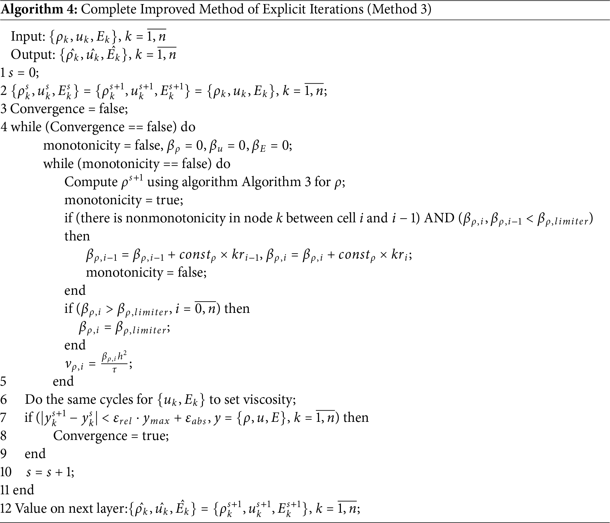
Thus, Method 3 differs from Method 1 by the procedure of calculating at the (
Due to the predictor-correcting procedure, which does not require matrix inversion for a system of algebraic equations in grid space, the implicit scheme is realized by explicit iterations (Method 3). Method 3 in this work is implemented only in the one-dimensional case, but it is possible in two-dimensional and three-dimensional cases, which will be investigated in the future. In Section 4.1.2, it will be shown that Method 3 has higher accuracy than Method 1. In addition, compared to Method 1 calculations, the implicit scheme reduces the convergence time to the solution, although an additional predictor-correcting procedure is performed at each iteration in Method 3.
3.4 Transition from Momentum Viscosity to Velocity Viscosity
When numerically solving by described methods, oscillations in the density and velocity profiles may occur, while oscillations in the momentum profiles are absent. This phenomenon is caused by the momentum viscosity included in
A comparison of the velocity profiles for Method 3 calculations using velocity and momentum viscosity is presented in Fig. 2. The effectiveness of the velocity viscosity in smoothing the oscillations behind the rarefaction wave zone, also in the contact rupture zone, is shown.
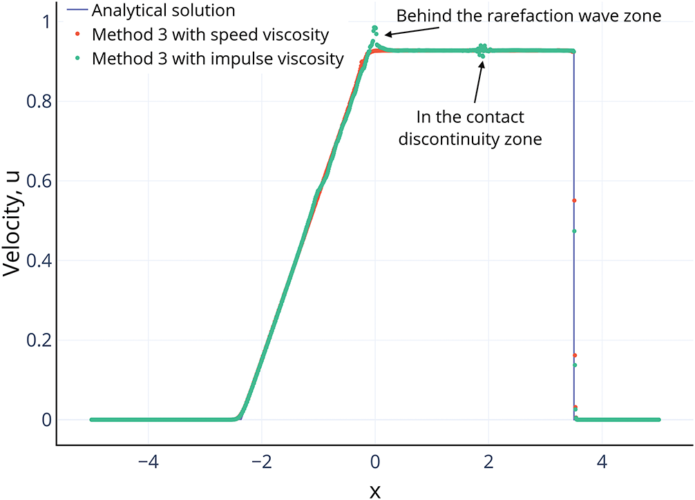
Figure 2: The distribution of over space when solving the Sod’s problem using Method 3 with impulse viscosity (red dots) and with velocity viscosity (green dots) for time
When calculating on spatially non-uniform grid with a significant change in grid sizes, the loss of accuracy of the solution may occur near the point of transition from one grid size to another. In this case, it is proposed to define the values of gas-dynamic quantities not in the initial nodes of the grid, but in the centers of gravity of their nodal domains. To improve the accuracy of calculation on a non-uniform grid, the method of grid embeddings given below is used.
In the zone of break of uniformity of the grid (a node around which two neighboring cells of different lengths), a new node is defined as the center of gravity of two neighboring half-cells. In this way, a new grid (in the case of a uniform grid, completely identical to the original grid), called a centroid with first-order embedding, is generated. For example, for a one-dimensional grid with a change of cell length from 2 to 1 (the irregularity coefficient is 2), after one such embedding the irregularity coefficient of the centroid grid becomes

Figure 3: Example of grid embeddings
4 Numerical Experiments and Analysis of Results
To test the constructed scheme and the developed methods, the Sod’s problem [20] on the decay of an arbitrary discontinuity and the Einfeldt’s problem [21] on the propagation of two symmetric rarefaction waves in opposite directions have been solved.
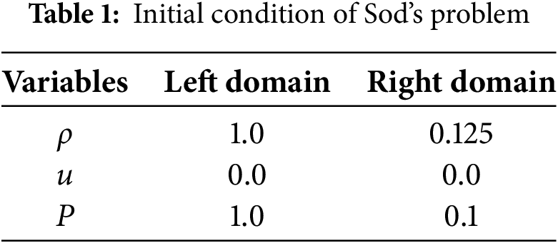
Table 1 shows the initial conditions of the Sod’s problem [20]. The position on the distribution to the left of the center point is the left domain, to the right—the right domain (the center point is included in the right domain). The SI system is taken as the system of units in calculations. Adiabatic index is
The obtained results coincide completely with the results of [5]. In all further calculations,
4.1.1 Calculation Using the Method of Joint Iterations on a Uniform Grid
The density, velocity, pressure, and internal energy distributions are shown in Fig. 4. It can be seen from Fig. 4 that Method 2 improves the results of calculations in the zones of rarefaction wave and contact discontinuity. At the same time, the plots of calculations performed by Method 2 are more close to the analytical solution than the plots of calculations performed by Method 1 in the rarefaction wave zones in all profiles. Also due to the choice of velocity viscosity in the contact discontinuity zone, the oscillations are completely absent in Method 2, while in Method 1 their small amplitude is observed. Method 2 significantly reduces the processor time spent on calculations and more accurately approaches the analytical solution than Method 1. This is due to the implicit nature of finding the increments by the sweep algorithm in the iterative process. Also, in all Method 2 calculations, the viscous limiter

Figure 4: The distributions of (a) density, (b) velocity, (c) pressure, and (d) internal energy over space obtained by solving the Sod’s problem by Method 1 (red line) and Method 2 (green line) for time
4.1.2 Calculation Using the Improved Method of Explicit Iterations on a Uniform Grid
The improved method of explicit iterations (Method 3) does reduce the processor time and number of iterations for convergence compared to Method 1. Fig. 5 shows the distributions of density, velocity, pressure, and internal energy. From Fig. 5, we can see that the accuracy of the solutions in Method 3 is significantly higher (in the sense of convergence to the analytical solution) than in Method 1. Also, no peak in velocity and pressure profiles is observed in the contact discontinuity zone in Method 3. The processor time in Method 3 is an order of magnitude less than in Method 1 and about the same as in Method 2. In Method 3, the limiter

Figure 5: The distributions of (a) density, (b) velocity, (c) pressure, and (d) internal energy over space obtained by solving the Sod’s problem by Method 1 (red line) and Method 3 (green line) for time
4.1.3 Calculation Using the Improved Method of Explicit Iterations on Non-Uniform Grid
Fig. 6 shows the distributions of density, velocity, pressure and internal energy obtained by solving the Sod’s problem using Method 3 on non-uniform and uniform grids. Satisfactory results are observed both without and with the grid embedding method. Although in the two zones the space steps on the non-uniform grid are larger by a factor of 2 than the space steps on the uniform grid space, the results actually coincide.
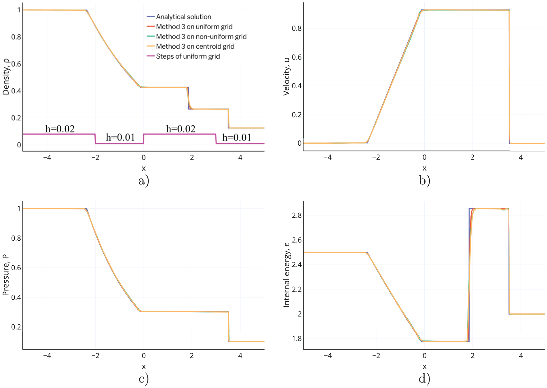
Figure 6: The distributions of (a) density, (b) velocity, (c) pressure, and (d) internal energy over space obtained by solving the Sod’s problem by Method 3 on uniform (red line), non-uniform (green line) and centroid (yellow line) grids for time
Fig. 7 shows a highly zoomed-in scale of the density profile after passing the transition (discontinuity) from coarse to fine grid in the direction of shock wave motion. On this scale, we can see the decrease of the density peak on the centroid grid.

Figure 7: The distribution of density over space on zoomed-in scale Fig. 6
The Sod’s problem is the most common problem in testing computational gas dynamics program packages because it contains zones of rarefaction wave, contact discontinuity, and shock wave. Comparing our calculations with [9], we note that both works have quite good results (without oscillations in the usual scale), although the calculations in [9] are performed on a finer grid (the space step length of which is equal to
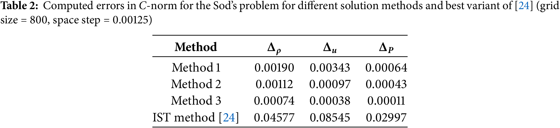
Table 2 shows that Method 2 and Method 3 have a fairly high calculation accuracy along with Method 1 and the IST method, with a smaller error by a factor of 2 or more. In addition, in our calculations there are fewer points in the shock wave zone than those of [24].
Table 3 shows the initial conditions of the Einfeldt’s problem [21]. The SI system is taken as the system of units in the calculations. The adiabatic index
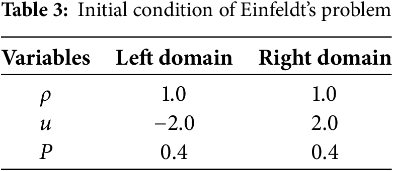
Since the efficiency of the methods developed in Section 3 has already been demonstrated in the Sod’s problem, the results of calculations using Methods 2 and 3 on uniform grid will be shown for the Einfeldt’s problem because of their higher efficiency compared to Method 1. All parameters
When calculating from the initial moment of time
4.2.1 Calculations of Einfeldt’s Problem
Using the analytical solution obtained by stitching the Riemann invariant with the constant flow zones [21], the right-hand position of the boundary of the stable “horizontal” zone is calculated by the formula
where
Fig. 8 presents the distributions of density, velocity, pressure, and internal energy from the initial moment
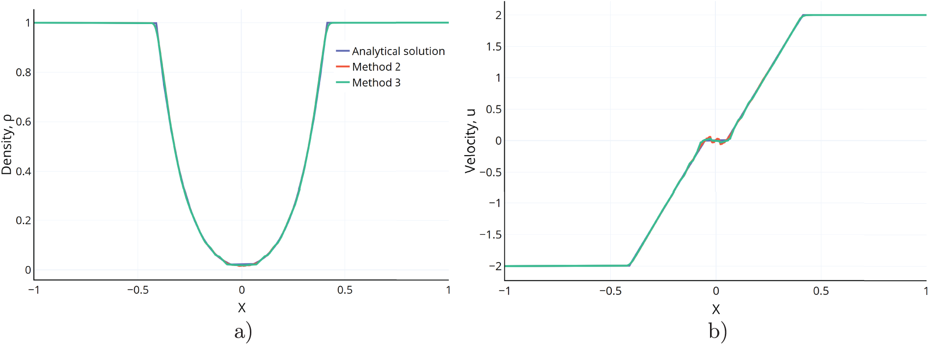

Figure 8: The distributions of (a) density, (b) velocity, (c) pressure and (d) internal energy over space obtained by solving the Einfeldt’s problem by Method 2 (red line) and Method 3 (green line) for time
Fig. 9 presents the distributions of density, velocity, pressure and internal energy from the initial moment

Figure 9: The distributions of (a) density, (b) velocity, (c) pressure and (d) internal energy over space obtained by solving the Einfeldt’s problem by Method 2 (red line) and Method 3 (green line) for time
In [19], the Einfeldt’s problem is also solved from the initial moment
The completely conservative difference schemes with adaptive artificial viscosity were considered, and the problem of modeling the gas dynamic processes described by equations in Euler variables was studied. The artificial viscosity method was shown as an effective way for improving the stability and suppressing the numerical oscillations. This work presented the effective methods for selecting adaptive artificial viscosity for completely conservative difference schemes. In particular, the improved method of explicit iterations with a predictor-correcting procedure was demonstrated. The developed methods were characterized by simplicity of realization. The calculations of classical Sod’s and Einfeldt’s problems were carried out to test the developed methods of artificial viscosity selection. Their results showed the efficiency and accuracy of the proposed methods. Comparing the results of this work with the analytical solutions and the calculation results of other authors was given. In addition, the method of velocity viscosity as an additive to pressure was proposed. The calculation results also showed the effectiveness of the velocity viscosity method for reducing the amplitude of the velocity and pressure profiles oscillations in the contact discontinuity zone. The grid embedding method was also developed, which improved the accuracy on a spatially non-uniform grid. The proposed mathematical method could be used to solve gas dynamics problems, including those with discontinuous data. The developed methods were not applicable to calculations with multi-temperature (two-temperature) approximations, as well as with non-isotropic force tensors acting in a continuous medium. In future works, it was planned to use the presented algorithms and methods in applied problems, as well as their generalization to the spatially multidimensional case.
Acknowledgement: The work of Marina Ladonkina, Viktoriia Podryga, Yury Poveshchenko was supported by KIAM RAS. The work of Haochen Zhang was supported by MIPT NRU.
Funding Statement: The work was carried out within the framework of the state assignment of KIAM RAS (No. 125020701776-0).
Author Contributions: The authors confirm contribution to the paper as follows: formal analysis and supervision: Marina Ladonkina; project administration and writing—review and editing: Viktoriia Podryga; conceptualization and methodology: Yury Poveshchenko; investigation, software, validation and writing—original draft preparation: Haochen Zhang. All authors reviewed the results and approved the final version of the manuscript.
Availability of Data and Materials: The data that support the findings of this study are available from the Corresponding Author, Viktoriia Podryga, upon reasonable request.
Ethics Approval: Not applicable.
Conflicts of Interest: The authors declare no conflicts of interest to report regarding the present study.
References
1. Popov YuP, Samarskii AA. Completely conservative difference schemes for the equations of gas dynamics in Euler’s variables. USSR Comput Math Math Phys. 1970;10(3):265–73. doi:10.1016/0041-5553(70)90133-3. [Google Scholar] [CrossRef]
2. Popov YuP, Samarskii AA. Completely conservative difference schemes. USSR Comput Math Math Phys. 1969;9(4):296–305. doi:10.1016/0041-5553(69)90049-4. [Google Scholar] [CrossRef]
3. Kuzmin AV, Makarov VL. An algorithm for constructing completely conservative difference schemes. USSR Comput Math Math Phys. 1982;22(1):128–38. doi:10.1016/0041-5553(82)90170-7. [Google Scholar] [CrossRef]
4. Kuzmin AV, Makarov VL. On one completely conservative difference scheme for the equation of gas dynamics in Euler variables. Comput Math Math Phys. 1980;20(1):171–81. doi:10.1016/0041-5553(80)90072-5. [Google Scholar] [CrossRef]
5. Popov IP, Fryazinov IV. Adaptive artificial viscosity method numerical solution of equations of gas dynamics. Moscow, Russia: Krasand; 2014. (In Russian). [Google Scholar]
6. Kurganov A, Liu Y. New adaptive artificial viscosity method for hyperbolic systems of conservation laws. J Comput Phys. 2012;231(24):8114–32. doi:10.1016/j.jcp.2012.07.040. [Google Scholar] [CrossRef]
7. Albright J, Shashkov M. Locally adaptive artificial viscosity strategies for Lagrangian hydrodynamics. Comput Fluids. 2020;205(3):104580. doi:10.1016/j.compfluid.2020.104580. [Google Scholar] [CrossRef]
8. Huang W, Ren Y, Tu G, Yuan X, Chen J. An adaptive artificial viscosity method for quintic spline reconstruction scheme. Comput Fluids. 2022;240(1):105435. doi:10.1016/j.compfluid.2022.105435. [Google Scholar] [CrossRef]
9. Wu Z, Ren Y. A shock capturing artificial viscosity scheme in consistent with the compact high-order finite volume methods. J Comput Phys. 2024;516(8):113291. doi:10.1016/j.jcp.2024.113291. [Google Scholar] [CrossRef]
10. Popov IV, Gasilov VA, Krukovskiy AYu, Boldarev AS. Difference scheme with adaptive artificial viscosity for gas-dynamic computations on nonuniform meshes. Math Models Comput Simul. 2024;16(Suppl 2):S263–71. doi:10.1134/S2070048224700960. [Google Scholar] [CrossRef]
11. Ogban PU, Naterer GF. Entropy-based artificial dissipation as a corrective mechanism for numerical stability in convective heat transfer. Numer Heat Transf B-Fundam. 2023;84(1):1–23. doi:10.1080/10407790.2023.2174625. [Google Scholar] [CrossRef]
12. Guermond JL, Nazarov M, Popov B, Tomas I. Second-order invariant domain preserving approximation of the Euler equations using convex limiting. SIAM J Sci Comput. 2018;40(5):A3211–39. doi:10.1137/17M1149961. [Google Scholar] [CrossRef]
13. Hennemann S, Rueda-Ramírez AM, Hindenlang FJ, Gassner GJ. A provably entropy stable subcell shock capturing approach for high order split form DG for the compressible Euler equations. J Comput Phys. 2021;426:109935. doi:10.1016/j.jcp.2020.109935. [Google Scholar] [CrossRef]
14. Zhang T, Zhan C, Cai B, Lin C, Guo X. An improved meshless artificial viscosity technology combined with local radial point interpolation method for 2D shallow water equations. Eng Anal Bound Elem. 2021;133(6):303–18. doi:10.1016/j.enganabound.2021.09.002. [Google Scholar] [CrossRef]
15. Yue M, Wang X, Liu Z, Cao W-D, Wang Y, Hu J, et al. Application of adaptive artificial viscosity method to reduce grid orientation effect in numerical simulations for steam thermal recovery. Arab J Sci Eng. 2025;50(13):10359–84. doi:10.1007/s13369-024-09865-y. [Google Scholar] [CrossRef]
16. Wang X, Yue M, Liu Z, Cao W, Wang Y, Hu J, et al. Numerical strategy on the grid orientation effect in the simulation for two-phase flow in porous media by using the adaptive artificial viscosity method. Int J Numer Anal Methods Geomech. 2025;49(2):541–54. doi:10.1002/nag.3886. [Google Scholar] [CrossRef]
17. Clinco N, Girfoglio M, Quaini A, Rozza G. Filter stabilization for the mildly compressible Euler equations with application to atmosphere dynamics simulations. Comput Fluids. 2023;266(2):106057. doi:10.1016/j.compfluid.2023.106057. [Google Scholar] [CrossRef]
18. Margolin LG, Lloyd-Ronning NM. Artificial viscosity-then and now. Meccanica. 2023;58(6):1039–52. doi:10.1007/s11012-022-01541-5. [Google Scholar] [CrossRef]
19. Rahimly OR, Poveshchenko YuA, Popov SB. Two-layer 1D completely conservative difference schemes of gas dynamics with adaptive regularization. Math Models Comput Simul. 2022;14(5):771–82. doi:10.1134/S2070048222050118. [Google Scholar] [CrossRef]
20. Sod GA. A survey of several finite difference methods for systems of nonlinear hyperbolic conservation laws. J Comput Phys. 1978;27(1):1–31. doi:10.1016/0021-9991(78)90023-2. [Google Scholar] [CrossRef]
21. Einfeldt B, Munz CD, Roe PL, Sjögreen B. On Godunov-type methods near low densities. J Comput Phys. 1991;92(2):273–95. doi:10.1016/0021-9991(91)90211-3. [Google Scholar] [CrossRef]
22. Bourgeois R, Tremblin P, Kokh S, Padioleau T. Recasting an operator splitting solver into a standard finite volume flux-based algorithm. The case of a Lagrange-projection-type method for gas dynamics. J Comput Phys. 2024;496(2):112594. doi:10.1016/j.jcp.2023.112594. [Google Scholar] [CrossRef]
23. Laibe G, Price DJ. Dusty gas with smoothed particle hydrodynamics-I. Algorithm and test suite. Mon Not R Astron Soc. 2012;420(3):2345–64. doi:10.1111/j.1365-2966.2011.20202.x. [Google Scholar] [CrossRef]
24. Nguyen V, Phan T, Park W. Numerical modeling of multiphase compressible flows with the presence of shock waves using an interface-sharpening five-equation model. Int J Multiphase Flow. 2021;135:103542. doi:10.1016/j.ijmultiphaseflow.2020.103542. [Google Scholar] [CrossRef]
25. Ladonkina ME, Poveschenko YuA, Rahimly OR, Zhang H. Theoretical study of stability of nodal completely conservative difference schemes with viscous filling for gas dynamics equations in Euler variables. Zhurnal SVMO. 2022;24(3):317–30. doi:10.15507/2079-6900.24.202203.317-330. [Google Scholar] [CrossRef]
Cite This Article
 Copyright © 2025 The Author(s). Published by Tech Science Press.
This work is licensed under a Creative Commons Attribution 4.0 International License , which permits unrestricted use, distribution, and reproduction in any medium, provided the original work is properly cited.
 Downloads
 Citation Tools