
 Submit a Paper
 Propose a Special lssue
 Open Access
ARTICLE

A Novel Multi-Step Numerical Framework for Ice Accretion Prediction Based on Unsteady Water Film Dynamics
1 School of Aviation Maintenance Engineering, Chengdu Aeronautic Polytechnic University, Chengdu, 610100, China
2 College of Aerospace Engineering, Nanjing University of Aeronautics and Astronautics, Nanjing, 210001, China
* Corresponding Author: Ke Shen. Email:
Frontiers in Heat and Mass Transfer 2025, 23(6), 1957-1980. https://doi.org/10.32604/fhmt.2025.070396
Received 15 July 2025; Accepted 17 October 2025; Issue published 31 December 2025
 View Full Text
 Download PDF
Abstract
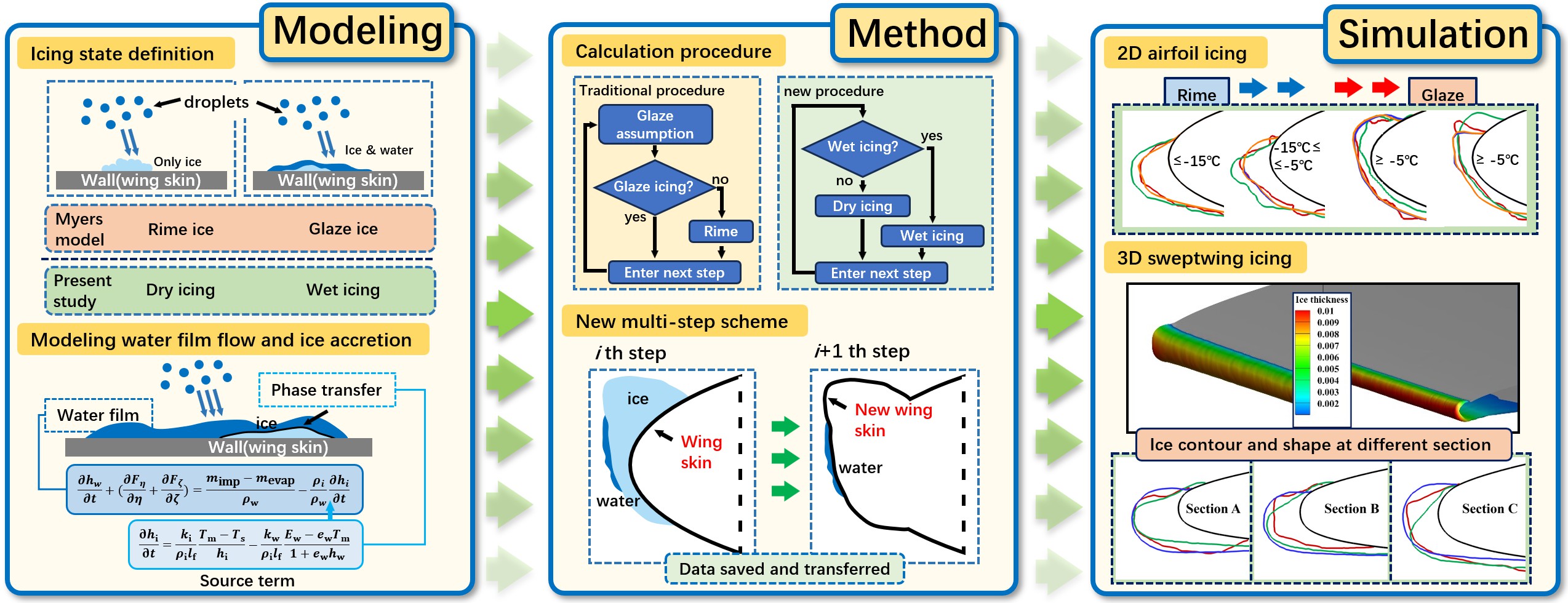
Ice accretion on aircraft poses a critical threat to flight safety by significantly altering aerodynamic performance. This study presents a novel numerical framework for ice accretion prediction, developed by extending the Myers model and incorporating an advanced multi-step approach. The proposed framework integrates ice layer growth into the modeling of unsteady water film dynamics and introduces a revised criterion for determining the icing condition. A multi-step scheme, accounting for the continuous variation of physical parameters, is implemented to enhance computational accuracy. The framework is validated through simulations on both 2D and 3D configurations. For the NACA0012 airfoil, the model demonstrates strong adaptability to both rime and glaze ice scenarios, with simulated ice shapes and thicknesses showing close agreement with experimental data, especially under low-temperature rime ice scenarios. In glaze ice cases, the framework effectively captures the leading-edge ice thickness and horn formation, albeit with minor positional deviations. For the GLC-305 swept wing, the approach accurately reproduces the primary ice shape features and overall thickness distribution. However, discrepancies in icing extent and thickness persist under rime scenarios due to the limitations of the single-step strategy. In glaze ice scenarios, the model captures the general trend of ice horn development, though positional and thickness deviations remain. Overall, the developed framework improves the precision of ice accretion simulations and offers a promising tool for advancing aircraft safety. Future research will aim to refine the multi-step framework to further improve its robustness and accuracy in complex, 3D icing environments.Graphic Abstract
Keywords
Clouds consist of water droplets, with many containing supercooled liquid water droplets that exist below the freezing point. When an aircraft encounters such super-cooled cloud layers during flight, ice can accumulate on the aerodynamic surfaces, thereby altering the aircraft aerodynamics and impacting its performance and stability, which may ultimately jeopardize flight safety [1]. Modern aircraft are typically equipped with anti-icing and de-icing systems, and the impacts of ice accretion are taken into account during the aerodynamic design phases. Consequently, the development of accurate and effective ice accretion prediction approaches is crucial for ensuring flight safety. For the aircraft icing issues, the types of ice can generally be categorized into three types [2]:
(1) Rime ice typically forms in low temperature environments, generally below −15°C, as a result of the freezing of water droplets. This type of ice usually exhibits a more regular and rounded shape, characterized by a porous internal structure and weak surface adhesion.
(2) Glaze ice forms in environmental conditions ranging from −10°C to 0°C. In contrast to the rapid formation of rime ice, the development of glaze ice occurs gradually, transitioning from a liquid water film to a solid state with a compact internal structure. Typically, glaze ice exhibits different characteristics associated with ice horns.
(3) Mixed ice, which occupies an intermediate position, exhibits characteristics of both rime ice and glaze ice. In its initial stage, the inner layer typically shows features associated with rime ice, while the outer layer in the later stage demonstrates characteristics of glaze ice [3].
While the above classification is commonly used, the present study will employ the terminology of “dry” and “wet” icing conditions in subsequent sections to better align with the physical processes described in the mathematical model.
Research on aircraft icing issues is typically conducted through two primary methodologies: experimental studies and numerical analyses [4]. Given considerations such as time efficiency, economic costs, and accuracy, numerical studies have emerged as the predominant approach for investigating ice accretion phenomena at present.
The fundamental aspect in numerical studies is mathematical modeling. Messinger [5] introduced the concept of a freezing coefficient, based on the classical Stefan problem. They made assumptions regarding the distribution of run-back water across the surface where ice forms, leading to the proposal of the classic Messinger model.
Building upon the Messinger model and its extended variants (e.g., Shallow Water Icing Model (SWIM) [6]), Myers and Hammond [7] introduced a novel model that addresses the dynamics of run-back water flow and the heat transfer through the ice layer on 3D surfaces. By incorporating the unsteady movement of run-back water and demonstrating adaptability to 3D scenarios, the Myers model has emerged as a leading focus in contemporary research.
Recent numerical studies addressing aircraft icing issues can be classified into two primary categories. Firstly, numerous studies focused on the factors that impact the ice formation process, including surface roughness and the impact of supercooled large droplets; Secondly, there is a significant focus on enhancing existing thermodynamic models of ice accretion, which includes considerations of heat conduction within the ice layer and the skin panel.
Focusing on the heat transfer processes that impact icing, Han and Palacios [8] developed a coupled model that incorporates both heat transfer and the evolution of surface roughness, subsequently integrating this model into the LEWICE-2D software. The conventional approach for calculating the convective heat transfer coefficient is the boundary layer integral method. Radenac et al. [9] utilized a finite volume boundary layer integration technique to enhance the accuracy of the convective heat transfer coefficient calculations within icing models, based on the assumption of smooth wall conditions. McClain et al. [10] formulated a model for the evolution of roughness in icing scenarios.
This paper focuses on the ice accretion model itself, highlighting significant developments from numerous related studies in recent years. Gori et al. [11] integrated the exact solution of the unsteady Stefan problem into the Myers model to determine the internal temperature distribution within the ice layer under glaze ice conditions, thereby aiming to enhance the accuracy of ice shape prediction. The effectiveness of this approach in improving precision was subsequently validated. Cao et al. [12] enhanced the Messinger model by incorporating the direction of airflow as a criterion for the flow direction of run-back water. Additionally, they proposed two multi-step schemes and conducted an analysis of their respective advantages and disadvantages. Lavoie et al. [13] performed a comprehensive review and comparative study of the Messinger model and its improved derivatives, as well as the SWIM, with a focus on assessing the simulation accuracy in replicating the behavior of run-back water. Liu et al. [14] utilizing the Phase-Field methodology and the Messinger model, introduced the Variational Spacing Grid (VSG) approach for solving one-dimension unsteady heat conduction based on the numerical solution of the non-steady-state Stefan problem. They modified the linear temperature distribution assumption within the Myers model, thereby enhancing its accuracy. Dai et al. [15] developed a novel ice accretion model, which has been validated under typical scenarios of rime ice and glaze ice. Li et al. [16] employed the Messinger model to determine the wall temperature during the ice accretion process, using the resulting temperature as the input parameters for the Myers model, thereby addressing the initial value problem of the bottom temperature of the ice layer within the Myers model. Nogi and Imamura [17] developed a new icing model based on the rigid sphere model, wherein ice particles are represented as rigid spheres, and the ice shape is depicted as a collection of these spheres. In both 2D and 3D scenarios, the simulated ice shapes qualitatively align with experimental results. Aguilar et al. [18] employed the self-developed two-dimensional software ICAT and based on experimental ice crystal icing data of the NACA0012 airfoil, so as to revise the ice crystal adhesion and erosion models, indicating that the effects of the water film and ice crystal particle morphology require further consideration under high total water content scenarios. Donizetti et al. [19] employed the PoliMIce platform and incorporating a level-set-based mesh reconstruction method, and performed the ice accretion simulation on a NACA0012 wing; the work demonstrated the critical role of multi-step computation in accurately capturing complex ice characteristics. Liu et al. [20] coupled a Messinger model incorporating non-spherical ice crystal drag, adhesion, and icing thermodynamics to conduct numerical simulations on a multi-element airfoil under mixed-phase icing scenarios. The results indicated that the ice crystal adhesion mass flux is significantly high, with adhesion occurring even in the runback region.
Currently, numerical research on aircraft icing has attained a relatively advanced stage, with several commercial software programs and platforms available. Notable examples include LEWICE developed by National Aeronautics and Space Administration (NASA) in the United States [21], FENSAP-ICE produced by Bombardier Transportation Institute (BTI) in Canada [22], and ONERA from the French Aerospace Research Center [23].
In a comprehensive analysis, the majority of contemporary numerical simulation studies concerning aircraft icing focus on enhancements to the Messinger and Myers models. However, both models exhibit certain limitations. The Messinger model is fundamentally a quasi-steady-state model, which fails to accurately represent the actual physical processes involved in the formation of water films and their gradual freezing during downstream flow. Furthermore, the Messinger model presents challenges in its adaptation to the multi-step schemes that are commonly employed in icing simulations. Additionally, due to the assumptions regarding the distribution of run-back water, the application of this model to 3D icing calculations, such as those involving swept wings, is also problematic.
The Myers model [24] enhances the Messinger model by integrating the unsteady water film dynamics equation derived from the Navier-Stokes equations and differentiating among various icing scenarios. This advancement allows for a more precise representation of the underlying physical processes in comparison to the Messinger model. However, the calculation procedure of the Myers model necessitates empirical assumptions regarding the initial water film and ice thickness. These assumptions may diverge from the actual physical processes, potentially introducing errors. Consequently, there exists an opportunity for further refinement in this aspect.
To achieve accurate icing simulation with broad applicability, this paper presents an enhanced calculation procedure based on the Myers model. This approach conceptualizes the phase transition of icing as a different phenomenon associated with the dynamics of a thin water film impacted by airflow shear stress, pressure gradients, and surface tension, rather than focusing on the dynamics of the water film during the icing process. Consequently, a novel numerical model for ice accretion and water film dynamics, along with the corresponding calculation procedure, has been developed.
2 Modeling of Water Film and Ice Layer
The physical process of ice accretion involves complex interactions between multiphase flow, heat transfer and phase change. A general framework for modeling this phenomenon can be derived from the fundamental conservation laws of mass, momentum, and energy. This section establishes such a general framework, which describes the formation and flow of water dynamics (a simplification of the Navier-Stokes equation based on the lubrication theory) and the subsequent growth of an ice layer (an unsteady Stefan problem) on a curved surface. The equations are presented in their most comprehensive form, from which established models, such as those by Messinger and Myers, can be derived as special cases under specific simplifying assumptions. The novel contributions of this study-namely, a revised icing condition criterion and an improved multi-step scheme are then introduced within this unified framework.
2.1 Icing Condition Definition
As Myers and Charpin [24] had presented, the process of ice layer formation is categorized into two types: “rime ice” and “glaze ice”. The direct freezing of supercooled water droplets upon impact corresponds to rime ice, while glaze ice is formed through the freezing of a flowing water film.
While the traditional classification in the introduction section is widely used for describing ice morphology, this study adopts the concepts of “dry icing” and “wet icing” to provide a more physically-based classification that better aligns with the underlying thermodynamic processes. Specifically, “dry icing” corresponds to conditions where all impinging water freezes immediately (typically associated with rime ice), while “wet icing” describes conditions where liquid water persists and flows before freezing (typically associated with glaze ice). This terminology shift aims to reduce semantic ambiguity in the mathematical modeling of the icing process.
To further clarify, as shown in Fig. 1, the condition in which all water droplets freeze instantaneously upon surface impact is defined as “dry icing”. Conversely, “wet icing” refers to the condition in which only partial freezing occurs upon impact, resulting in the formation of a surface water film due to the convergence of unfrozen droplets.
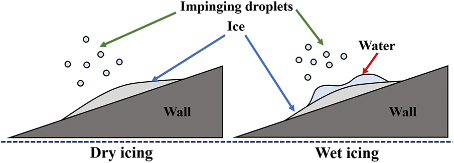
Figure 1: Schematic of dry/wet icing conditions
The dry icing condition can be understood as a direct phase transition from liquid water droplets to an ice layer, occurring in the absence of a liquid water film. Consequently, the calculation of rime ice is relatively simple, and most icing models are able to produce satisfactory results. In contrast, the dynamics of the water film have a significant impact on the wet icing condition, which is the primary focus of this study. Therefore, it is imperative to first present the governing equations that describe the flow of a water film over arbitrary 3D surfaces.
2.2 Modeling of Water Film Dynamics
At higher freezing temperatures, the impacting water droplets undergo complete solidification only during the initial transient period. Subsequently, partial solidification occurs, resulting in the formation of a water film or run-back water that traverses the surface. The actual flow dynamics are highly complex and impacted by a multitude of factors. For aircraft icing, however, the thickness of the film is typically on the order of micrometers, and the temperature is approximately 0°C (273.15 K). These characteristics allow for the adoption of certain assumptions to facilitate a simplified analysis [24,25].
(1) The dynamic viscosity, specific heat capacity, and surface tension of water are regarded as constants, with values typically referenced at 0°C (273.15 K).
(2) The thickness of the water film is negligible in comparison to the extent of its spread, denoted as l. Therefore, the flow velocity of the water film in the direction normal to the wall surface is disregarded. Additionally, the dimensionless parameter ε2Re (ε = hw/l) is also regarded as very small.
(3) As mentioned in (2), although the hydrophilic/hydrophobic properties of the solid surface affect the contact angle between the water film and the wall, and thereby influencing the morphology of the film front, the morphological characteristics of the water film are still physically minute at this scale. Therefore, morphological changes at the moving leading edge of the water film are neglected.
(4) In the calculations, it is assumed that the surface is smooth and clean, so that the water film flows over which is sufficiently smooth and not be affected by the roughness, thereby neglecting the impact of surface roughness on the flow of the water film.
To characterize the motion of a thin water film on a curved surface, a body-fitted coordinate system can be established within a 3D framework (Fig. 2). This Body-fitted coordinate system is represented by the coordinates (ξ, η, ζ), where ξ and η tangential to the surface, while ζ serves as the outward normal vector at that point, remaining perpendicular to both ξ and η. The wing surface corresponds to the condition where ζ = 0. Any position on this surface can be represented by the position vector R(η, ξ).
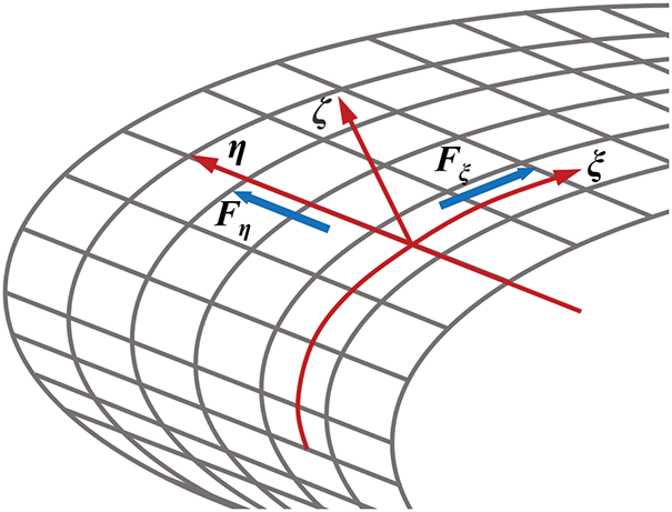
Figure 2: Body-fitted coordinate system for 3D curved surface
Based on the previously stated assumptions, the first and second fundamental quantities, represented by (e1, e2, e3) of the differential geometry are employed to derive the Navier-Stokes equations within a body-fitted coordinate system, yielding the following expressions [24]:
where Pw and ρw represent the pressure and density of the water film, respectively; Vξ, Vη, and Vζ represent the contravariant velocities in the ξ, η, and ζ directions, respectively; fξ and fη represent the components of the body force in the direction of ξ and η, respectively (on the surface of a non-rotating body, there are no inertial forces, so only the gravity needs to be considered), and O represents the higher-order infinitesimal operator. And:
where μw represents the dynamic viscosity of the water film.
The first fundamental quantities (coefficients) of the surface mentioned before are denoted by e1, e2, and e3, respectively:
At the wing surface where ζ = 0, the no-slip boundary condition yields:
Considering the scenario where the water film at the bottom freezes to form ice, the velocity component in the ζ direction is non-zero. Consequently, the relationship between the velocity component Vζ and the rate of ice layer growth is as follows:
For a scenario in which the water film at the base freezes to form ice, the velocity component in the ζ direction is non-zero. Therefore, the relationship between the velocity component Vζ and the growth rate of the ice layer can be expressed as follows:
where Aξ and Aη represent the components of the aerodynamic shear stress in the ξ and η directions, respectively. The velocity component Vζ in the ζ direction can be determined as follows:
The volumetric flow rates along unit depth in the ξ and η directions (Fξ and Fη) are obtained by integrating the water film flow velocity over the thickness ζ in both the ξ and η directions:
The factors that impact the flow of the water film on the wing surface can be simplified to three primary components: aerodynamic shear stress, pressure gradient, and body forces.
By incorporating the mass of impinging water droplets mimp, the mass inflow from upstream run-back water and the mass of evaporated liquid water mevap as source terms, the mass balance equation for the water film flow can be further developed. This equation utilizes the water film thickness hw as the fundamental variable:
Eq. (10) comprises a time-dependent term on the left-hand side, referred to as the unsteady term, along with the convective term and the source term on the right-hand side. This structure is similar to the classical form of the single wave equation commonly encountered in Computational Fluid Dynamics (CFD).
The system of equations is presented in 3D form. However, for 2D scenarios, the set of equations can be simplified through dimensional reduction.
In scenarios where the angle of attack of the incoming flow is zero relative to the far field, it can be inferred that the velocity of any point on the object is equivalent to the far-field flow. This condition is exemplified by fixed-wing aircraft. The computational methodology employed for mass incoming from droplet impingement mimp is outlined as follows:
where LWC (Liquid Water Content) represents the liquid water content; V0 represents the far-field incoming flow velocity; and β represents the local water collection efficiency.
The comprehensive formulation of the governing equations for water film dynamics, derived from a curvilinear coordinate system, is complex and entails geometric transformations rooted in differential geometry, which can substantially elevate computational demands. Therefore, Myers and Charpin [26] suggested that, for the purposes of practical calculations, it is acceptable to approximate the surface as a plane to facilitate simplification. This approach was similarly adopted by the software ICECREMO. The simplified formulation is presented as follows:
The mass balance equation governing the water film dynamics during the freezing process is formulated as follows:
where ρi and ρw represent the density of ice and water, respectively; and mevap represents the mass loss rate due to evaporation. Eq. (13) represents the mass balance equation for the flow of the water film. The accumulation of ice indicates a decrease in the thickness of the water film, which is incorporated into the equation as a source term.
The set of equations presented above constitutes a general formulation for unsteady water film dynamics on a 3D surface. Simplifications of the general framework lead to established models. For instance, the Messinger model [5] can be viewed as a case that neglects the unsteady and convective terms in the water film flow, assuming a quasi-steady, uniform film distribution. While the Myers model [24], in turn, is a significant advancement that retains the full unsteady and convective physics of the water film, as represented in this section, but employs a different criterion for icing condition transition.
In both dry icing and wet icing scenarios, phase transitions and heat transfer processes are integral components, which will be elaborated upon in the subsequent chapter. Generally, the thickness of the ice layer is significantly smaller than the characteristic length of the wing, often by an order of magnitude, and the rate of increase in thickness is considerably less than both the velocity of the water film flow and the freestream velocity. In this study, the following assumptions are made when analyzing the growth rate of ice layers on the wing surface:
(1) The analysis focuses only on the conduction of heat within the ice layer and the water layer perpendicular to the wing surface, treating the heat conduction process as a quasi-static phenomenon.
(2) The contact thermal resistance at the interface is disregarded, and it is assumed that the temperature at the base of the ice layer is equivalent to the wing surface.
(3) For various icing conditions, the density of ice is assumed to be constant.
(4) The thickness of the ice layer is assumed to increase monotonically, without any decrease. Therefore, the phenomena of ice layer melting and shedding are not considered.
Fig. 3 illustrates the schematic representation of control volumes and surface heat fluxes for both dry icing and wet icing conditions. Ts represents the wall temperature, which corresponds to the temperature at the base of the ice layer. Tf represents the surface temperature of the outermost medium within the control volume. In a control volume devoid of ice or water, Tf represents the equivalent to Ts. Ti and Tw represent the temperatures within the ice layer and the water layer, respectively.
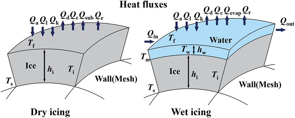
Figure 3: Heat fluxes distributions for dry and wet icing condition within a control volume, where Qk represents the kinetic energy of water droplet impact; Qa represents the aerodynamic heating heat flux; Ql represents the latent heat of freezing; Qd represents the sensible heat of water droplets; Qc represents the convective heat flux from the air; Qevap represents the evaporative heat flux; Qsub represents the sublimation heat flux; and Qr represents the radiative heat flux
In the dry icing condition, it is assumed that no liquid water exists within the control volume, and only sublimation is taken into account. Conversely, in the wet icing condition, the presence of a water film as the outermost layer of the control volume necessitates the consideration of evaporation exclusively. The mass balance equation for a control volume in the dry icing condition is articulated as follows:
where min represents the mass of upstream run-back water; and msub represents the mass loss rate of sublimation. On the surface of ice layer, the energy balance equation is expressed as follows:
where the intermediate variables Ed and ed, are introduced and reformulated the temperature distribution as follows:
Ed and ed are as follows:
here, Ta represents the static temperature of the airflow at that point, and Td represents the droplet temperature, which is generally the same as the airflow temperature.
qh denotes the convective heat transfer coefficient, which can be obtained from airflow field data. The other coefficients qflux, such as qs, qr, and qd, represent the ratios of the heat flux terms (i.e., Qs, Qr, and Qd) to the temperature difference between the air and the ice layer. These coefficients process no distinct physical essence but serve merely as intermediate variables.
The temperature distribution within the ice layer can be expressed as follows:
Under the wet icing condition, the heat balance equation at the surface of the control volume is expressed as follows:
Additionally, Ew and ew are introduced as follows:
where:
and qe represents the coefficient for the evaporation term. According to the classical Stefan problem, the rate of phase transition between ice and liquid water can be described by the heat conduction occurring within both the ice layer and the water layer.
where lf is the latent heat of ice formation, and in the Myers model, the icing condition is determined by the thickness of the ice layer, denoted as hi within the control volume. When hi increases to the critical thickness hi,crit, the condition transitions from dry to wet. By substituting Ti = Tm and ξ = hi into Eq. (20) the critical thickness hi,crit can be derived as follows:
When hi < hi,crit, the icing condition is dry and otherwise wet. In practical applications, four scenarios may arise, corresponding to the icing conditions in Table 1.
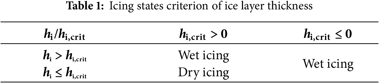
The variables such as the mass loss rate (mevap and msub) and the heat flux (Qflux) along with their corresponding computational methods are consistent in reference [24].
The energy balance and ice growth models described herein, coupled with the general water film equations from Section 2.2, form a complete thermodynamic framework. The novelty of the present approach lies in the use of the surface temperature Tf as the primary criterion for transitioning between dry and wet icing conditions. The change enhances the compatibility of the model with multi-step simulations, as Tf is a continuous variable that can be naturally inherited between steps, unlike the geometry-dependent ice thickness.
3.1 Overall Procedure of Ice Accretion Simulation
The foundational framework for icing numerical simulation was introduced by MacArthur [27] (Fig. 4). This framework can be categorized into four modules.
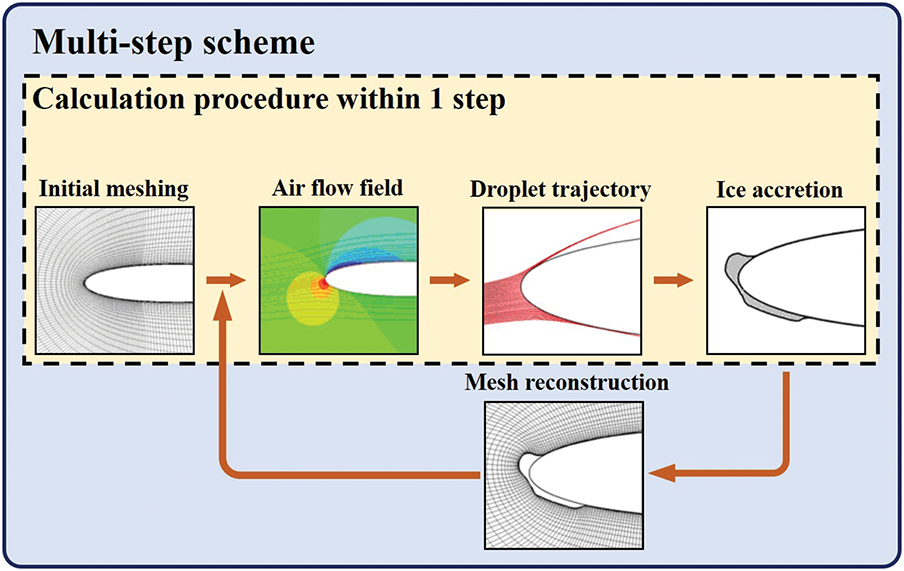
Figure 4: The simulation framework of ice accretion
To date, the framework has not experienced substantial modifications and remains extensively employed. Within this framework, the simulation commences with grid generation and CFD analysis of the flow, followed by the determination of water droplet trajectories and the accumulation of water on the icing surface, based on the airflow field data. Subsequently, an icing model is implemented to calculate the ice thickness at various locations. The grid of the icing surface is then adjusted in accordance with the computed ice thickness, resulting in the generation of the icing shape.
Currently, the majority of numerical studies pertaining to icing phenomena are conducted within this established framework, and the overall framework for icing simulation presented in this paper aligns closely with it. The multi-step approach disaggregates the ice accretion process, which was previously computed in a singular instance, into several discrete steps, thereby enhancing the accuracy of the simulations. Upon reaching the icing exposure duration designated for one step, a mesh reconstruction is executed in accordance with the configuration of the ice accretion. Utilizing the newly generated mesh, the processes of airflow field computation, water droplet impact characteristic assessment, and icing calculation are iteratively performed until the cumulative icing exposure time is achieved.
Aircraft icing represents a fundamentally unsteady phenomenon. Theoretically, incorporating a greater number of unsteady factors into the analysis will yield numerical results that more closely approximate the actual physical processes involved. Most numerical studies of ice accretion utilize a single-step scheme, wherein the ice layer is allowed to grow only once to achieve the final results. This approach calculates the amount of freezing and generates the ice shape based directly on parameters related to flow, heat transfer, and droplet impingement, all of which are determined under conditions of a clean airfoil.
The physical process of ice accretion involves the growth of an ice layer, which alters the aerodynamic shape of the surface. This change subsequently impacts the trajectory of water droplets and their collection characteristics on the surface, as well as the heat transfer properties of that surface. Therefore, from a methodological perspective, the single-step scheme is prone to substantial errors.
The multi-step scheme takes into account the impact of ice growth on the airflow field and the trajectory of water droplets, thereby providing a representation that more accurately reflects the actual physical processes involved. For the mathematical models of ice accretion, such as those proposed by Messinger or Myers, the computational results derived from the multi-step scheme generally demonstrate greater accuracy and reliability compared to those obtained through the single-step scheme.
In the computational framework of the multi-step scheme, updates to the mesh are integral to the process. Following each reconstruction of the mesh, both the normal vector of the surface grid, which determines the direction in which nodes will move, and the corresponding area will experience changes. For the Myers model, the thickness of the ice layer is defined in relation to the thickness of the ice layer along the ξ direction of the curvilinear coordinate system. When employing the multi-step scheme, it is essential to retain the thickness data at the conclusion of the previous step and to carry this data forward into the subsequent time step. Given that ξ varies with the mesh, if the ice thickness is utilized as a criterion for determining the icing conditions (either dry or wet), it becomes necessary to reconstruct the ice thickness in the ξ direction at the commencement of each time step. This process entails complex geometric calculations.
To improve the previously mentioned aspects and to better align the icing calculation with the multi-step scheme, this paper proposes a modification to the criterion for icing conditions. Specifically, the criterion is shifted from the critical thickness hi(crit) as defined in the Myers model to the surface temperature Tf. For any designated control volume or node, Tf is determined by the energy balance equation and exhibits continuous variation over time. If Tf falls below the triple point temperature of water Tm (273.15 K) at time of t, the icing condition is classified as dry icing. This classification assumes that all impinging water and run-back water entering the control volume during the subsequent time increment Δt will freeze completely, resulting in the absence of liquid water at t + Δt. Conversely, when the surface temperature reaches or exceeds Tm, the condition is classified as wet icing. In this scenario, only a portion of the impinging water and run-back water upstream freezes, while the remainder gradually flows downstream, propelled by airflow or surface tension, ultimately freezing at a later stage. Once the icing condition transitions from dry to wet, both the surface temperature of the ice layer and the bottom temperature of the water film will remain at Tm until the end of the process.
In the computational process described, the temporal variation of surface temperature Tf, is intricately linked to the equilibrium of various heat fluxes. For instance, under scenarios of glaze ice, the phenomenon of ice horn formation is frequently observed. This occurrence is attributed to the significant contribution of convective heat flux Qc, which cools the surrounding area, coupled with the presence of run-back water upstream that supplies sufficient liquid water for freezing. Airflow at temperatures below 0°C perpetually cools the region, while the latent heat released during the freezing of liquid water is rapidly dissipated, facilitating the development of ice horns. In the multi-step scheme employed in this study (Fig. 5), the ice shape generated in the preceding step is utilized as the “clean airfoil” for the subsequent iteration. During each step, the ice layer is incrementally added from the top of the ice shape calculated in the prior step. The surface temperature Tf at the conclusion of the previous step is utilized to initialize the wall temperature Ts for the next step, rather than consistently assigning the base temperature of the ice layer to T∞, which represents the far-field temperature and the predetermined icing temperature.
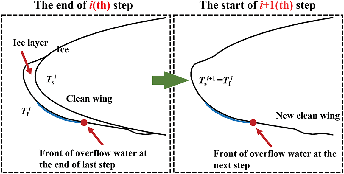
Figure 5: Approach of parameter transfer in the multi-step scheme
The aforementioned approaches guarantee the continuity of the key variable Tf, which is critical in determining the icing conditions, across consecutive steps.
Due to the minimal thickness of the water film and the neglect of internal heat storage within the film, the water film thickness hw (when present) in each element can inherit the results from the preceding step. With the introduction of the dynamic mesh method for reconstruction, the area of the mesh cells undergoes changes. If the hw were to be directly transferred, it would contravene the principle of mass conservation. Given that the density of the water film remains constant, what is actually transferred and inherited is the total volume of the water film in each element. Consequently, the relationship between the water film thickness across consecutive steps is outlined as follows:
In the Eq. (27),
3.3 Calculation Procedure of the Model
Fig. 6 illustrates the numerical calculation procedure for Myers model [24].
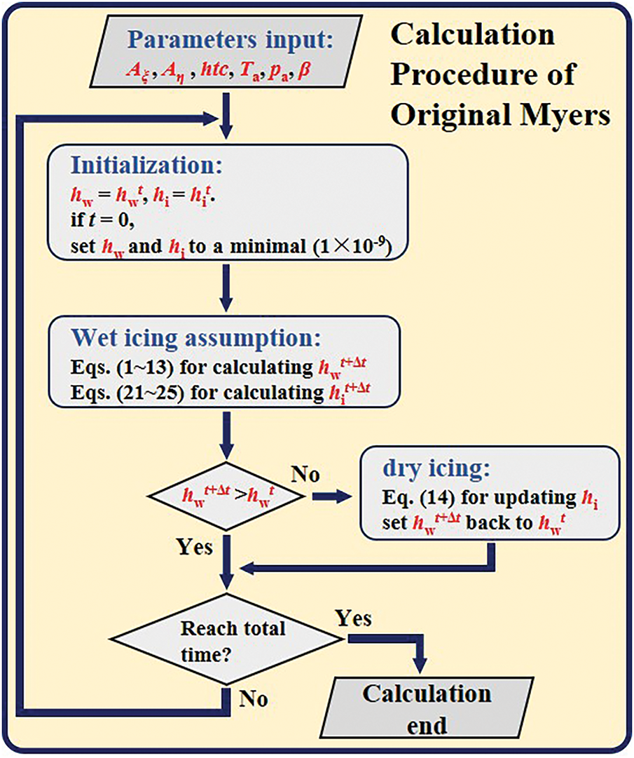
Figure 6: Calculation procedure of the original Myers model
Firstly, the ice thickness hi and water film thickness hw are assigned small empirical values, typically on the order of 1 × 10⁻⁶ m empirically, to initialize the calculation; Secondly,
For any control volume element, even when the condition of icing is classified as dry icing, the procedural mechanism allows for the presence of a minimal quantity of liquid water. This consideration is a mathematical abstraction and does not accurately reflect the underlying physical processes. Furthermore, the hypothesized water film plays a role in the resolution of the governing equations pertaining to water film flow, which introduces inaccuracies during the time marching process that compromise the mass conservation of the model. This paper presents a modified and novel calculation procedure designed to address this issue.
Fig. 7 depicts the modified numerical calculation procedure, which is predicated on the unsteady water film dynamics equations derived from the Myers model. The fundamental premise of this procedure is to conceptualize ice accretion as a different phenomenon for water film dynamics, in contrast to conventional phase transition models that treat water film flow as a component of the icing process. At each iterative time step, the governing equations pertaining to water film flow and ice accretion are resolved for all elements of the icing surface. Firstly, the icing condition (wet or dry) is determined based on the current temperature of Tf; Secondly, the rate of ice layer growth is computed utilizing various mass and energy balance equations: Eq. (5) is employed for dry icing conditions, while Eqs. (11)–(15) are utilized for wet icing conditions. For scenarios characterized by dry icing, Tf is updated at each step in accordance with Eqs. (6)–(10); Thirdly, the calculated ice layer growth rate is incorporated as a source term into Eqs. (1)–(3).
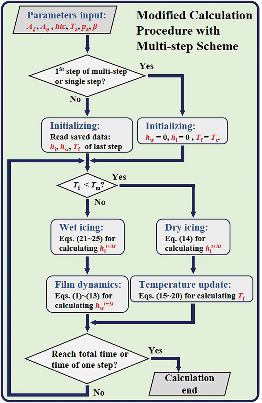
Figure 7: Modified calculation procedure of the icing model
The aforementioned procedure does not necessitate initial value assumptions, which are required in the original Myers calculation method, and it ensures the conservation of ice and water mass throughout the calculation domain during the time marching process. To solve (1)–(3), the finite volume method is employed for spatial discretization. The grid utilized is based on the wall grid used in previous CFD calculations, and a second-order upwind scheme is implemented to resolve the fluxes Fη and Fζ. For the time marching aspect, a third-order Runge-Kutta marching scheme is applied for explicit integration. The time step Δt is established at the global minimum, with Δt = 1 × 10⁻³ s, which generally satisfies the requirements for both calculation accuracy and robustness.
4.1 CFD Calculations of the NACA0012 Airfoil
The numerical simulation on a NACA0012 airfoil was conducted following the procedure outlined in Fig. 4. The airflow field was computed by a solver developed based on the open-source Free-CFD code, which solves the Reynolds-Averaged Navier-Stokes (RANS) equations. The classical Spalart-Allmaras model was selected as the turbulence model. Upon convergence of the airflow field computation, the resulting dat a were exported to the droplet trajectory calculation module.
The airflow field and the droplet field are computed in a one-way coupling manner. Given that the volume fraction of water droplets is extremely small, on the order of 10−6, the convective heat transfer coefficient and shear stress on the airfoil surface are extracted from the converged airflow solution, while the local water collection coefficient is obtained from the droplet field results. These parameters are then incorporated into the icing model developed in this study. Fig. 8 presents a comparison of the surface pressure coefficient and water collection coefficient for the NACA0012 airfoil under a specific scenario [28] (angle of attack AOA = 4°, freestream velocity V0 = 67.11 m·s−1, static temperature T0 = 244.80 K, static pressure p0 = 101,325 Pa).
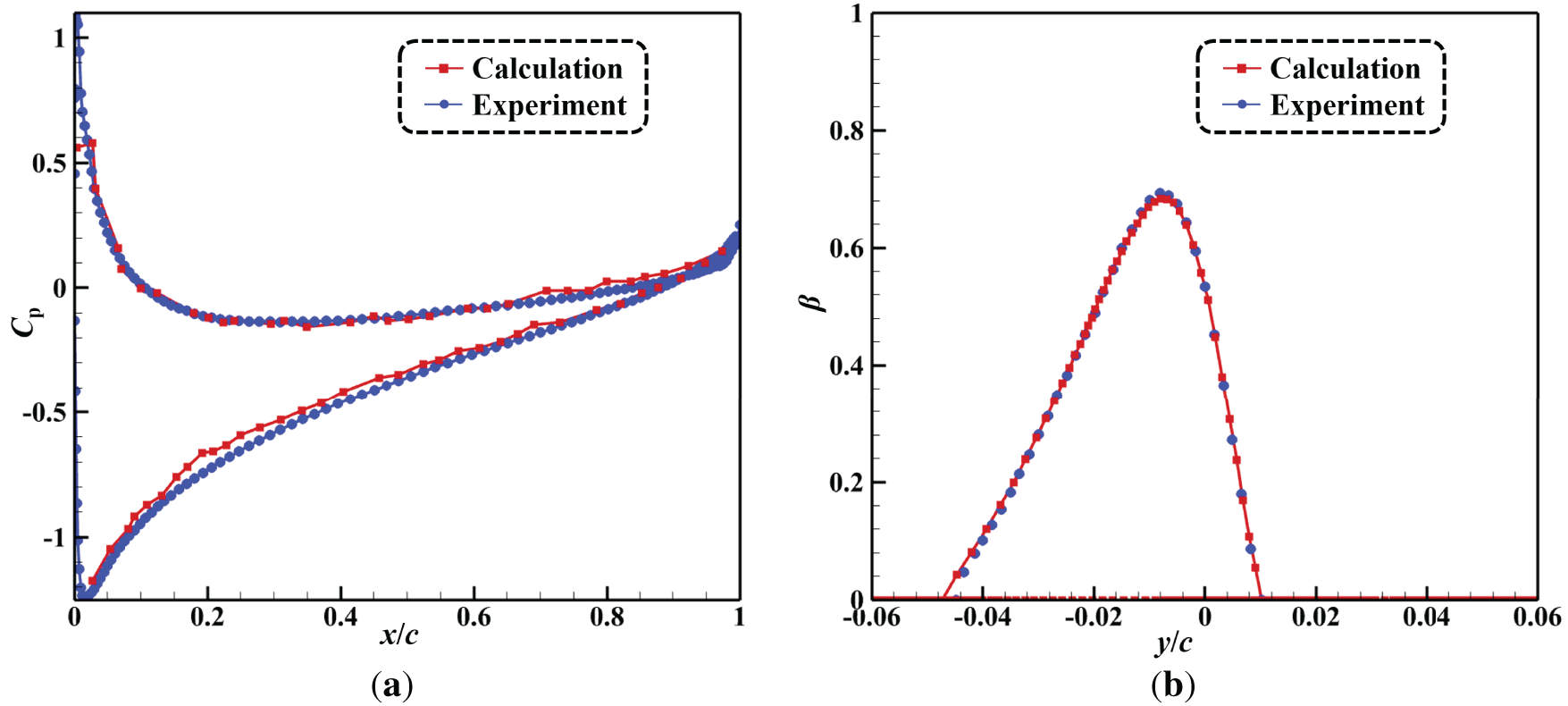
Figure 8: Comparison of surface pressure coefficient Cp for (a), and water collection β distribution for (b)
The icing model solves for the ice accretion growth over a small time increment: one step within a multi-step approach. After the specified time period elapses, the grid nodes are displaced using a dynamic mesh method based on ice thickness hi. The mesh regeneration approach employed in this study utilizes a dynamic mesh method based on the Delaunay graph and radial basis function (RBF) [29], which combines the capability of RBF-based mesh deformation to generate high-quality grids near moving boundaries with the computational efficiency of the Delaunay graph mapping method. The grid morphology at each step of the multi-step process (6 steps in this case) is shown in Fig. 9. Once the dynamic mesh module generates the updated grid, the entire process of airflow field computation, droplet trajectory calculation, and ice accretion simulation is repeated iteratively until the total icing exposure time is reached.
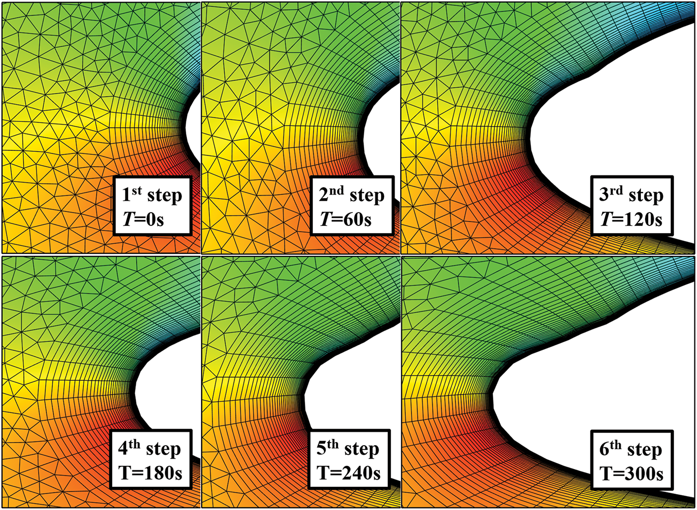
Figure 9: The dynamic mesh of Case. 1 in multi-step scheme
4.2 Ice Accretion Simulation on NACA0012 Airfoil
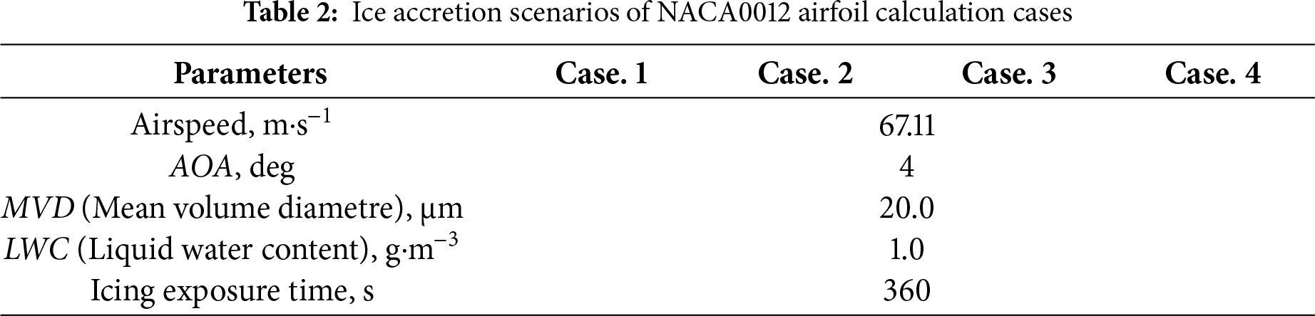
The validation study focused on the NACA0012 airfoil, which has a chord length of 0.5334 m. Simulations were conducted under three icing scenarios, characterized by increasing temperatures, and designated as Case. 1, Case. 2, Case. 3, and Case. 4, respectively.
The icing temperatures, also referred to as free-stream temperatures, for the cases under consideration are 244.8 K, 253.7 K, 267.6 K, and 268.4 K. To furnish a thorough reference, NASA experimental data and LEWICE computational results [30–32] have been included in the comparative analysis.
In addition to the icing temperatures, all other parameters are maintained consistently (Table 2). The calculations are conducted using a six step scheme, with updates to the grid, airflow field, and droplet impact characteristics occurring every 60 s.
The icing temperature serves as the sole variable differentiating Case. 1 from Case. 4, revealing a consistent pattern in the morphological changes of ice. In Case. 1, characterized by a lower ambient temperature, the resulting ice exhibits a smoother morphology typical of rime ice, as corroborated by experimental data, as shown in Fig. 10. Conversely, Case. 3 and Case. 4, which operate at a higher temperature, produces ice with pronounced horn features, a phenomenon that this study partially captures through calculations. Case. 2, which is situated at a medium temperature, shows a hybridization of characteristics from both rime and glaze ice; it demonstrates a trend towards ice horn development, albeit to a lesser extent than that observed in rime ice. Case. 1 represents a typical rime ice scenario. In Fig. 10a, the calculated results presented in this study demonstrate a closer alignment with the experimental data compared to the LEWICE model, particularly in terms of overall ice thickness. The accuracy of numerical simulations for rime ice scenarios is significantly impacted by the assessment of water droplet impingement characteristics. The enhancements made to the icing model in this study focus on the wet icing condition, taking into account the dynamics of the water film. Consequently, the improvement observed in the calculations for Case. 1 can be predominantly attributed to the implementation of the multi-step scheme.

Figure 10: Ice shape comparison on the NACA0012 airfoil for (a) Case 1, (b) Case 2, (c) Case 3, and (d) Case 4
While Case. 3 and Case. 4 typically represents a glaze ice scenario characterized by elevated temperatures, wherein the morphology of the ice is impacted by the wet icing condition. In both Fig. 10c,d, the results obtained from the LEWICE model exhibit substantial discrepancies in both the position and thickness of the ice ridge, as well as in the upper limit of the icing extent, when compared to the experimental data. In contrast, the results derived from the Myers model and this study demonstrate a high degree of similarity, providing a better fit to the experimental data than LEWICE. The overall ice shape and thickness align more closely with the experimental observations, and the horn feature is accurately represented. Close-up views in Fig. 10c,d reveal that, compared to the conventional Myers model, the presented model predicts slightly lower ice thickness at the stagnation area and slightly greater thickness near the ice horns. The difference is likely attributable to modifications in the computational method of the model, which had been introduced in Fig. 7. Elsewhere along the leading edge, the predicted ice thickness remains largely consistent between the two results. However, a minor deviation is noted in the upper limit of the icing extent.
The temperature of Case. 2 falls between those of Case. 1 and Case. 3, exhibiting characteristics of both rime and glaze ice. In contrast to the smooth texture of rime ice, Case. 2 shows a slight tendency towards horn growth, although this is not pronounced. In Fig. 10b, the ice morphology derived in this study closely resembles that reported by Myers. While both calculated results exhibit discrepancies in thickness when compared to the experimental data, they generally align with the results of LEWICE.
4.3 Ice Accretion Simulation on GLC-305 Swept Wing
In this section, the established numerical model and the calculation procedure are further validated using the 3D GLC-305 swept wing. The geometric model, along with its dimensions, is depicted in Fig. 11.
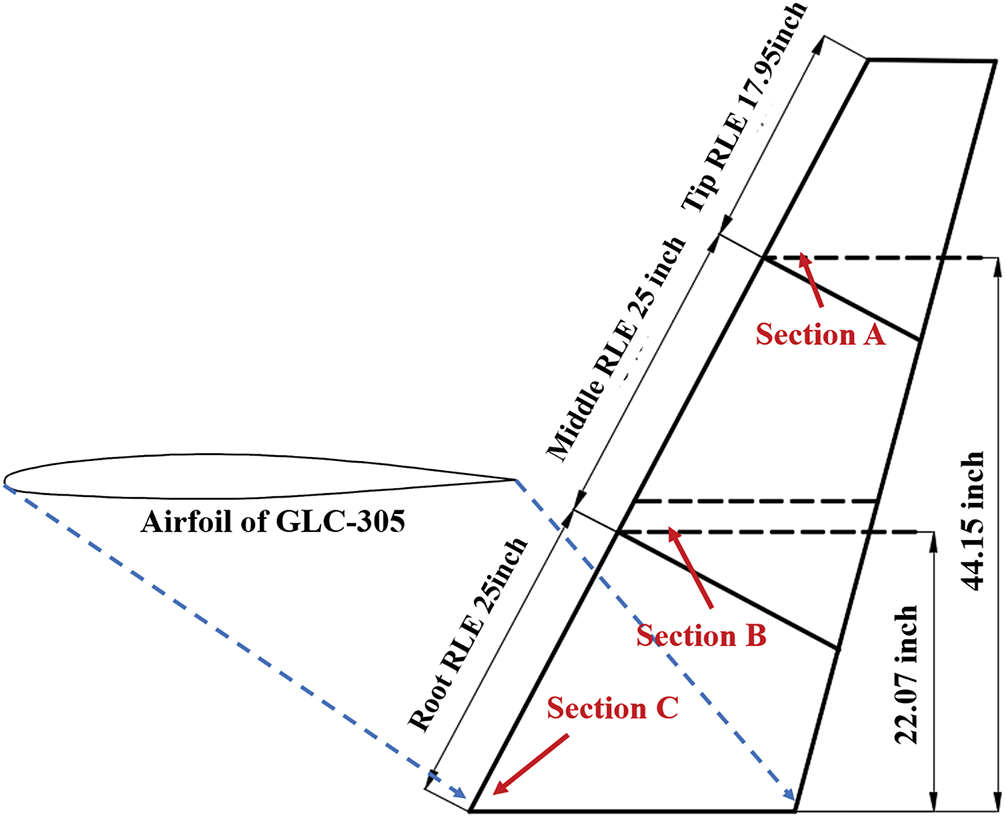
Figure 11: Geometry of GLC-305 wing and location of section A, B, and C
In 3D scenarios, the multi-step simulation imposes stringent requirements for mesh reconstruction due to the complex shapes of ice. However, the complexity of these ice shapes makes it challenging to ensure the quality of the mesh. Consequently, in the 3D ice accretion calculations presented in this section, only the single-step simulation is employed to assess the adaptability and accuracy of the model for 3D cases. The ice accretion scenarios are derived from Papadakis et al. [33], and the results are compared with both experimental data and LEWICE calculations.
For Case. 5 and Case. 6, the icing temperatures (far-field freestream temperatures) are 257.80 K and 263.0 K, respectively. And other parameters in relation to the calculation are in Table 3:
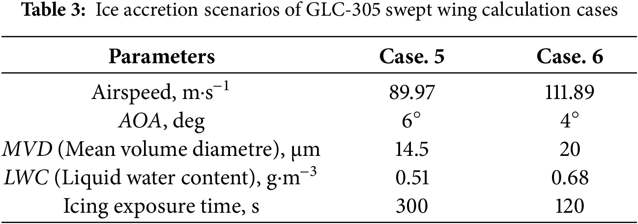
Fig. 12 shows the calculated contour of ice thickness at the front edge of the GLC-305 swept wing for Case. 5.
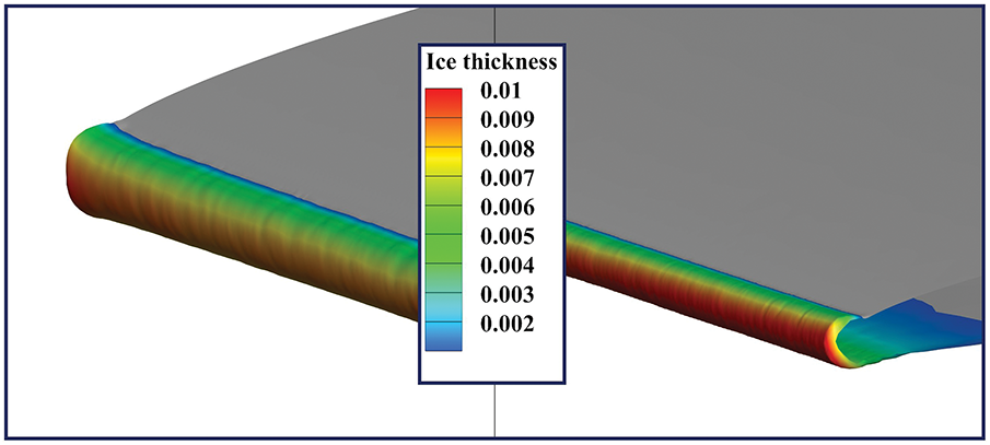
Figure 12: Ice layer contour of GLC-305 swept wing for Case 4
Figs. 13 and 14 depict the calculated ice formations for various sections of the wing in Case. 5 and 6. Case. 5 is characterized by low temperatures, which yield ice shapes that align with the characteristics of rime ice. In Fig. 13, the ice formations across all sections exhibit a relatively smooth surface, devoid of significant protrusions or indentations.

Figure 13: Comparison of ice shape on GLC-305 swept wing of Case. 5 for (a) Section A, (b) Section B and (c) Section C

Figure 14: Comparison of ice shape on GLC-305 swept wing of Case. 6 for (a) Section A, (b) Section B and (c) Section C
In section A of the wingtip, the computational results presented in this study demonstrate a favorable alignment with the experimental data, slightly surpassing the performance of LEWICE. The upper limit of the icing extent is relatively well matched. However, a significant discrepancy is observed in the lower ice limit. It is hypothesized that this discrepancy arises from the limitations of the single-step scheme, which fails to adequately capture the shielding area formed downstream as a result of ice accumulation on the leading edge. This inadequacy leads to an overestimation of water collection near the impingement limit, thereby contributing to a larger error in the ice limit. Furthermore, under the positive angle of attack condition in Case. 5, the deviation at the lower ice limit is more significant. In section B of the mid wing, the overall ice thickness derived from the computational results exceeds that observed in the experimental data. Similar to section A, there remains an issue with the deviation of the icing extent limit, attributable to the same factors. In section C at the root, a significant deviation in thickness is also evident between the computational results and the experimental data. The analysis indicates that this deviation is due to the inaccuracies in the water collection coefficient resulting from the absence of a multi-step scheme. However, the overall agreement with the experimental data is marginally superior to the LEWICE computational results.
In Fig. 14, the experimental data reveal that Case. 6 exhibits a pronounced horn feature characteristic of glaze ice. At section A of the wingtip, the calculated results presented in this study align closely with the experimental data, effectively capturing the characteristics of the upper ice horn and closely approximating its thickness. However, the lower ice horn feature was not detected. The upper limit of icing extent corresponds well with the experimental results, although a certain degree of discrepancy exists regarding the lower ice limit. Overall, the agreement with the experimental data is slightly superior to the LEWICE model. In the mid wing section B, the computational results from this study indicate that the overall thickness of the ice layer is greater than that observed in the experimental data and the results from LEWICE. While a certain ice horn feature is present, the thickness of the ice horn and the agreement with the experimental data are inferior to those of LEWICE. Regarding the upper and lower ice limits, both the computational results of this study and LEWICE demonstrate good concordance with the experimental data. At the root section C, the experimental data suggest a smoother and more rounded shape, which is more characteristic of rime ice. The computational results from this study are closer in thickness to the wing leading edge area but predict an unreasonable upper ice horn, exhibiting a significant discrepancy in thickness compared to the experimental data. LEWICE also predicts certain ice horn features. However, their position is lower than that predicted by this study, and they deviate significantly from the experimental data.
In general, the icing simulation results presented in this paper demonstrates a degree of adaptability and accuracy in 3D scenarios, effectively capturing the primary geometric characteristics of the ice layer and aligning well with the overall ice thickness. However, the single-step results exhibit certain limitations compared to alternative approaches. For instance, all input parameters utilized in the icing model are derived from calculations based on clean airfoils, which possess smoother surfaces. Therefore, these input parameters exhibit more gradual variations with respect to spatial position, leading to a generally rounded shape in the icing calculation results. This characteristic hinders the ability of the model to accurately capture protruding features, such as ice horns. Additionally, the single-step scheme does not account for the variations in the collection coefficient that arise in shadowed areas, resulting in a degree of deviation in the determination of icing limits. It is reasonable to propose that the implementation of a multi-step scheme in 3D scenarios could further enhance the accuracy of the calculations and improve the capture of complex details.
Building upon the classical Myers model of ice accretion, this study proposes a novel numerical framework incorporating an improved criterion for icing condition determination and a newly developed multi-step computational procedure. The model has been validated through simulations on the NACA0012 airfoil and the 3D GLC-305 swept wing. The key results are summarized as follows:
5.1 Results of Simulation under Current Framework
(1) Under low temperature conditions characteristic of rime ice formation, the simulation results are predominantly impacted by the water collection coefficient rather than the specific icing model used. However, the incorporation of the multi-step scheme significantly enhances prediction accuracy. In higher-temperature glaze ice scenarios, the proposed framework demonstrates strong agreement with experimental data in terms of ice thickness and captures the formation of ice horns, albeit with minor positional discrepancies.
(2) The 3D simulations conducted using the proposed framework indicate good adaptability to complex geometries. While the model performs well in reproducing the general ice shape and thickness, certain deviations in the extent and thickness of rime ice are observed. These discrepancies can be attributed to the limitations of the single-step approach. In glaze ice conditions, the model effectively captures the trend of horn development. However, certain differences in the precise position and thickness compared to experimental results persist.
(3) The developed framework achieves a level of accuracy comparable to the original Myers model while eliminating the need for empirically assigned initial conditions, thereby reducing potential sources of error. Furthermore, the model integrates seamlessly with the multi-step scheme, allowing for continuous parameter updates and improved simulation fidelity. This makes it a promising tool for advancing numerical ice accretion prediction, particularly in unsteady and 3D conditions.
(4) A dedicated discussion on error sources reveals that the primary cause of discrepancy in 3D simulations is the inherent limitation of the single-step scheme, which fails to account for the dynamic changes in droplet impingement and heat transfer caused by the growth of ice. While physical simplifications regarding water film dynamics and constant ice properties also contribute to the error, their impact is considered secondary to the accuracy of the flow and droplet solutions.
(5) The proposed model incorporates necessary simplifications regarding surface roughness, water film dynamics, and ice properties to maintain a balance between computational cost and predictive capability. Specifically, the assumptions of a hydrodynamically smooth surface, the neglect of water film breakup and splashing, and the use of constant ice density represent the primary physical limitations of the current framework. These simplifications may impact the ability to capture the finest details of ice accretion, such as the precise acuity of ice horns (influenced by roughness-enhanced heat transfer) or the distribution of run-back water in Supercooled Large Droplet (SLD) conditions. It is reiterated, however, that within the context of the presented single-step simulations, the dominant error source remains the use of input parameters from the clean geometry, as detailed in Section 4.3. Future research may therefore prioritize two interconnected paths: first, the full implementation of a robust 3D multi-step framework to address the most significant source of numerical error; and second, the subsequent enhancement of the physical model by integrating dynamic roughness evolution and phenomenological splashing models to extend its applicability to more complex icing scenarios.
Acknowledgement: The author thanks the College of Aerospace Engineering of Nanjing University of Aeronautics and Astronautics and Prof. Yuliang Dong.
Funding Statement: The authors received no specific funding for this study.
Author Contributions: The authors confirm contribution to the paper as follows: study conception and design: Ke Shen, Dan Zeng, Yuliang Dong; data collection: Ke Shen, Dan Zeng, Lei Wang; analysis and interpretation of results: Ke Shen, Changhao Wang, Lei Wang; draft manuscript preparation: Ke Shen, Dan Zeng, Changhao Wang, Lei Wang. All authors reviewed the results and approved the final version of the manuscript.
Availability of Data and Materials: Data and material sharing are not available.
Ethics Approval: Not applicable.
Conflicts of Interest: The authors declare no conflicts of interest to report regarding the present study.
References
1. Cao Y, Tan W, Wu Z. Aircraft icing: an ongoing threat to aviation safety. Aerosp Sci Technol. 2018;75(5):353–85. doi:10.1016/j.ast.2017.12.028. [Google Scholar] [CrossRef]
2. Fortin G, Laforte JL, Ilinca A. Heat and mass transfer during ice accretion on aircraft wings with an improved roughness model. Int J Therm Sci. 2006;45(6):595–606. doi:10.1016/j.ijthermalsci.2005.07.006. [Google Scholar] [CrossRef]
3. Myers TG. Extension to the messinger model for aircraft icing. AIAA J. 2001;39(2):211–8. doi:10.2514/2.1312. [Google Scholar] [CrossRef]
4. Jia Y, Li A, Wang J, Wang X, Zhang F, Guo Q, et al. Durable ceramicization-induced uncoated superhydrophobic surfaces for anti-icing propeller edges. Adv Mater. 2025;37(42):e07777. doi:10.1002/adma.202507777. [Google Scholar] [PubMed] [CrossRef]
5. Messinger BL. Equilibrium temperature of an unheated icing surface as a function of air speed. J Aeronaut Sci. 1953;20(1):29–42. doi:10.2514/8.2520. [Google Scholar] [CrossRef]
6. Bourgault Y, Beaugendre H, Habashi WG. Development of a shallow-water icing model in FENSAP-ICE. J Aircr. 2000;37(4):640–6. doi:10.2514/2.2646. [Google Scholar] [CrossRef]
7. Myers TG, Hammond DW. Ice and water film growth from incoming supercooled droplets. Int J Heat Mass Transf. 1999;42(12):2233–42. doi:10.1016/S0017-9310(98)00237-3. [Google Scholar] [CrossRef]
8. Han Y, Palacios J. Validation of a LEWICE-based icing code with coupled heat transfer prediction and aerodynamics performance determination. In: Proceedings of the 9th AIAA Atmospheric and Space Environments Conference; 2017 Jun 5–9; Denver, CO, USA. Reston, VA, USA: AIAA; 2017. doi:10.2514/6.2017-3416. [Google Scholar] [CrossRef]
9. Radenac E, Bayeux C, Villedieu P. Use of a two-dimensional finite volume integral boundary-layer method for ice-accretion calculations. AIAA J. 2020;58(4):1592–606. doi:10.2514/1.j058701. [Google Scholar] [CrossRef]
10. McClain ST, Vargas MM, Tsao JC, Broeren AP. A model for ice accretion roughness evolution and spatial variations. In: Proceedings of the AIAA Aviation 2021 Forum; 2021 Aug 2–6; Virtual. Reston, VA, USA: AIAA; 2021. doi:10.2514/6.2021-2641. [Google Scholar] [CrossRef]
11. Gori G, Zocca M, Garabelli M, Guardone A, Quaranta G. PoliMIce: a simulation framework for three-dimensional ice accretion. Appl Math Comput. 2015;267(1):96–107. doi:10.1016/j.amc.2015.05.081. [Google Scholar] [CrossRef]
12. Cao Y, Huang J, Yin J. Numerical simulation of three-dimensional ice accretion on an aircraft wing. Int J Heat Mass Transf. 2016;92(1):34–54. doi:10.1016/j.ijheatmasstransfer.2015.08.027. [Google Scholar] [CrossRef]
13. Lavoie P, Pena D, Hoarau Y, Laurendeau E. Comparison of thermodynamic models for ice accretion on airfoils. Int J Numer Meth Heat Fluid Flow. 2018;28(5):1004–30. doi:10.1108/hff-08-2016-0297. [Google Scholar] [CrossRef]
14. Liu T, Qu K, Cai J, Pan S. A three-dimensional aircraft ice accretion model based on the numerical solution of the unsteady Stefan problem. Aerosp Sci Technol. 2019;93(4):105328. doi:10.1016/j.ast.2019.105328. [Google Scholar] [CrossRef]
15. Dai H, Zhu C, Zhao H, Liu S. A new ice accretion model for aircraft icing based on phase-field method. Appl Sci. 2021;11(12):5693. doi:10.3390/app11125693. [Google Scholar] [CrossRef]
16. Li H, Duan Y, Zhang Y, Chen H. Numerical method of ice-accretion software AERO-ICE. Acta Aeronaut Astronaut Sin. 2021;42(S1):107–22. doi:10.7527/S1000-6893.2021.26371. [Google Scholar] [CrossRef]
17. Nogi K, Imamura T. Numerical simulation of rime ice accretion on airfoil using rigid sphere model. Comput Fluids. 2024;275(6):106244. doi:10.1016/j.compfluid.2024.106244. [Google Scholar] [CrossRef]
18. Aguilar A, Poornima RM, Malik YA, Roychowdhury S, Bokade VK, Vanacore P, et al. Ice accretion modeling for snow particles on unheated NACA0012 airfoil. In: Proceedings of the AIAA Aviation Forum and Ascend 2024; 2024 Jul 29–Aug 2; Las Vegas, NV, USA. Reston, VA, USA: AIAA; 2024. doi:10.2514/6.2024-3527. [Google Scholar] [CrossRef]
19. Donizetti A, Bellosta T, Rausa A, Re B, Guardone A. Developments of three-dimensional multi-step capabilities of the PoliMIce ice accretion toolkit within the ICE-GENESIS Project. In: Proceedings of the AIAA Aviation Forum and Ascend 2024; 2024 Jul 29–Aug 2; Las Vegas, NV, USA. Reston, VA, USA: AIAA; 2024. doi:10.2514/6.2024-3528. [Google Scholar] [CrossRef]
20. Liu ZH, Bu XQ, Huang P, Lin GP, Wang YD. Numerical simulation of ice crystal impact, adhesion and icing of multi-element airfoil under mixed-phase icing conditions. Trans Nanjing Univ Aeronaut Astronaut. 2024;41(2):202–17. doi:10.16356/j.1005-1120.2024.02.006. [Google Scholar] [CrossRef]
21. Wright WB, Struk P, Bartkus T, Addy G. Recent advances in the LEWICE icing model. Warrendale, PA, USA: SAE International; 2015. Report No.: 2015-01-2094. [Google Scholar]
22. Morency F, Beaugendre H, Baruzzi G, Habashi W. FENSAP-ICE-A comprehensive 3D simulation system for in-flight icing. In: Proceedings of the 15th AIAA Computational Fluid Dynamics Conference; 2001 Jun 11–14; Anaheim, CA, USA. Reston, VA, USA: AIAA; 2001. doi:10.2514/6.2001-2566. [Google Scholar] [CrossRef]
23. Hedde T, Guffond D. ONERA three-dimensional icing model. AIAA J. 1995;33(6):1038–45. doi:10.2514/3.12795. [Google Scholar] [CrossRef]
24. Myers TG, Charpin JPF. A mathematical model for atmospheric ice accretion and water flow on a cold surface. Int J Heat Mass Transf. 2004;47(25):5483–500. doi:10.1016/j.ijheatmasstransfer.2004.06.037. [Google Scholar] [CrossRef]
25. Karev AR, Farzaneh M, Lozowski EP. Character and stability of a wind-driven supercooled water film on an icing surface—I. Laminar heat transfer. Int J Therm Sci. 2003;42(5):481–98. doi:10.1016/S1290-0729(02)00049-2. [Google Scholar] [CrossRef]
26. Myers TG, Charpin JPF, Chapman SJ. The flow and solidification of a thin fluid film on an arbitrary three-dimensional surface. Phys Fluids. 2002;14(8):2788–803. doi:10.1063/1.1488599. [Google Scholar] [CrossRef]
27. MacArthur C. Numerical simulation of airfoil ice accretion. In: Proceedings of the 21st Aerospace Sciences Meeting; 1983 Jan 10–13; Reno, NV, USA. Reston, VA, USA: AIAA; 1983. doi:10.2514/6.1983-112. [Google Scholar] [CrossRef]
28. Wirogo S, Srirambhatla S. An eulerian method to calculate the collection efficiency on two and three dimensional bodies. In: Proceedings of the 41st Aerospace Sciences Meeting and Exhibit; 2003 Jan 6–9; Reno, NV, USA. Reston, VA, USA: AIAA; 2003. doi:10.2514/6.2003-1073. [Google Scholar] [CrossRef]
29. Wang Y, Qin N, Zhao N. Delaunay graph and radial basis function for fast quality mesh deformation. J Comput Phys. 2015;294(3):149–72. doi:10.1016/j.jcp.2015.03.046. [Google Scholar] [CrossRef]
30. Han Y, Palacios J. Airfoil-performance-degradation prediction based on nondimensional icing parameters. AIAA J. 2013;51(11):2570–81. doi:10.2514/1.j052207. [Google Scholar] [CrossRef]
31. Cao Y, Hou S. Extension to the Myers model for calculation of three-dimensional glaze icing. J Aircr. 2016;53(1):106–16. doi:10.2514/1.c033212. [Google Scholar] [CrossRef]
32. Rocco ET, Han Y, Kreeger R, Palacios J. Super-cooled large droplet experimental reproduction, ice shape modeling, and scaling method assessment. AIAA J. 2021;59(4):1277–95. doi:10.2514/1.j059401. [Google Scholar] [CrossRef]
33. Papadakis M, Yeong H, Vargas M. Aerodynamic performance of a swept wing with ice accretions. In: Proceedings of the 41st Aerospace Sciences Meeting and Exhibit; 2003 Jan 6–9; Reno, NV, USA. Reston, VA, USA: AIAA; 2003. doi:10.2514/6.2003-731. [Google Scholar] [CrossRef]
Cite This Article
 Copyright © 2025 The Author(s). Published by Tech Science Press.
This work is licensed under a Creative Commons Attribution 4.0 International License , which permits unrestricted use, distribution, and reproduction in any medium, provided the original work is properly cited.
 Downloads
 Citation Tools