Pre Screening of Cervical Cancer Through Gradient Boosting Ensemble Learning Method

1  Introduction

The cells in our body are undergoing changes throughout life. Various gene mutations are responsible for the changes including the death of old cells and the growth of new cells. The process is disrupted due to certain human behaviors occasionally. Due to the change in the process, the cell cycle is changed. Cell generation and cell elimination may not happen in time and there is a chance of accumulation of cells hence it is termed as tumors. Cervical cancers are one type of cancer that occurs very commonly in women irrespective of age. It is deadly because it cannot be predicted in its early stage. In most cases, symptoms are not more prevalent. Symptoms appear only when the cancer cells spread rapidly to even other parts of the cervix region. Some of the common symptoms during the final stage are weight loss, severe vaginal bleeding, and pain in the pelvic region. Some of the risk factors involved in developing cancer are Human papillomavirus (HPV), smoking, using Hormonal contraceptives for a longer period, having multiple pregnancies, having many sexual partners, early sexual activity, a weakened immune system, etc. The best effective task is to detect cervical cancer during the screening process [1]. The best screening procedure must be least intrinsic, easy to predict, concentrate on the subject, most effective diagnosing with the early prediction process. There are various screening techniques including cervical cytology, Biopsy, Schiller, and Hinslemann.

As shown in Fig. 1, the normal view represents the healthy cervix of any woman. The Low-grade Cervical Intraepithelial Neoplasia (CIN) represents the early change that happens in the size and shape of the cells present in the cervix. These are considered mild abnormalities that happen in the cervical region. The High-grade CIN represents the high abnormalities in the cervical cells in its shape and size which also may be intervened into invasive cervical cancer. Cancer represents the cancerous cells that appear in the cervical region. This may differ in various stages based upon the spread in the cervix region.

Figure 1: Various lesions of cervix

In the healthcare domain, the application of science and technology is increased in order to make the decision process quicker and easier with large datasets. So, gaining useful insights from these large volumes of datasets by applying novel techniques is called Data mining. Data mining techniques like clustering, classification are used in healthcare for the prediction and diagnosis of diseases. With the increase in usage of the computing methods, World Health Organizations (WHO) and other organizations extend their research towards the detection and prevention of cervical cancer at an early stage. All the screening methods seem ineffective because the parameters that should be used for cervical cancer are still debatable.

2  Related Works

The introduction to machine learning methods for the diagnosis of medical diseases and treatments is increased due to the accuracy of the methods in prediction. Machine learning methods help to prove the efficiency of supervised learning methods. From this understanding, many researchers have focused on machine learning methods and deep learning methods for supervised learning methods. Fernandes et al. [2] used the medical history of patients for diagnosis of cervical cancer using a programmed process for foreseeing the outcome of the biopsy report. A supervised optimization technique for reduction of high dimensional data and classify the data. Tseng et al. [3] used Pap smear test images to predict cervical cancer stages. The outcome of the model brings two different categories, one is cancerous, and the other is non-cancerous. The methods incorporated are Naïve Bayes, SVM (Support Vector Machine), and Random forest method. Chang et al. [4] used the C5.0 method and MARS (Multivariate Adaptive Regression Splines) to find the frequency of reappearance of cervical cancer. The pair-wise regression method shows the association between the independent variable and the dependent variable. C5.0 is the top-down method to build the decision tree for the training dataset and it is tested with the test data [5]. Alam et al. [6] proposed a new method for the screening process as the result of the implementation of decision jungle, decision forest, and boosted decision tree algorithms. Preprocessing is done on the data then the predictive model is built. The findings of this implementation lag in true positive rate. Sun et al. [7] used a random forest with a K-means algorithm for cervical cancer prediction. NCBI dataset is experimented with and used to build a decision tree induction method. Gowda et al. [8] used SVM (Support Vector Machine) to predict the possibility of cervical cancer in women. Weka tool was used to analyze the relationship among attributes after preprocessing. Yang et al. [9] proposed a Multi-layer Perceptron (MLP) model and Random Forest model for cancer detection. The outcome of this model revealed the risk factors are closely related to cervical cancer patients. Sarwar et al. [10] proposed a hybrid ensemble learning method on pap smear images. This method helps to increase the classification efficiency and it is tested with the benchmark datasets.

3  Materials and Methods

3.1 Dataset Description

The cervical cancer dataset has taken from the UCI repository [11] which focuses on the clinical analysis of various features on the prediction and diagnosis of cervical cancer.

3.2 Data Preprocessing

The results obtained from the data mining methods depend on the quality of the data. The collected data from various sources are generally susceptible to noise, missing values, outliers and inconsistency. Preprocessing is the necessary measure to improve the data quality. The cervical cancer dataset has taken from the UCI repository [12] has a lot of missing values and an efficient approach is needed to pre-process it. The dataset with missing values can be removed or replaced with the mean value or mode for any numerical attribute. It may also be filled with frequently occurring data for other attributes. The records with missing values are removed and the total number of records is removed from 858 to 737 and it is not quite efficient to delete records with missing values. So, in order to maintain efficiency of the model, the identified missing values of the numerical attributes are filled with mean values and frequently occurring values of other attributes. The columns with less number of patient information are removed. Such columns include STD_AIDS and STDs_genital_herpes, containing data of 4 patients or less. Similarly, certain other columns like STDs-Time-since-first-diagnosis and STDs-Time-since-last-diagnosis which have more than 60% missing values were removed from the dataset. After the removal process, the dataset contains 28 attributes with 858 records.

With the increase in the dimensionality of data the cost of computation also increases exponentially. The computation of results with certain inappropriate features, leads to a reduced amount of efficiency [13]. So, in order to increase efficiency, inappropriate and redundant features should be eliminated. In this case, 4 features that have fewer data are removed. So, the dataset with 858 records and 28 features as predictor values, 4 features as target variables is results at the end of the smoothening techniques.

3.3 Proposed Methodology

In many scenarios, the available dataset to be classified will be unbalanced with more than two class labels. These datasets can be classified using Multiclass Classifiers. Multi-Class classification is a popular supervised learning approach. The multiclass classification approach can be implemented by binary classification algorithms or hierarchical classification or neural networks. Some of the approaches for using binary classifiers for multiclass classification are One vs. All (OVA) Classification and One vs. One (OVO) Classification.

3.4 Multilayer Perceptron with Feed Forward Neural Network

Multilayer Perceptron (MLP) is a feed-forward neural network with has many hidden layers. MLP supports multiclass classification problems by instead of having one neuron in the output layer, it will have multiple layers. The loss function to include should be chosen based on the nature of the dataset [13]. This method can solve complex non-linear problems with the help of the activation functions in its hidden layers. In this classification model, the sum of errors at the output layer is calculated by the training samples and is calculated by Eq. (1)

E(w,v|X)=∑i=1N(ri−yi)2 (1)

where w and v denotes first layer and second layer weights taken in assumption. N is the number of samples from the training set, ri is the actual value of the sample i , and yi is the predicted value or the output at the output layer for the sample i. The output of the multilayer perceptron network is calculated by Eq. (2)

yi=∑h=1Hvhzhi+v0 (2)

where vh denotes the weight in the hidden node and in the output node. zht the is the value of the node in the hidden layer h for sample i . In any two-class classification problem, the sigmoid function is applied to the output mode in the output layer.

The one complete iteration of MLPs consists of 2 computational phases. First, to calculate the forward values by considering the set of input - output value pairs X = {(x1,y1)….,(xn,yn)}, calculate all values at hidden layers and output layers. Second, calculate the backward values by using the partial derivatives on error function values by updating the weight and bias using the gradient descent method.

3.5 Gradient Boosting Ensemble Learning Method

Ensemble learning methods help in improving the result of accuracy in classifying by considering the resultant predictions of all other classifiers. This method aims to build a series of base classifiers from the selected training data and finds the classification result by voting method on the predicted result made by each classifier. The ensemble classifier has higher classification ability than any single classifier may result in. Some of the steps involved in composing ensemble learning strategy are given in Fig. 2, (i) Splitting of data into training data and test data (ii) The training set is then fed into ‘n’ different nodes parallel and build independent models and (iii) voter tool helps in accessing all these n models and perform an ensemble classification.

Figure 2: Ensemble learning classification model

The technique of classifying a set of instances from various classifiers’ decisions is called the Ensemble learning classification method. Boosting and Bagging are the most common ensemble methods used for classification [14]. Both these methods work to improve the performance of the model so as to decrease the variance of each model and result in the better performance of the model. If the model is performing low, to improve the variance, boosting method is used. Always bias-variance trade-off plays a vital role in choosing the model.

Boosting works as a sequential process model, where each successive model depends on the previous model [15]. Errors from the previous model are corrected during the next succeeding model and each model is dependent on each other. The boosting algorithm works on combining all weak learners and converting them into a strong learner model. Gradient Tree Boosting or Gradient Boosting Machines (GBM) is the most powerful ensemble learning method in machine learning algorithms. This gradient boosting method is the generalization method of AdaBoost, which improves the performance of the method by applying a random sampling method to split the dataset into n datasets. In this method, many decision tree models are constructed as ensembles and each tree is added sequentially to the ensemble and the previous model errors are identified and rectified.

Initially, each sample is assigned with the same weight and the first sample is fed to train the first weak classifier. Once the learning is done, increase the weight of the incorrect sample and decrease the weight of the correct sample. Similarly, the second weak classifiers learned from the data sample is learned and noted the same as the previous weak learner. Finally ‘n’ weak classifiers are built; the final classifier is achieved by combining all ‘n’ classifiers.

The M represents the number of weak classifiers in the model and mth classifier is given in the following Eq. (3)

fM(x)=∑m=1MT(x;θm) (3)

The stage-wise algorithm models a weak classifier one at a time with its parameters in a repetitive manner. The current classifier summarizes the outcome of all the other weak classifier in the learning model.

The forward stage-wise algorithm refers to the models’ iterative process, from front to back, learning only one weak classifier with its parameters at a time. The learning process of the current weak classifier is based on all the weak classifiers that have been trained before. Consequently, mth process of the boosting classifier model is given in Eq. (4) and the loss function is given in Eq. (5)

fm(x)=fm−1(x)+T(x;θm) (4)

L(fm(x),y)=L(fm−1(x)+T(x;θm),y) (5)

In each round, only one classifier is trained that guarantees the Loss Function to be at a bare minimum.

3.6 Gradient Boosting Decision Tree Algorithm Process

Gradient Boosting Decision Tree is a commonly known ensemble learning method that uses Negative binomial logarithm likelihood, log⁡(1+e−2yF),yI^(−1,+1) . Generally, it produces several weak prediction models and combines the decision of all weak learners and produces a strong learning model in an iterative manner. This gradient boosting decision tree method uses CART as its base learners. For these kinds of problem, Friedman put forward an algorithm that uses the negative gradient of the loss function to fit into CART, and the procedure is given as follows

Initialize the weak classifiers for M sample sets as Eq. (6)

f0(x)=argcmin∑i=1ML(yi,c) (6)

For the kth round and ith sample loss’s the Negative Gradient Direction is given Eq. (7)

rki=−[∂L(yi,f(xi))∂f(xi)]f(x)=fk−1(x) (7)

To fit the kth Decision Regression Tree, (xi,rik)i=1,2,...m is used and the corresponding leaf node region is given as Rkj,j=1,2,...J . J is the number of the leaf nodes generated in any decision tree. In every node, the sample is given by the output value ckj to minimize the loss function and given by Eq. (8)

ctj=argcmin∑xiI^RkjL(yi,fk−1(xi)+c) (8)

In each round, the strong classifiers is built based on the previously built base classifiers and are given by Eq. (9)

fk(x)=fk−1(x)+∑j=1JckjI(xI^Rkj) (9)

The final strong classifier is built by Eq. (10)

f(x)=fM(x)=f0(x)+∑t=1M∑j=1JctjI(xI^Rtj) (10)

For the classification problem, Negative binomial logarithm likelihood L(y,F)=log⁡(1+e−2yF),yI^(−1,+1) is used. The negative gradient error is given by Eqs. (11) and (12)

rki=−[∂L(yi,f(xi))∂f(xi)]f(x)=fk−1(x) (11)

=yi1+exp⁡(yif(xi)) (12)

The Best Residual Error value for each node is found by Eq. (13)

ckj=argcmin∑xiI^Rkjlog⁡(1+exp(−yi(fk−1(xi)+c))) (13)

The approximate value as the substitute for the maximization is given in Eq. (14)

ckj=∑xiI^Rkjrki∑xiI^Rkj|rki|(1−|rki|) (14)

Based on the computation from all the weak classifiers, the strong classifier is built based on the decisions from all computed weak classifiers. The output from the strong classifiers is the predicted output of the model.

4  Results and Discussions

4.1 Construction of Classifier Model

Various classifier models are constructed with the selected features from feature selection methods and from all the attributes in the dataset. The best selected feature is selected from the dataset and is given to the model to attain maximum accuracy. Initially, with the selected features the Support Vector Machines with One Verses One (SVM – OVO) method and multilayer perceptron with One verses One are implemented. Along with the same methodology, the gradient boosting method is also used to enhance the performance of the model. It is also important for a model to have low variance and to address a major problem of overfitting. The effectiveness of the classification model is analyzed by having a training process and testing process in an iterative manner. This can be achieved by the k-fold cross-validation method.

In this method, the dataset is split into k- number of subsets. Each subset is called a fold and it is taken as a test set of the model. For the initial iteration, the first subset is taken as the test set of the model whereas all the other subsets are used for training the model. Similarly, each fold is taken for testing the model in an iterative manner. In this implementation, k value is taken as 7, and the model accuracy is determined from the combinations of the dataset.

4.2 Performance Validation

Feature selection is implemented with the genetic algorithm method for different classes like Hinselmann, Schiller, Cytology and Biopsy. SVM model and MLP is implemented with the OVA method and it is compared with and without the implementation of adaptive gradient boosting method. As a result of feature selection by genetic algorithm, the number of attributes for each target class is reduced as 09 to Hinselmann, 08 for the target Schiller, 11 for the target Cytology and 10 for Biopsy target.

4.2.1 Performance Measures for the Target Hinselmann

The performance indices for the target Hinselmann using 320 positive samples after sampling techniques are shown in Tab. 1. Performance metrics like accuracy, precision, recall, and specificity are compared with the SVM – OVA, and SVM – OVA with gradient boosting methods. Furthermore, it is compared with MLP – OVA, and MLP - OVA gradient boosting methods. For all the models implemented, the ensemble learning method boosts the performance with significant changes in the results. SVM – OVA with Gradient boosting method shows an accuracy of 94.87%, recall of 98.52%, Specificity of 89.41% and Precision of 93.16%. This model shows an improvement in all performance metrics to some extent when it is compared to the SVM-OVA method which takes 28 attributes from the dataset. MLP method with gradient boosting methods shows better accuracy of 95.43%, recall of 97.43%, specificity of 93.72% and precision of 95.75%. Among the various implemented models with and without feature selection, MLP- OVA with gradient boosting method helps to achieve better results as a predictive model for the target Hinselmann.

4.2.2 Performance Measures for the Target Schiller

The target Schiller takes 486 cancer patient records to analyze the various performance indices and is shown in Tab. 2. Performance metrics like accuracy, precision, recall, and specificity are compared with the SVM – OVA, and SVM – OVA with gradient boosting method. Furthermore, it is compared with MLP – OVA and MLP-OVA gradient boosting method for all the models implemented, the ensemble learning method boosts the performance when compared with the other basic models. SVM – OVA with Gradient boosting method shows an accuracy of 95.35%, recall of 97.03%, Specificity of 97.26%, and Precision of 91.80%. This model shows some improvement when compared to the previous model implemented for all 28 attributes. MLP method with gradient boosting methods shows better accuracy of 96.17%, recall of 98.29%, specificity of 95.63% and precision of 95.48%. Among the various implemented models with and without feature selection, MLP- OVA with gradient boosting method helps to achieve better results as a predictive model for the target Schiller.

4.2.3 Performance Measures for the Target Cytology

The target Cytology takes 167 malignant samples for the predictive model and performance indices are measured and shown in Tab. 3. Performance metrics like accuracy, precision, recall and specificity are compared with the SVM – OVA, and SVM – OVA with gradient boosting methods. Secondly, it is also compared with MLP – OVA, and MLP - OVA gradient boosting methods.

For all the models implemented, the ensemble learning method boosts the performance with significant changes in the values. SVM – OVA with Gradient boosting method shows an accuracy of 94.11%, recall of 96.73%, Specificity of 93.46%, and Precision of 95.27%. This model shows an improvement in all performance metrics to some extent when compared to all the attributes when selected in the SVM-OVA method. MLP method with gradient boosting methods shows better accuracy of 96.05%, recall of 98.61%, specificity of 95.85% and precision of 97.79%. Among the various implemented models with and without feature selection, MLP- OVA with gradient boosting method helps to achieve better results as a predictive model for the target Cytology.

4.2.4 Performance Measures for the Target Biopsy

For the target Biopsy, the performance measures are calculated with 533 malignant samples and shown in Tab. 4. Performance metrics like accuracy, precision, recall and specificity are compared with the SVM – OVA, and SVM – OVA with gradient boosting method. It is also compared with MLP – OVA, and MLP-OVA gradient boosting method. For all the models implemented, the ensemble learning method enhances the performance of the model. SVM – OVA with Gradient boosting method shows an accuracy of 95.73%, recall of 97.88%, Specificity of 89.15%, and Precision of 93.69%.

This model shows an improvement in all performance metrics when compared SVM-OVA method. MLP method with gradient boosting methods shows better accuracy of 96.33%, recall of 98.27%, specificity of 92.14%, and precision of 95.02%. Among the various implemented models with and without feature selection, MLP- OVA with gradient boosting method helps to achieve better results as a predictive model for the target Biopsy.

4.2.5 Comparison of Performance Measures

The performance measures that are considered for the developed model are accuracy, recall, specificity, and precision. The risk factors considered for each target after the feature selection using genetic algorithm is reduced from the total number of attributes to 09 for target Hinselmann, 08 for target Schiller, 11 for target Cytology, and 10 for target Biopsy. Finding the risk factor helps to improve the process of diagnosis in cervical cancer. Using ensemble methods with the base models of SVM and MLP, the performance measures are observed. By considering all the targets, SVM – OVA shows the average values on accuracy as 87.28%, recall as 89.88%, specificity of 84.21%, and precision as 82.29%. With the identified risk factors of the genetic algorithm method and gradient boosting ensemble method, the performance measures are increased for accuracy as 95.02%, recall as 97.54%, Specificity as 92.35% and precision as 93.48%. The MLP measures in consideration of all risk factors show the performance for accuracy as 88.73%, recall as 89.02%, Specificity as 90.13% and precision as 90.95%. There are improved values in the performance measures when MLP is combined with the gradient boosting method with an accuracy of 95.99%, recall as 98.15%, specificity of 94.34%, and precision of 96.01%.

Fig. 3 shows the comparative analysis on performance measure accuracy over various models implemented as the multi-class classification model. The implemented models are SVM- OVA, SVM – OVA with Gradient boosting method, MLP – OVA, MLP-OVA with Gradient boosting method with the features selected from the genetic algorithm method for the ensemble learning method. When considering 28 attributes, the accuracy of the model ranges between 87.28%–88.73%. When the selected attributes with the genetic algorithm are considered, the improved accuracy ranges between 95.02%–95.99%. It is observed that the MLP-OVA with Gradient boosting method has a significant improvement in accuracy over the other models developed.

Figure 3: Accuracy as a performance measure for the proposed model

Using Fig. 4, the performance measure for the Recall is plotted for the models SVM- OVA, SVM – OVA with Gradient boosting method, MLP – OVA, MLP-OVA with Gradient boosting method. When considering 28 attributes, the accuracy of the model ranges between 89.02%–89.88%. When the selected attributes with the genetic algorithm are considered, the improved recall ranges between 97.54%–98.15%. It is observed that the MLP-OVA with Gradient boosting method has a significant improvement in recall value over the other models developed.

Figure 4: Recall as a performance measure for the proposed model

The following Fig. 5 depicts the changes in the values of specificity over various models implemented. When considering 28 attributes from the original dataset, the specificity of the model ranges between 84.21%–90.13%. When the selected attributes with the genetic algorithm are considered, the improved specificity ranges between 92.35%–94.34%. It is observed that the MLP-OVA with Gradient boosting method has a significant improvement in specificity value over the other models developed.

Figure 5: Specificity as a performance measure for the proposed model

The following Fig. 6 shows the comparative analysis on the performance measure precision for the models developed in this work. The value on precision is found by considering 28 attributes and also with the selected attributes using the feature selection method. The precision of the model ranges from 82.29%–90.95% for the base model with all the attributes and improved precision ranges from 93.48%–96.01% for the ensemble using MLP-OVA with Gradient boosting method.

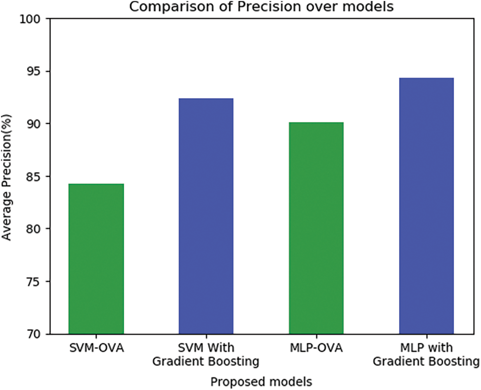
Figure 6: Precision as a performance measure for the proposed model

5  Conclusion

Cervical cancer is one of the grave diseases for many years in females. Based on the implementation of machine learning algorithms, some of the major risk factors for cervical cancer are recognized. The proposed model is implemented with the feature selection process over genetic algorithm on ensemble learning method for identifying the risk factors of cervical cancer. Depending on the feature set, the data cleaning process was done with the replacement of variables. Though these are assumptions, it is made with the help of proven techniques to fill values in the data records. It is observed that the implemented algorithms were produced significant improvement in terms of accuracy. Taken as a whole, gradient boosting algorithm with MLP classifiers produced noble outcomes with determining accuracy for the clinical symptoms of cervical cancer. This work proves that the method of using multi-layer perceptron with gradient boosting ensemble method on multi-class classification model with one vs. all show better performance measure for the identified risk factors of cervical cancer. This identified risk factors of cervical cancer from the various diagnostic methods as targets helps to understand the important causes of cervical cancer.

Funding Statement: The authors received no specific funding for this study.

Conflicts of Interest: The authors declare that they have no conflicts of interest to report regarding the present study.

References

 1.  D. S. Latha, P. Lakshmi and S. Fathima, “Staging prediction in cervical cancer patients—A machine learning approach,” International Journal of Innovative Research and Practices, vol. 2, no. 2, pp. 14–23, 2014. [Google Scholar]

 2.  K. Fernandes, D. Chicco, J. S. Cardoso and J. Fernandes, “Supervised deep learning embeddings for the prediction of cervical cancer diagnosis,” PeerJ Computer Science, vol. 4, no. 8, pp. e154, 2018. [Google Scholar]

 3.  C. J. Tseng, C. J. Lu, C. C. Chang and G. D. Chen, “Application of machine learning to predict the recurrence-proneness for cervical cancer,” Neural Computing and Applications, vol. 24, no. 6, pp. 1311–1316, 2014. [Google Scholar]

 4.  C. C. Chang, S. L. Cheng, C. J. Lu and K. H. Liao, “Prediction of recurrence in patients with cervical cancer using MARS and classification,” International Journal of Machine Learning and Computing, vol. 3, no. 1, pp. 75–78, 2013. [Google Scholar]

 5.  S. H. Ho, S. H. Jee, J. E. Lee and J. S. Park, “Analysis on risk factors for cervical cancer using induction technique,” Expert Systems with Applications, vol. 27, no. 1, pp. 97–105, 2004. [Google Scholar]

 6.  S. F. Abdoh, M. Abo Rizka and F. A. Maghraby, “Cervical cancer diagnosis using random forest classifier with SMOTE and feature reduction techniques,” IEEE Access, vol. 6, pp. 59475–59485, 2018. [Google Scholar]

 7.  T. M. Alam, M. M. A. Khan, M. A. Iqbal, W. Abdul and M. Mushtaq, “Cervical cancer prediction through different screening methods using data mining,” International Journal of Advanced Computer Science and Applications, vol. 10, no. 2, pp. 8–12, 2019. [Google Scholar]

 8.  G. Sun, S. Li, Y. Cao and F. Lang, “Cervical cancer diagnosis based on random forest,” International Journal of Performability Engineering, vol. 13, no. 4, pp. 446–457, 2017. [Google Scholar]

 9.  A. Gowda, “Feature subset selection problem using wrapper approach in supervised learning,” International Journal of Computer Applications, vol. 7, no. 1, pp. 13–17, 2010. [Google Scholar]

10. W. Yang, X. Gou, T. Xu, X. Yi and M. Jiang, “Cervical cancer risk prediction model and analysis of risk factors based on machine learning,” in Proc. of the 2019 11th Int. Conf. on Bioinformatics and Biomedical Technology, New York, pp. 50–54, 2019. [Google Scholar]

11. UCI Machine Learning Repository, “Cervical cancer (risk factors) data set,” https://archive.ics.uci.edu/ml/datasets/Cervical+cancer+%28Risk+Factors%29. [Google Scholar]

12. A. Choudhary, “Classification of cervical cancer dataset,” in Proc. of the 2018 IISE Annual Conf., Orlando, pp. 1456–1461, 2018. [Google Scholar]

13. W. R. Rudnick, M. Wrzesień and W. Paja, “All relevant feature selection methods and applications,” in Feature Selection for Data and Pattern Recognition. Studies in Computational Intelligence, U. Stańczyk, L. Jain (eds.Vol. 584. Berlin: Springer, 2015. [Google Scholar]

14. A. Sarwar, V. Sharma and R. Gupta, “Hybrid ensemble learning technique for screening of cervical cancer using Papanicolaou smear image analysis,” Personalized Medicine Universe, vol. 4, no. 1, pp. 54–62, 2015. [Google Scholar]

15. Y. E. Kurniawati, A. E. Permanasari and S. Fauziati, “Comparative study on data mining classification methods for cervical cancer prediction using pap smear results,” in 2016 1st Int. Conf. on Biomedical Engineering (IBIOMED), Indonesia, pp. 1–5, 2016. [Google Scholar]